CHAPTER 5

Analysis Of Key Topics—Sources,
Behavior, And Transport

The preceding overviews of national distribution and trends of pesticides in bed sediment
and aquatic biota, and of governing factors that affect their concentrations in these media, leaves
many specific questions unanswered. The next two chapters draw on information in the literature
reviewed to discuss, in detail, several important topics related to pesticides in bed sediment and
aquatic biota. Each key topic falls into one of two categories: (1) sources, behavior, and transport
(Chapter 5), or (2) environmental significance (Chapter 6).

5.1 EFFECT OF LAND USE ON PESTICIDE CONTAMINATION

The terrestrial environment has a strong influence on the water quality of adjacent
hydrologic systems. Both natural and anthropogenic characteristics of the terrestrial environment
are important. For example, concentrations of major chemical constituents (such as sulfate,
calcium, and pH) in a hydrologic system are influenced by geology, and the concentration of
suspended sediment is influenced by soil characteristics, topography, and land cover. Land use
activities, such as row crop agriculture, pasture, forestry, industry, and urbanization, also can
affect adjacent water bodies. Any pesticide associated with a land use can potentially find its way
to the hydrologic system and, if the pesticide has persistent and hydrophobic properties (see
Section 5.4), it will tend to accumulate in bed sediment and aquatic biota. The following section
addresses the observed link between land use and the detection of pesticides in bed sediment and
aquatic biota. Four types of land use will be discussed: agriculture, forestry, urban areas and
industry, and remote or undeveloped areas. In many cases, forested areas also could be described
as remote or undeveloped areas. The critical distinction here, however, is that many forested
areas have been managed with the use of pesticides whereas remote and undeveloped areas have
not.

5.1.1 AGRICULTURE

By far the largest use of most pesticides, both presently and historically, has been in
agriculture (Aspelin and others, 1992; Aspelin 1994). The soils of many agricultural areas still
© 1999 by CRC Press LLC

contain residues of hydrophobic, persistent pesticides that were applied during the 1970s or
earlier. This was documented in 1970 for 35 states, mostly east of the Mississippi River (Crockett
and others, 1974), in 1985 in California (Mischke and others, 1985), and during 1988–1989 in
Washington (Rinella and others, 1993). In the California study (Mischke and others, 1985), only
fields with known previous DDT use were targeted. This study obtained 99 soil samples from
fields in 32 counties. Every sample analyzed contained residues of total DDT (the sum of DDT
and its transformation products). The investigators compared the concentrations of the parent
DDT with the concentrations of its transformation products (DDD and DDE) and found that the
ratio of the parent DDT to total DDT was 0.49. That is, 49 percent of the total DDT remaining in
the soils at least 13 years after use still existed as the parent compound. In the U.S.
Environmental Protections Agency’s (USEPA) National Study of Chemical Residues in Fish
(NSCRF), which measured fish contaminants at sites in different land-use categories (such as
agricultural sites, industrial and urban sites, paper mills using chlorine, other paper mills, and
Superfund sites), sites in agricultural areas had the highest mean and median concentrations of

p

,

p

′

-DDE in fish, as well as four of the top five individual fish sample concentrations.

Agricultural sites also had the second highest mean concentration of dieldrin in fish (second to
Superfund sites), as well as two of the top five individual sample concentrations. Soils containing
residues of DDT and similar recalcitrant pesticides from past agricultural use constitute a
reservoir for these pesticides today; they have been, and will continue to be, a source of these
compounds to hydrologic systems, thus leading to contamination of surface water, bed sediment,
and aquatic biota.
Those pesticides currently used in agriculture (Table 3.5) are not as persistent as the
restricted organochlorine compounds. As discussed in Section 3.3, some moderately
hydrophobic, moderately persistent pesticides have been detected in bed sediment and aquatic
biota, although at lower detection frequencies than the more persistent organochlorine
compounds. It is probable that additional pesticides with moderate water solubilities and
persistence may be found in bed sediment or aquatic biota if they are targeted in these media (see
Section 5.4), especially in high use areas. A few moderately hydrophobic, moderately persistent
compounds were analyzed in fish by the NSCRF (U.S. Environmental Protection Agency,
1992a): dicofol, lindane,

α

-HCH, and methoxychlor (organochlorine insecticides or insecticide
components); chlorpyrifos (organophosphate insecticide); and trifluralin, isopropalin, and
nitrofen (herbicides). Of these compounds, several were found in association with agricultural
areas. Agricultural sites had the highest mean and maximum concentrations of dicofol and
chlorpyrifos, and they had the highest mean concentration of trifluralin, in fish. Moreover, sites
with the highest trifluralin residues in fish were in states with the highest agricultural use of tri-
fluralin (Arkansas, Illinois, Iowa, Minnesota, Missouri, North Dakota, South Carolina, Tennes-
see, and Texas). In California’s Toxic Substance Monitoring Program, which monitored pesti-
cides in fish and invertebrates from over 200 water bodies throughout the state, the highest
concentrations of several currently used pesticides in fish during 1978–1987 were from two
intensively farmed areas (Rasmussen and Blethrow, 1990). These pesticides are the insecticides
chlorpyrifos, diazinon, endosulfan, and parathion, and the herbicide dacthal. The highest residues

of dacthal in whole fish analyzed by the Fish and Wildlife Service’s (FWS) National
Contaminant Biomonitoring Program (NCBP) also occurred in intensively farmed areas (Schmitt
and others, 1990).
© 1999 by CRC Press LLC

5.1.2 FORESTRY

A number of studies monitored one or more pesticides in forest streams or lakes after
known application. Most of these studies were at sites in the forests of the southeastern United
States (e.g., Yule and Tomlin, 1970; Neary and others, 1983; Bush and others, 1986; Neary and
Michael, 1989), northwestern United States (e.g., Sears and Meehan, 1971; Moore and others,
1974), or Canada (e.g., Kingsbury and Kreutzweiser, 1987; Sundaram, 1987; Feng and others,
1990; Kreutzweiser and Wood, 1991; Sundaram and others, 1991). The majority of these studies
can be described as field experiments, in which a known amount of a certain pesticide was
applied to a section of a watershed, with subsequent sampling of water, bed sediment, or aquatic
biota for a period of weeks to years. These studies are considered process and matrix distribution
studies and are described in Table 2.3 (if they were conducted in United States streams and they
sampled bed sediment or aquatic biota). Few, if any, studies have reported on the ambient
concentrations of pesticides in bed sediment or aquatic biota after routine use of pesticides, so
little is known about the long-term presence of pesticides in streams from forest applications. On
the basis of the reported field experiments and information on pesticide use in forestry, a few
conclusions can be drawn.
The choice of chemicals used for forest applications has changed over time (Freed, 1984).
Before the mid-1940s, the only pesticides that were used were inorganic compounds. Organic
pesticides were introduced after World War II. Aerial spraying of pesticides began following the
availability of suitable airplanes. The chlorophenoxy acid herbicides, 2,4-D and 2,4,5-T, and the
organochlorine insecticide, DDT, were the first of the organic pesticides to be widely used. In
subsequent years, a wide variety of herbicides and insecticides were introduced into forestry use.
Most of the major classes of herbicides were represented, including triazines, ureas, uracils, and
chlorophenoxy acids. The insecticides used included most of the organochlorine compounds and

numerous organophosphate, carbamate, and pyrethroid compounds. Since the 1980s, the use of
chemical pesticides in forestry has declined (Larson and others, 1997). The chemical insecticides
have largely been replaced by biological pesticides. The current use of pesticides in forestry
(Section 3.2.2) and forestry as a source of pesticides in surface water systems (Section 4.1.1)
were previously discussed. The potential impacts on water quality are covered in more detail in
Larson and others (1997).
The pesticides used in forestry since the 1940s may have caused some environmental
impact at the time of application. However, many of these pesticides do not persist long in forest
soils or streams, so are unlikely to have lasting or long-term effects on stream biota after a period
of time (days, months, or years, depending on the chemical) has elapsed since application. The
exceptions are pesticides that are hydrophobic and recalcitrant (and thus long-lived), such as the
organochlorine insecticides. Because of their physical and chemical properties (see Section 5.4),
organochlorine insecticides may persist in bed sediment and aquatic biota of forest streams, and
forest soils containing organochlorine insecticide residues may be washed into the stream for
many years after the period of application. Also, as with pesticides applied in agricultural areas
(see Section 3.3.2), there is potential for detection of moderately hydrophobic, moderately
persistent silvicultural pesticides in bed sediment or biota, especially in high-use areas.
Triclopyr is now the highest-use herbicide on national forest land. The next most
commonly used herbicides in national forests in 1992 were 2,4-D, hexazinone, glyphosate, and
© 1999 by CRC Press LLC

picloram (Larson and others, 1997). Except for

Bacillus thuringiensis

var.

Kurstaki

(Bt), car-

baryl was the highest-use insecticide in national forests in 1992 (Larson and others, 1997). Of
these compounds, only 2,4-D was targeted in sediment or aquatic biota at more than 30 (total)
sites in all the monitoring studies reviewed (Tables 3.1 and 3.2). When data from all monitoring
studies were combined, 2,4-D was detected in 1 percent of (825 total) sediment samples and in 5
percent of (44 total) biota samples. Of the other recently used pesticides, picloram was detected
bed sediment in 2 percent of (53) samples; detection data were not reported for biota. Carbaryl
was detected in aquatic biota (11 percent of 27 samples), but not in bed sediment (only 3 samples
analyzed). Glyphosate was not detected in any of 19 total bed sediment samples; data for biota
were not reported. Triclopyr and hexazinone were not targeted in bed sediment or aquatic biota
in any of the monitoring studies reporting detection data.
Five process and matrix distribution studies (or field experiments) in forest streams provide
some indication of the behavior of organochlorine insecticides, pyrethroid insecticides, and other
selected pesticides following application in forestry. In one study in New Brunswick, Canada
(Yule and Tomlin, 1970), DDT and its transformation products, DDE and DDD, were studied in
water and bed sediment of a stream after application to nearby forests for the control of Spruce
budworm. One motivation for this study was that fish-kills occurred following the use of DDT in
forests in this area. The stream had high concentrations of DDT in the surface of the water
column immediately after application, but these subsided to the background concentration (about
0.7

µ

g/L) after a few hours. The deeper stream water (12–18 in. below the surface) did not show
the same immediate DDT concentration spike; however, DDT levels there were relatively
consistent for 2 years following the application. Twelve months after application, every bed
sediment sample (18 total) collected from the vicinity of the site of application to the mouth of
the river, about 50 mi downstream, had measurable concentrations of total DDT. The average bed
sediment concentration was about 12 percent of the forest soil concentration on a dry weight
basis. There was a trend of decreasing concentration downstream, and also a change in the ratio
of DDT/total DDT. As the distance from the point of application increased, the transformation

products constituted a greater percentage of the total DDT, indicating in-stream transformation.
Unfortunately, no time series data were presented for the bed sediment. The authors suggested
that DDT persists in forest soils, predominately as the parent compound, and that the long-term
transport to streams is through runoff of soil particles. The presence of DDT components in the
bed sediment throughout the river system 1 year after application, and the presence of DDT
components in the water 2 years after application, suggest that there is long-term storage of DDT
in the forest soil and in the bed sediment of the river system, and that the soil and bed sediment
constitute a constant source of contaminant to the river water.
Prior to its cancellation in the early 1980s, endrin was used in forestry as a coating on
aerially applied tree seeds to protect them from seed-eating rodents. One study (Moore and
others, 1974) examined the presence of this compound in the water and aquatic biota of two
Oregon watersheds after seeding. The actual amount of endrin applied to the watersheds was
estimated to be 2.5 to 10 grams a.i. per hectare. Endrin was observed consistently in the stream
water for about 9 days (maximum concentration was about 12 ng/L), then was nondetectable
until a high flow period about 21 days after application. At this time, it was detected in the water
again. This second period of detection suggests that the endrin was stored either in the forest
soils or in the bed sediment of the stream and then released with higher streamflow. Fish (coho
salmon [

Onchorhynchus kisutch

] and sculpins [family Cottidae]) and various unidentified aquatic
© 1999 by CRC Press LLC

insects were analyzed for endrin. Because of sample contamination, the results are somewhat
ambiguous. The authors did conclude that endrin was present in all biotic samples obtained
within days after application. Samples collected 12 and 30 months after the application of endrin
did not contain detectable traces of endrin. Bed sediment was not collected during this study.
A third example is the study of permethrin in Canadian streams (Kreutzweiser and Wood,
1991; Sundaram, 1991). Permethrin, a synthetic pyrethroid, is known not only for its high

insecticidal activity and its ability to control lepidopterous defoliators, but also for its high acute
toxicity to fish and strong sorption tendencies. Kreutzweiser and Wood (1991) examined the
presence of permethrin in a forest stream after aerial application. They detected the compound in
water, bed sediment, and fish. The concentration in water declined with time and distance from
application. Permethrin was seldom seen in the bed sediment of the stream (only 8 percent of the
samples). Atlantic salmon (

Salmo salar

), brook trout (

Salvelinus fontinalis

), and slimy sculpin
(

Cottus cognatus

) were analyzed, and permethrin was detected in about half of the samples
during the first 28 days after application. The fish were sampled again 69 to 73 days after
application and no traces of permethrin were detected. Sundaram (1991) studied the behavior of
permethrin by adding it directly into a forest stream. He found that it was not detected in the
stream water near the site of application after 5 hours and that it was seldom detected in the bed
sediment of the system, probably because of the low sediment organic carbon content. Sundaram
(1991) did detect permethrin in aquatic plants (water arum,

Calla palustris

), stream detritus,
caged crayfish (


Orconectes propinquus

), and caged brook trout collected during the study (up to
7 to 14 hours after application). No permethrin was detectable in caged stoneflies (

Acroneuria
abnormis

) throughout the study duration (14 hours). Permethrin also was detected in invertebrate
drift collected 280–1,700 m downstream of the application point. The longer-term presence of
permethrin in this system was not studied.
In a fourth example, 2,4-D was sprayed on clearcut forested lands in Alaska (Sears and
Meehan, 1971). The results of this study show potential for at least initial accumulation in biota.
Residues of 2,4-D were detected in river water samples (up to 200

µ

g/L), and in a single
composite sample of coho salmon fry (500

µ

g/kg), collected 3 days after spraying.
Unfortunately, later samples were not taken, so no information is provided on dissipation rates.
Finally, a dissipation study of the organophosphate pesticide chlorpyrifos-methyl was
conducted in a forest stream in New Brunswick, Canada (Szeto and Sundarum, 1981). The
results of this study indicate that there is potential for initial accumulation in stream bed
sediment and aquatic biota, but that residues are unlikely to persist. After aerial application,
chlorpyrifos-methyl residues persisted in balsam fir foliage and forest litter for the duration of

the experiment (125 days). Residues in bed sediment (10–180

µ

g/kg dry weight) persisted for at
least 10 days; at the next sampling time (105 days post-application), residues in sediment were
nondetectable (less than 1

µ

g/kg wet weight). In stream water, chlorpyrifos-methyl dissipated
rapidly within the first 24 hours after application, and it was not detectable in water (less than
0.02

µ

g/L) after four days. Residues of up to 46

µ

g/kg chlorpyrifos-methyl were detected in fish
(slimy sculpin and brook trout); only trace levels (less than 3

µ

g/kg wet weight) were detected
after 9 days, and chlorpyrifos-methyl was nondetectable (less than 1.5

µ


g/kg wet weight) after 47
days. Concentrations in brook trout were consistently higher than in slimy sculpin sampled at the
same time.
The results from these limited studies suggest that the behavior of pesticides in forested
streams are in agreement with their behavior in agricultural streams. DDT and its transformation
© 1999 by CRC Press LLC

products appear to have the longest residual time in the bed sediment. Endrin, permethrin, and
chlorpyrifos-methyl, although persisting for days to months in the bed sediment or biota,
gradually dissipated. Carbaryl, 2,4-D, and picloram are moderate in water solubility, but would
be expected to degrade in the environment eventually. Moderately hydrophobic, moderately
persistent pesticides may be expected to be found in some bed sediment or biota samples,
especially in areas of high or repeated use.

5.1.3 URBAN AREAS AND INDUSTRY

Another source of pesticides to surface water systems, and thus to bed sediment and
aquatic biota, is from urban areas. Pesticides are applied to control pests for public health or
aesthetic reasons in and around homes, yards, gardens, public parks, urban forests, golf courses,
and public and commercial buildings (Buhler and others, 1973; Racke, 1993). The available data
suggest that the patterns of urban pesticide use have changed during the past few decades, much
as has pesticide use in agriculture and forestry. Many of the high use organochlorine insecticides
have been banned and replaced by organophosphate, carbamate, and pyrethroid insecticides. The
use of herbicides in and around homes and gardens has increased, whereas herbicide applications
to industry, commercial, and government buildings and land have decreased (Aspelin, 1997).
The major pesticides used in and around homes and gardens in 1990 are listed in Table 3.5.
An examination of Table 3.5 shows that most of the organochlorine pesticides that are commonly
observed in bed sediment (Figure 3.1) and aquatic biota (Figure 3.2) are no longer used in urban
areas, with the exception of dicofol, chlordane, heptachlor, lindane, and methoxychlor. The
commercial use of existing stocks of chlordane in urban environments was banned in 1988, and

homeowner use of existing stocks is likely to have declined since then also. Although the kind of
data in Table 3.5 does not exist for the time period of the 1950s through mid-1970s, it is known
that many of the organochlorine insecticides had significant urban uses, including aldrin,
chlordane, DDT, dieldrin, endosulfan, heptachlor, and lindane (Meister Publishing Company,
1970). In 1970, lindane was used predominantly in the urban environment; there was also
considerable urban use of chlordane (Meister Publishing Company, 1970). It seems that endrin
was the exception, with little or no urban use. Of the moderately hydrophobic, moderately
persistent pesticides that have been observed, when targeted, in sediment or aquatic biota, several
are used in and around the home and garden (Table 3.5). These include chlorpyrifos, diazinon,
carbaryl, permethrin, and 2,4-D.
A number of local-scale studies have monitored pesticides in the sediment or aquatic biota
of urban areas. Mattraw (1975) examined the occurrence and distribution of dieldrin and DDT
components in the bed sediment of southern Florida. The study area included the urbanized areas
on the Atlantic coast (such as Miami and Fort Lauderdale), the Everglades water conservation
area and two nearby agricultural areas. Mattraw reported the data as concentration frequency
plots, shown in Figures 5.1 and 5.2. In the case of DDD (Figure 5.1), urban areas had a mean
concentration and a general distribution between those of the two agricultural areas, and well
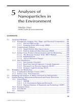
above those of the undeveloped area. In the case of dieldrin (Figure 5.2), the urban areas had a
mean bed sediment concentration and a general concentration distribution greater than all other
land use activities. In another example, Kauss (1983) measured 15 different organochlorine
insecticides and transformation products in the Niagara River below Buffalo, New York. This is
an area with many large chemical production facilities. It is thought that some of the chemicals
© 1999 by CRC Press LLC

in the sediment of this river are due either to transport from Lake Erie (the source of water for
the Niagara River) or to localized inputs. One example of a potential localized input is disposal
of 1,700 metric tons of endosulfan at disposal sites in the area. In another urban area study,
Thompson (1984) reported DDE, DDE, DDT, dieldrin, heptachlor, methoxychlor, silvex, and
2,4-D in the sediment of the Jordan River in Salt Lake City, Utah. Pariso and others (1984)
reported that DDT and chlordane were observed in bed sediment and in various species of fish

collected from the Milwaukee Harbor and Green Bay urban areas of Wisconsin, during a study
of contaminants in the rivers draining into Lake Michigan. Lau and others (1989) reported the
presence of

trans

-chlordane, DDE, DDD, and DDT in the suspended sediment of the St. Clair
and Detroit rivers on the Michigan and Ontario border. Fuhrer (1989) reported the presence of
chlordane, DDD, DDE, DDT, and dieldrin in the bed sediment of the Portland, Oregon harbor.
Capel and Eisenreich (1990) reported concentrations of

α

-HCH, DDE, DDD, and DDT in the
bed sediment and tissues of mayfly (

Hexagenia

) larvae from the harbor in Lake Superior at
Duluth, Minnesota. Crane and Younghaus-Hans (1992) detected oxadiazon residues in fish (red
shiner,

Cyprinella lutrensis

) and bed sediment from San Diego Creek, California. Oxadiazon was
also detected in transplanted clams (

Corbicula fluminea

) in the San Diego Creek and in

transplanted mussels (

Mytilis californianus

) in the receiving estuary, Newport Bay. Oxadiazon is
widely used in landscape and rights-of-way maintenance in California, and the high residues
observed in this study were attributed to its use on golf courses upstream of the study area.
Although there have been numerous local-scale studies, there has been no systematic large-
scale study of pesticides in the bed sediment or aquatic biota of urban freshwater hydrologic
systems. The National Oceanic and Atmospheric Administration’s (NOAA) National Status and
Trends (NS&T) Program targeted coastal and estuarine sites near urban population centers, and
found a correlation between most organic contaminants in bottom sediment and human
population levels (National Oceanic and Atmospheric Administration, 1991). However, there is
no comparable nationwide study of pesticides in bed sediment or aquatic biota from rivers in
urban areas. In the U.S. Geological Survey (USGS)–USEPA’s Pesticide Monitoring Network
(PMN), which sampled bed sediment from major United States rivers, only 10 of about 180 sites
sampled between 1975–1980 were in urban areas (Gilliom and others, 1985). Nonetheless, two
of these urban sites (Philadelphia, Pennsylvania, and Trenton, New Jersey) were among the 10
sites with the highest frequency of pesticide detection. The only national-scale study of
pesticides in rivers near urban centers was the USEPA’s Nationwide Urban Runoff Program
(NURP), which analyzed water samples for pesticides in urban areas nationwide during 1980–
1983 (Cole and others, 1983, 1984). The NURP samples were analyzed for the priority
pollutants, which include 20 organochlorine insecticides or transformation products, at 61
residential and commercial sites across the United States. Of these 20 organochlorine
insecticides, 13 were observed in at least one water sample. The most frequently observed
organochlorine insecticides were

α

-HCH (in 20 percent of samples), endosulfan I (in 19

percent), pentachlorophenol (in 19 percent), chlordane (in 17 percent), and lindane (in 15
percent). During this time period, all of these chemicals were still in active use in urban areas.
Because of the hydrophobicity of these compounds, their detection in the water column suggests
that they also would have been present at detectable levels in bed sediment and aquatic biota in
these urban environments.
Although many monitoring studies have reported the frequent detection of organochlorine
pesticides in bed sediment, aquatic biota, and water in urban areas, the actual sources of these
© 1999 by CRC Press LLC

pesticide residues are not completely known. Since the organochlorine insecticides had both
extensive urban and agricultural uses, their presence in urban areas could have been derived from
either source, since many urban areas are located downstream from agricultural areas.
Conversely, some rivers flowing through agricultural areas may be located downstream of urban
areas. Examples are the Mississippi River below Minneapolis and St. Paul, Minnesota, and
below St. Louis, Missouri. In such cases, residues may derive from urban, as well as from
agricultural, origin. It is reasonable to suppose that most pesticides currently in bed sediment and
aquatic biota in urban areas are derived from both agricultural and urban uses, although the
relative contribution of each of the two sources probably varies by location and compound.

1,000
100
10
1.0
0.1
0.01
0 102030405060 708090
100
Samples that equal or are less than the value indicated, in percent
DDD concentration, in ␮g/kg
Agricultural area near Everglades

Urban area
Everglades area
Eastern agricultural area
Undeveloped Big Cypress watershed

Figure 5.1.

Concentration frequency plot for DDD in bed sediment from agricultural, urban, and
undeveloped areas in southern Florida (1968–1972). Redrawn from Mattraw (1975) with permission of the
author.
© 1999 by CRC Press LLC

5.1.4 REMOTE OR UNDEVELOPED AREAS

Pesticides, particularly the organochlorine insecticides, are often observed in bed sediment
and aquatic biota in remote areas of the United States and of the rest of the world. Their presence
in remote or undeveloped areas is seldom due to local use, but rather to atmospheric transport
and deposition. Majewski and Capel (1995) have reviewed the presence and movement of pesti-
cides in the atmosphere and the deposition processes involved in their delivery to remote areas.
For some pesticides, particularly the organochlorine insecticides, regional atmospheric transport
is common and serves as a mechanism to disperse them throughout the world, particularly
toward the polar regions.

Agricultural area near Everglades
Urban area
Everglades area
Eastern agricultural area
Undeveloped Big Cypress watershed
1,000
100

10
1.0
0.1
0.01
10 20 30 40 50 60 70 80 90 1000
Sample that equal or are less than value indicated, in percent
Dieldrin concentration, in ␮g/kg

Figure 5.2.

Concentration frequency plot for dieldrin in bed sediment from agricultural, urban, and
undeveloped areas in southern Florida (1968–1972). Redrawn from Mattraw (1975) with permission of the
author.
© 1999 by CRC Press LLC

Pesticides are introduced into the atmosphere either by volatilization or wind erosion. Once
they are in the atmosphere, they can either be deposited locally (in the range of tens of kilo-
meters) or move into the upper troposphere and stratosphere for more widespread regional, or
possibly global, distribution. Once in the upper atmosphere, the global wind circulation patterns
control their long-range transport. The general global longitudinal circulation is a form of ther-
mal convection driven by the difference in solar heating between equatorial and polar regions.
Over the long-term, upper air masses tend to be carried poleward and descend into the subtrop-
ics, subpolar, or polar regions. These air masses are then carried back toward the tropics in the
lower atmosphere (Levy, 1990). Once in the atmosphere, the residence time of a pesticide
depends on how efficiently it is removed by either deposition or chemical transformation. Atmos-
pheric deposition processes can be classified into two categories: those involving precipitation
(wet deposition) and those not involving precipitation (dry deposition). The effectiveness of a
particular removal process depends on the physical and chemical properties of the pesticide, the
meteorological conditions, and the terrestrial or aquatic surface to which deposition is occurring.
Risebrough (1990) described the airborne movement of pesticides from their point of applica-

tion as a global gas-chromatographic system where pesticide molecules move many times
between the vapor-soil-water-vegetation phases, maintaining an equilibrium of chemical poten-
tial between these phases. That is, after a pesticide is deposited from the atmosphere to a terres-
trial or aquatic surface, it can reenter the atmosphere and be transported and redeposited down-
wind repeatedly until it is chemically transformed or globally distributed.
Virtually all studies of pesticides in remote areas have been conducted on remote lakes and
oceans, rather than on rivers and streams. A few examples of these studies will be presented to
illustrate the global nature of atmospheric deposition. One of the earliest reports that attributed
the presence of DDT in a remote surface water body to atmospheric deposition was a study by
Swain (1978) conducted in the national park in Isle Royale, Michigan. Although this island is in
Lake Superior and is removed hundreds of kilometers from agricultural uses of DDT, DDT was
found in the water, sediment, and fish (lake trout,

Salvelinus namaycush

, and lake whitefish,

Coregonus clupeaformis

) of Siskitwit Lake on Isle Royale. The probable explanation for this
contamination was through atmospheric deposition. Organochlorine contamination of air, snow,
water, and aquatic biota in the Arctic has been extensively studied (Hargrave and others, 1988;
Patton and others, 1989; Bidleman and others, 1990; Gregor, 1990; Muir and others, 1990) and
also is attributed to atmospheric transport. All of the common organochlorine insecticides have
been observed in Arctic studies, but the two most prevalent were

α

-HCH and lindane. These are
the two organochlorine insecticides with the highest vapor pressures and their abundance sup-

ports the idea of the global gas-chromatographic effect of pesticides being transported to the
polar regions described above. Although organochlorine concentrations in the Arctic water are
low, these contaminants bioaccumulate in aquatic biota and appear to be magnified in aquatic
and terrestrial food webs, reaching quite elevated levels in the Arctic mammals. Addison and
Zinck (1986) found that the DDT concentration in the Arctic ringed seal (

Phoca hispida

) did not
decrease significantly between 1969 and 1981, while the concentration of polychlorinated biphe-
nyls (PCB) did decline. They attributed this to continued atmospheric deposition of DDT from
its use in areas of eastern Europe during this time, compared with declining global PCB use.
© 1999 by CRC Press LLC

5.2 PESTICIDE UPTAKE AND ACCUMULATION BY AQUATIC BIOTA

Historically, there has been controversy in the literature as to the mechanisms of contami-
nant uptake and bioaccumulation by aquatic biota. Probably the strongest controversy concerns
whether biomagnification occurs in aquatic systems. In common usage, “biomagnification” may
refer either to a process or to an effect (or phenomenon). The biomagnification process, in which
the tissue concentrations of a contaminant increase as it passes up the food chain through two or
more trophic levels, results in the phenomenon of biomagnification, in which organisms at
higher trophic levels are observed to possess higher contaminant levels than their prey. An alter-
native school of thought holds that contaminant accumulation by aquatic organisms can be
described using equilibrium partitioning theory, in which contaminant concentrations in water,
blood, and tissue lipids approach equilibrium and the concentrations in these phases are related
by partition coefficients. Regardless of the mechanism of uptake, the contaminant partitions into
and out of these phases according to its relative solubility. Until fairly recently, biomagnification
and equilibrium partitioning theories were considered mutually exclusive, since the phenome-
non of biomagnification appeared to violate thermodynamic conditions of equilibrium. However,

recent equilibrium partitioning models have attempted to incorporate and explain the biomagnifi-
cation process (see Section 5.2.5).
The relative importance of contaminant uptake from the diet and from water via
partitioning has also been debated in the literature. Although dietary uptake has been associated
with biomagnification and uptake by partitioning with equilibrium partitioning theory, this is not
a true dichotomy. Uptake of a contaminant by aquatic organisms can occur via partitioning of the
contaminant from water, pore water, or sediment; and via ingestion of contaminated food or
sediment. These are not mutually exclusive mechanisms of uptake, and indeed it is frequently
assumed that bioaccumulation in the field results from multiple routes of uptake. Dietary uptake
is not inconsistent with equilibrium partitioning theory; the critical issue in equilibrium
partitioning theory is that, however a contaminant enters an organism, it will partition within the
organism or be eliminated from the organism according to its relative solubility in these
compartments, or phases.
Hundreds of laboratory and field studies have been performed that attempt to elucidate
uptake mechanisms or to test the theories of biomagnification or equilibrium partitioning.
Although each theory has been the dominant one at some time in the past, the extensive discus-
sion and effort put into experimentation, field monitoring, and modeling during the past three
decades have begun to achieve some resolution between the two schools of thought. In sum-
mary, the route of uptake (diet versus partitioning) and the mechanism of bioaccumulation
(biomagnification versus equilibrium partitioning) in aquatic systems appear to depend on the
characteristics of the chemical (such as hydrophobicity, and molecular weight and structure), on
the organisms involved (such as species, age, body size, reproductive state, lipid content, and
metabolic capability), and on environmental factors (such as temperature).
In the remainder of this section, some terminology and simple models of bioaccumulation
are defined (Section 5.2.1). Next, the two theories of biomagnification (Section 5.2.2) and equi-
librium partitioning (Section 5.2.3) are described, and then some laboratory and field studies that
© 1999 by CRC Press LLC

attempted to test these theories are examined (Section 5.2.4). Finally, an emerging resolution
between competing mechanisms of bioaccumulation is presented by describing the current

understanding of the processes of uptake and elimination; the biological, chemical, and environ-
mental factors that affect contaminant accumulation; and examples of some different types of
bioaccumulation models (Section 5.2.5).

5.2.1 BIOACCUMULATION TERMINOLOGY AND SIMPLE MODELS

In the early literature, individual authors defined their own terminology to describe uptake
and accumulation by biota. Because the same terms were not used consistently by different
authors, this added confusion to the already complex subject under investigation. Today,
conventional definitions of several terms exist that have facilitated organized discussion of
contaminant uptake mechanisms. These terms were introduced in Section 4.3, and are described
in more detail below. In general, contaminant accumulation can be viewed as a function of
competing processes of uptake and elimination.

Bioconcentration

refers to chemical residue obtained directly from water via gill or
epithelial tissue (Brungs and Mount, 1978). The bioconcentration process is viewed as a balance
between two kinetic processes, uptake and elimination, as quantified by pseudo-first-order rate
constants

k

1

and

k

2


, respectively.

dC

b

/

dt

=

k

1

C

w

−

k

2

C

b


(5.1)
where

C

b

is the concentration in biota (in units of pesticide mass per tissue mass) and

C

w



is the
concentration in the surrounding water (in units of pesticide mass per volume). The elimination
constant,

k

2

, refers to diffusive release only. This simple model assumes that there is no
contaminant uptake from food, no metabolism, no excretion, and no growth dilution. The

bioconcentration factor

(BCF) is defined as the ratio of a contaminant concentration in biota to

its concentration in the surrounding medium (water). At long exposure times (equilibrium), the
BCF also equals the ratio of the uptake constant (

k

1

) to the elimination constant (

k

2

) (Mackay,
1982).
BCF =

C

b

/

C

w

=

k


1

/

k

2

(5.2)
The BCF can be measured in the laboratory in either of two ways. First, using the steady-
state approach, biota (usually fish) are exposed to an aqueous solution of the target contaminant
for a fixed length of time. The BCF then is calculated as the ratio of the concentration measured
in fish to the concentration measured in water at the end of the experiment. Second, using the
kinetic approach, uptake and elimination rate constants are measured in separate experiments and
the BCF is calculated as the ratio

k

1

/

k



2

. At equilibrium, the two methods should give the same

results. For extremely hydrophobic contaminants that require a long time to reach equilibrium,
the kinetic approach permits estimation of the BCF over a shorter exposure time.

Bioaccumulation

is the process whereby a chemical enters an aquatic organism through the
gills, epithelial tissue, dietary intake, and other sources (Brungs and Mount, 1978). Use of this
© 1999 by CRC Press LLC

term does not imply any particular route of exposure. It is commonly used when referring to
field measurements of contaminant residues in biota, where the routes of exposure are unknown.
Bioaccumulation, like bioconcentration, is viewed as a balance between processes of uptake and
elimination, except that in a bioaccumulation model, multiple routes of uptake and elimination
are possible. The kinetics of a bioaccumulation model can be described as:

(5.3)

This specific model considers uptake via water and food, as well as elimination via
excretion from gills and feces, biotransformation, reproduction, and growth (Gobas and others,
1989b; Sijm and others, 1992). The terms are defined as follows:

C

b

is the concentration in biota;

C

w




is the concentration in water;

C

f

is the concentration in food;

k

1

and

k

2

are diffusion-
controlled constants for uptake and elimination, respectively;

α

is the absorption efficiency of a
chemical from food, which varies from 0 to 1;

β


is the food consumption rate;

k

e

is the rate
constant for elimination in feces;

k

m

is the biotransformation rate constant;

k

r

is the zero-order
reproduction rate;

R

is a trigger value that is either 0 or 1 (depending on whether reproduction
takes place or not); and

G


is the growth dilution factor. The

bioaccumulation factor

(BAF) is
analogous to the BCF, but applies to field measurements or to laboratory measurements with
multiple exposure routes. The BAF is the ratio of contaminant concentration measured in biota
in the field (or under multiple exposure conditions) to the concentration measured in the
surrounding water. At steady state, chemical fluxes into and out of the fish are equal, so the
quantity (

dC

b

/

dt

) equals zero. Therefore:

(5.4)

where BCF

f

is the bioconcentration factor of the food (i.e., the ratio of

C


f

/

C

w

).

Biomagnification

is the process whereby the tissue concentrations of a chemical increase as
it passes up the food chain through two or more trophic levels (Brungs and Mount, 1978).
Biomagnification is also called the “food chain effect.” Occasionally, the term

biomagnification
factor

(BMF) is used in the literature to refer to the ratio of contaminant concentration in biota to
that in the surrounding water when the biota was exposed via contaminated food.

5.2.2 BIOMAGNIFICATION

In theory, biomagnification begins with ingestion by a predator of a lower trophic level
organism whose tissues contain contaminant residues. This theory was supported initially by
field observations and later by food chain models (see Section 5.2.4). These include many
observations of increasing contaminant residues at higher trophic levels, as well as higher
residues of metabolites in predators than prey. Also, field-measured BAFs often were higher than

BCFs measured in the laboratory during water-only exposures, indicating that partitioning from
water did not adequately account for residues bioaccumulated by aquatic organisms in natural
systems.
The available evidence suggests that biomagnification may occur under conditions of low
water concentration for compounds of high lipophilicity, high persistence, and low water
dC
b
dt⁄ k
1
C
w
αβC
f
k
2
C
b
k
e
C
b
k
m
C
b
Rk––
r
C
b
GC

b
–––+=
BAF C
b
C
w
⁄ k
1
αβBCF
f
+()k
2
k
e
k
m
Rk
r
G++ + +()⁄==
© 1999 by CRC Press LLC

solubility (Biddinger and Gloss, 1984). Biomagnification is most likely to occur for chemicals
with log

n

-octanol-water-partition coefficient (

K


ow
) values greater than 5 or 6 (Connell, 1988;
Gobas and others, 1993b) and for top predators with long lifetimes. Dietary intake and
biomagnification are very important for air-breathing vertebrates (see Section 5.2.5, subsection
on Uptake Processes).
The mechanism by which biomagnification operates is not completely understood. As
previously noted, this subject has been controversial, since biomagnification appeared to be
inconsistent with thermodynamic conditions (see Section 5.2.5, subsection on Dietary Uptake
and Biomagnification). During the 1960s, the hypothesis prevailed that bioaccumulation in
aquatic systems was controlled by mass transfer through the food chain (Rudd, 1964; Hunt,
1966; Woodwell, 1967; Woodwell and others, 1967; Harrison and others, 1970). This was based
on the observation that hydrophobic chemical concentrations increased with increasing trophic
levels in aquatic systems (Hunt and Bischoff, 1960; Woodwell, 1967; Woodwell and others,
1967) and by analogy to terrestrial species, for which food was usually the dominant route of
uptake (Moriarty and Walker, 1987). This food chain effect was traditionally explained by the
loss of biomass in the food chain due to respiration and excretion as biomass is transferred from
one trophic level to the next (Woodwell, 1967). This assumes that, for each step in the food
chain, more chemical residues are retained than energy or body mass (Hamelink and Spacie,
1977).
Subsequently, it was pointed out (Hamelink and Spacie, 1977) that this mechanism must
take growth efficiency and dietary uptake efficiency into account. The growth efficiency of fish is
about 8 percent: thus dietary uptake efficiencies should exceed this value for any increase in
contamination to occur (Connell, 1988). Dietary uptake efficiencies reported for some
organochlorine compounds in fish ranged from 9 to 68 percent and tend to decline with
increasing concentration, reaching a steady state (Hamelink and Spacie, 1977). Moreover, some
observations of food chain effects can be explained by lipid-based partitioning (Section 5.2.3,
Relation Between Contaminant Residues and Trophic Levels). The original mass-transfer
mechanism is now considered unlikely to account for steadily increasing contaminant
concentration with increasing trophic level (Connell, 1988). More recently, it was proposed that
food digestion and absorption from the gastrointestinal tract, accompanied by inflow of more

contaminated food, increase the concentration of the chemical in the gastrointestinal tract relative
to that in the original food (Connolly and Pedersen, 1988; Gobas and others, 1988, 1993b; also
see Section 5.2.5, subsection on Uptake Processes).
5.2.3 EQUILIBRIUM PARTITIONING THEORY
The hypothesis of food chain transfer was first questioned around 1971 (Hamelink and
others, 1971; Woodwell and others, 1971). Hamelink and others (1971) instead proposed that
organisms continuously exchange pesticide residues with the surrounding water, in theory
reaching a chemical equilibrium with their environment. As an approximation, the organism was
viewed as a pool of lipophilic material, and contaminant accumulation was proposed to be
controlled by sorption to body surfaces and partitioning into lipids from water. This equilibrium
partitioning hypothesis prevailed for almost 15 years (e.g., National Research Council, 1979,
1985; Levin and others, 1985). Recently, some equilibrium partitioning models have attempted
to incorporate dietary intake and to explain the phenomenon of biomagnification (Section 5.2.5).
© 1999 by CRC Press LLC
The equilibrium partitioning theory holds that, at equilibrium, the thermodynamic activity
of a chemical will be the same in all phases of the system (Hamelink and others, 1971). The
organism is considered to be a single, uniform compartment, with the solubility of the chemical
in the organism controlled by the chemical's solubility in lipid. The rate of uptake is controlled
by the concentration gradient between the organism and the surrounding water. This simple
model assumes the following: uptake and elimination show pseudo-first-order kinetics; uptake is
limited only by diffusion; the BCF is controlled by the hydrophobicity of the chemical and the
lipid content of the fish; and there is negligible growth or metabolism. This theory was supported
by laboratory experiments that demonstrated that experimentally determined values for BCF
were directly correlated with the K
ow
, and inversely correlated with water solubility (Section
5.2.4). n-Octanol is a convenient surrogate for the lipid phase (Mackay, 1982), and the K
ow
is a
useful estimate of the degree of hydrophobicity (Farrington, 1989). Laboratory experiments that

show correlations between BCF and chemical properties do not prove the equilibrium
partitioning theory, but they are consistent with it. On the other hand, instances where BCF fails
to correlate with these chemical properties may indicate limitations in the equilibrium
partitioning model.
One key bioaccumulation model (also see Section 5.2.5, subsection on Bioaccumulation
Models) is the fugacity model developed by Mackay (1982). This is a simple equilibrium
partitioning model that views an organism as an inanimate volume consisting of multiple phases
of differing chemical composition. A chemical diffuses between the organism and water because
of a concentration gradient. The rate of uptake can be expressed using Fick's law, which holds
that sorption of a lipid-soluble chemical through an integument is generally pseudo-first-order,
with the rate of sorption proportional to the surface area and concentration of the diffusing
chemical, and inversely proportional to the thickness of the integument. When the two phases
(organism and water) are not in equilibrium, the concentration gradient determines which
direction the chemical will diffuse to reach equilibrium. This situation can be described using
fugacity concepts and terminology. In general, fugacity is a thermodynamic measure of the
escaping tendency of a chemical from a phase, and is equivalent to chemical activity or potential.
Fugacity has units of pressure and is proportional to concentration in the phase. Mass diffuses
from high to low fugacity under nonsteady-state conditions. When the escaping tendencies of a
chemical from two phases are equal, the phases are in equilibrium. According to the fugacity
model, contaminant uptake by the organism is determined by the chemical fugacity differential
between the organism and the surrounding medium (water). At low concentrations (such as those
that commonly occur in the environment), fugacity is related to concentration as follows:
C = (Z)(f) (5.5)
where C is concentration (in units of mole per cubic meter, or mol/m
3
), f is fugacity (Pascal), and
the proportionality constant Z is the fugacity capacity (mol/m
3
/Pascal). The fugacity capacity
depends on the temperature, the pressure, the chemical, and the environmental medium; it

quantifies the capacity of each phase for fugacity. For biota, actual uptake may be a combination
of uptake from the surrounding medium (water) and from food, which also may be at or
approaching equilibrium with the surrounding water.
Some of the predictions of the fugacity model have been tested using field data (Section
5.2.4). For example, in its simplest form, the fugacity model predicts that the animal/water
© 1999 by CRC Press LLC
fugacity ratio will be 1 at equilibrium and that the concentration of a contaminant in the lipids of
all animals must be equal, regardless of trophic position. This condition is termed equifugacity.
Only under nonequilibrium conditions may the fugacity ratio deviate from 1.
5.2.4 EVIDENCE FROM LABORATORY AND FIELD STUDIES
Some key laboratory and field studies that attempted to test the validity of the
biomagnification or equilibrium partitioning theories are discussed in this section. Some studies
looked for evidence of biomagnification in the field, and other studies attempted to test pre-
dictions of equilibrium partitioning theory. These studies have helped to elucidate the biological,
environmental, and chemical factors that affect bioaccumulation.
Evidence of Biomagnification in the Field
Three types of evidence of biomagnification in the field will be discussed: (1) correlations
between contaminant concentrations and trophic levels in aquatic biota, (2) comparison of
laboratory BCFs that are based on water exposure only with field-measured BAFs, and (3)
development and validation of food chain models.
Effect of Trophic Level on Contaminant Concentrations
There are many examples of field studies in which contaminant concentrations in aquatic
biota were observed to increase with increasing trophic levels. In a Long Island (New York) salt
marsh, DDT residues in marine organisms increased with increasing organism size and
increasing trophic level (Woodwell and others, 1967). Total DDT residues ranged over three
orders of magnitude, from 40
µg/kg wet weight in plankton to 2,070 µg/kg in a carnivorous fish
(the Atlantic needlefish, Strongylura marina) to 75,500
µg/kg in ring-billed gulls (Larus
delawarensis), as shown in Table 5.1. In later examples, accumulation was found to be directly

related to position in the food chain for the following: chlordane, total DDT, and dieldrin in
zooplankton, forage fish, and predator fish in the Great Lakes (Whittle and Fitzsimons, 1983);
total DDT in amphipods (Pontoporeia affinis), various fish species, and ducks from Lake
Michigan (Ware and Roan, 1970); DDT in krill, benthic fish, and Weddell seals (Leptonychotes
weddelli) in the Antarctic Ocean (Hidaka and others, 1983); kepone in the James River food
chain (Connolly and Tonelli, 1985); PCBs in the lake trout food chain in Lake Michigan
(Thomann and Connolly, 1984); PCBs in the yellow perch (Perca flavescens) food chain in the
Ottawa River (Norstrom and others, 1976); organochlorine compounds in micro- and macro-
zooplankton off the Northumberland coast (Robinson and others, 1967); pesticides and PCBs in
periphyton, green algae, macrophytes, snails, and various fish in the Schuylkill River, Pennsyl-
vania (Barker, 1984); and hexachlorobenzene and PCBs in white bass (Morone chrysops) from
Lake Erie (Russell and others, 1995). Tanabe and others (1984) reported increasing concen-
trations from zooplankton to squid for total DDT and PCBs, but not for total HCH (which is less
hydrophobic and has a lower K
ow
). In examining field data on residues in benthic animals from
© 1999 by CRC Press LLC
Sample
DDT
Residues
(mg/kg)
Percentage of Residue as:
DDT DDE DDD
Water
11
0.00005 — — —
Plankton, mostly zooplankton 0.040 25 75 Trace
Cladophora gracilis 0.083 56 28 16
Shrimp
2

0.16 16 58 26
Opsanus tau, oyster toadfish (immature)
2
0.17 None 100 Trace
Menidia menidia, Atlantic silverside
2
0.23 17 48 35
Crickets
2
0.23 62 19 19
Nassarius obsoletus, mud snail
2
0.26 18 39 43
Gasterosteus aculeatus, threespine stickleback
2
0.26 24 51 25
Anguilla rostrata, American eel (immature)
2
0.28 29 43 28
Flying insects, mostly Diptera
2
0.30 16 44 40
Spartina patens, shoots 0.33 58 26 16
Mercenaria mercenaria, hard clam
2
0.42 71 17 12
Cyprinodon variegatus, sheepshead minnow
2
0.94 12 20 68
Anas rubripes, black duck 1.07 43 46 11

Fundulus heteroclitus, mummichog
2
1.24 58 18 24
Paralichthys dentatus, summer flounder
3
1.28 28 44 28
Esox niger, chain pickerel 1.33 34 26 40
Larus argentatus, herring gull, brain (d) 1.48 24 61 15
Strongylura marina, Atlantic needlefish 2.07 21 28 51
Spartina patens, roots 2.80 31 57 12
Sterna hirundo, common tern (a) 3.15 17 67 16
Sterna hirundo, common tern (b) 3.42 21 58 21
Butorides virescens, green heron (a) (immature, found dead) 3.51 20 57 23
Larus argentatus, herring gull (immature) (a) 3.52 18 73 9
Butorides virescens, green heron (b) 3.57 8 70 22
Larus argentatus, herring gull, brain
4
(e) 4.56 22 67 11
Sterna albifrons, least tern (a) 4.75 14 71 15
Sterna hirundo, common tern (c) 5.17 17 55 28
Table 5.1. Residues of total DDT in samples from the Carmans River Estuary, Long Island, New York
[Residues are in mg/kg wet weight of the whole organism, unless otherwise indicated. Proportions of DDD, DDE,
and DDT are expressed as a percentage of total DDT. Letters in parentheses indicate replicate samples in original
reference as follows: there were three common tern replicates (a–c), two green heron replicates (a–b), six herring
gull replicates (a–f), and 2 least tern replicates (a–b). Abbreviations and symbols: mg/kg, milligrams per kilogram;
—, no data. Reproduced from Woodwell and others (1967) with permission of the publisher. Copyright 1967
American Association for the Advancement of Science]
© 1999 by CRC Press LLC
the Great Lakes, Bierman (1990) observed that body burdens of various organic chemicals were
significantly higher for carp than for all other organisms, and higher than predicted by

equilibrium partitioning theory. However, body burdens in forage fish were not significantly
different from those in benthic macroinvertebrates.
Moreover, several authors reported that the relative concentration ratios of pesticides to
pesticide metabolites in fish varied with respect to trophic levels. Fish at higher trophic levels
contained a higher percentage of pesticide metabolites (DDE, DDD, heptachlor epoxide,
dieldrin) than fish at lower trophic levels (Hannon and others, 1970; Johnson, 1973). Organisms
at lower trophic levels had proportionally more DDT (parent compound) residues, relative to
organisms at higher trophic levels (Woodwell and others, 1967; Johnson, 1973).
In some studies, no clear relation between hydrophobic contaminant residues and trophic
level was observed. Examples include the following: dieldrin in aquatic invertebrates in the
Rocky River, South Carolina (Wallace and Brady, 1971); PCBs in cod (Gadus morhua) (livers
and fillets) and prey organisms from the western Baltic Sea (Schneider, 1982); and organo-
chlorine residues in amphipods and other stream animals from Swedish streams (Sodergren and
others, 1972). The lack in finding any food chain effects has been attributed to the complexity of
food chains in the communities sampled (Schneider, 1982), differences in metabolic capability,
habitat conditions, seasonal effects, or subtle differences in feeding strategy (Wallace and Brady,
1971).
Hamelink and others (1971) conducted mesocosm studies investigating the behavior of
DDT in food chains. Fish rapidly accumulated total DDT after p,p′-DDT was added to the water,
and there was no difference in residues between complete food chains (algae, invertebrates, fish),
Sample
DDT
Residues
(mg/kg)
Percentage of Residue as:
DDT DDE DDD
Larus argentatus, herring gull (immature) (b) 5.43 18 71 11
Larus argentatus, herring gull (immature) (c) 5.53 25 62 13
Sterna albifrons, least tern (b) 6.40 17 68 15
Sterna hirundo, common tern (five abandoned eggs) 7.13 23 50 27

Larus argentatus, herring gull (d) 7.53 19 70 11
Larus argentatus, herring gull
4
(e) 9.60 22 71 7
Pandion haliaetus, osprey (one abandoned egg)
5
13.8 15 64 21
Larus argentatus, herring gull (f) 18.5 30 56 14
Mergus serrator, red-breasted merganser (1964)
3
22.8 28 65 7
Phalacrocorax auritus, double-crested cormorant (immature) 26.4 12 75 13
Larus delawarensis, ring-billed gull (immature) 75.5 15 71 14
Table 5.1. Residues of total DDT in samples from the Carmans River Estuary, Long Island, New
York—Continued
1
In units of milligrams per liter.
2
Composite sample of more than one individual.
3
From Captree Island, New York, 20 miles (32 kilometers) west-southwest of study area.
4
Found moribund and emaciated, north shore of Long Island, New York.
5
From Gardiners Island, Long Island, New York.
© 1999 by CRC Press LLC
or broken food chains (algae, fish; or algae, invertebrates). These authors observed a stepwise
increase in residue levels between trophic levels, whether or not food chains were broken or
complete. They questioned the biomagnification theory and proposed that the uptake mechanism
involved sorption and partitioning into body lipids. One factor complicating interpretation of

these results is that the broken food chains were fed, while those in the complete food chains
were not, even though the food supply was inadequate to maintain the fish in prime condition.
Biddinger and Gloss (1984) reviewed field, laboratory, and artificial ecosystem studies that
assessed bioconcentration, dietary uptake, and potential biomagnification of organic contami-
nants. They concluded that food chain biomagnification was not well substantiated in the
literature at that time, but that it was most likely to occur under conditions of low water concen-
tration for compounds of high lipophilicity, low water solubility, and high persistence. They also
pointed out that most cases of high residues that occurred in organisms of high trophic levels had
not been shown to be the result of trophic transfer; rather, factors such as age, size, sex, season,
lipid content, and physical condition may have been involved. This does not disprove the theory
of biomagnification, but merely illustrates the difficulty in deducing cause and effect from field
studies.
The observed progression in residue levels with trophic level was explained by some
authors as an artifact that organisms at higher trophic levels have greater lipid pools than those at
lower trophic levels (Hamelink and others, 1971; Clayton and others, 1977; Goerke and others,
1979; Ellgehausen and others, 1980). This suggests that lipid normalization of residues would
reduce or eliminate any trophic level effect observed for wet-weight residues, which was the case
in a few studies. When concentrations were lipid-normalized, mean PCB concentrations for
marine zooplankton were similar to those for marine fish (such as herring and salmon—species
not specified) (Clayton and others, 1977). PCB levels per weight of extractable lipids in cod (G.
morhua) and prey organisms from the western Baltic Sea were more uniform than wet weight
residues, indicating the important role of lipids in PCB bioaccumulation (Schneider, 1982). Lipid
content and composition have been suggested as one basis for seasonal effects in contaminant
accumulation (discussed in Section 5.3.5), as well as for differences among species and tissue
types (discussed in Section 5.2.4, subsection on Lipid Normalization).
Other explanations have been offered as the basis for the trophic level effects commonly
observed in the field. Biddinger and Gloss (1984) noted that increases in contaminants with
trophic level have occurred only for a few extremely hydrophobic contaminants (such as DDT
and PCBs), and these increases generally were less than an order of magnitude over the whole
aquatic food chain. The apparent trophic level effects observed in field surveys have been attrib-

uted to nonequilibrium conditions that exist in the field; because the direct uptake (via
partitioning) of extremely hydrophobic compounds is slow, feeding may provide significant
exposure to these compounds for high trophic levels (Connolly and Pedersen, 1988). Also,
because population turnover rates are more rapid at lower and intermediate trophic levels than at
high trophic levels, it has been suggested that apparent biomagnification may be an artifact of the
period of exposure of different trophic levels (Grzenda and others, 1970).
There remain some observations of trophic level effects in the field that have not been
explained by differences in lipid content or other factors. For example, Crossland and others
(1987) monitored distribution of 2,5,4′-trichlorobiphenyl in ponds stocked with grass carp
© 1999 by CRC Press LLC
(Ctenopharyngodon idella) and rainbow trout (Oncorhynchus mykiss). By eight days after
exposure began, the trout had significantly higher residues than carp on a lipid-weight basis. The
stomach contents of the fish were examined to determine what foods were consumed. The
stomach contents of all of the grass carp contained aquatic vegetation and no invertebrates,
whereas those of all of the trout contained zooplankton, snails, arthropods, and no aquatic
vegetation. The higher accumulation of 2,5,4′-trichlorobiphenyl by trout could not be explained
in terms of differences in lipid content, growth rates, or metabolic rates. Crossland and others
(1987) suggested that accumulation via the food chain was responsible. In another example,
lipid-based BCF values did not explain the high PCB concentrations observed at upper trophic
levels in Lake Michigan (Thomann and Connolly, 1984). Also, lipid-normalized PCB residues in
four invertebrate species and one fish species (sole, Solea solea) from the Wadden Sea were
correlated with trophic level (Goerke and others, 1979).
Bioaccumulation Factors
For extremely hydrophobic contaminants, BAF values measured in field surveys (where
biota may be exposed to contaminants via multiple routes, such as water, food, and sediment) are
commonly higher than BCF measurements made in the laboratory on the basis of aqueous
exposure only. For example, this has been observed for DDT (Biddinger and Gloss, 1984),
hexachlorobenzene (Oliver and Niimi, 1983), mirex (Oliver and Niimi, 1985), and PCBs (Oliver
and Niimi, 1985; Porte and Albaiges, 1994). Some authors have concluded that uptake from
water alone underestimates residues of these contaminants in aquatic biota, indicating that these

residues are partly derived from dietary uptake (Biddinger and Gloss, 1984; Oliver and Niimi,
1985; Porte and Albaiges, 1994). In contrast, for hydrophobic contaminants with short half-lives
in fish, laboratory-derived BCFs were comparable with field-measured BAFs. Examples include
lindane,
α-HCH, 1,2,4-trichlorobenzene, and 1,2,3,4-tetrachlorobenzene in rainbow trout from
Lake Ontario (Oliver and Niimi, 1983, 1985). For these compounds, direct uptake from water
can account for residues observed in field surveys.
The observation that field-based BAF measurements are higher than laboratory-derived
BCF values for some contaminants does not by itself indicate food chain transfer. Because
organisms in the field are exposed over a lifetime, they may be closer to equilibrium than in
short-term laboratory experiments (Connolly and Pedersen, 1988). This is particularly relevant
for extremely hydrophobic compounds, since the time to achieve equilibrium increases with
increasing K
ow
(Veith and others, 1979a; Hawker and Connell, 1985). This is illustrated in
Figure 5.3 for chlorobenzenes in rainbow trout (Oliver and Niimi, 1983). The higher the degree
of chlorination, the longer it was required for the systems to equilibrate, and thus, the higher the
BCF value. Hexachlorobenzene did not reach equilibrium within the duration of the experiments
(about 120 days). Oliver and Niimi (1985) subsequently reported that p,p′-DDE, cis- and trans-
chlordane, several PCB congeners (18, 40, 52, 101, 155), octachlorostyrene, and mirex did not
reach equilibrium in 96-day laboratory experiments to measure BCF values.
For contaminants that take a long time to reach equilibrium, the field-based BAF can be
compared with the BCF at theoretical equilibrium, which is estimated using the kinetic approach.
As described in Section 5.2.1, this entails measuring the uptake and elimination rate constants in
separate experiments, then calculating the BCF as the ratio of the rate constants (Equation 5.2).
In contrast, the BCF that is measured using the steady-state approach (in which the BCF is
© 1999 by CRC Press LLC
PeCB
HCB
1,2,4,5-TeCB

1,2,3,4-TeCB
1,3,5-TCB
1,2,4-TCB
1,2,3-TCB
1,3-DCB
1,4-DCB
1,2-DCB
4
3
2
0
20 40 60 80 100 120
Exposure time, in days
Log BCF
calculated as the ratio of the measured concentrations of the contaminant in fish and in water at
the end of the exposure time) is likely to underestimate the BCF value for compounds that
require a long time to reach equilibrium. In tests with rainbow trout, kinetic and steady-state
BCF values were similar for compounds (such as lindane) with short half-lives in fish (less than
about 30 days). For compounds with longer half-lives in fish, the two BCF values did not agree;
the steady-state approach underestimated the BCF because steady state probably had not yet
been reached for chemicals that were eliminated slowly by fish (Oliver and Niimi, 1985). These
laboratory-derived BCFs were compared with field BAFs for rainbow trout from Lake Ontario
(Oliver and Niimi, 1985). Predicted BAF values (based on laboratory BCFs) for lindane,
α-HCH,
1,2,4-trichlorobenzene, and 1,2,3,4-tetrachlorobenzene were close to the observed BAF values.
These compounds all have short half-lives in fish. For compounds (such as PCBs) with longer
half-lives in fish, both steady-state and kinetic BCFs underestimated field BAF values by a factor
of 3 to 220. Because residues in Lake Ontario fish were higher than what could result from
bioconcentration from water, Oliver and Niimi (1985) concluded that dietary uptake was the
major source of contamination for some compounds.

Field Modeling
A bioaccumulation model incorporating dietary intake and biomagnification was developed
by Norstrom and others (1976) for PCBs in yellow perch; this model included such factors as
dietary efficiency, contaminant concentration in food, and caloric requirements for growth and
respiration. This type of model was later expanded to apply to entire food chains (e.g., Thomann,
1981, 1989; Thomann and Connolly, 1984). Aquatic food chain models have predicted high
residues of hydrophobic contaminants in top predators (e.g., Weininger, 1978; Thomann, 1981;
Biddinger and Gloss, 1984) and the importance of dietary sources (Thomann and Connolly,
1984; Thomann, 1989).
The food chain model developed by Thomann (1989) contains four trophic levels (above
phytoplankton), and assumes steady-state conditions and uptake from water and food. For
Figure 5.3. The logarithm of the
bioconcentration factor (log BCF) for 10
chlorobenzenes measured in rainbow
trout as a function of exposure time
(days). Abbreviations: DCB, dichloroben-
zene; HCB, hexachlorobenzene; PeCB,
pentachlorobenzene; TeCB, tetrachloro-
benzene; TCB, trichlorobenzene. Re-
drawn from Oliver and Niimi (1983) with
permission of the publisher. Copyright
1983 American Chemical Society.
© 1999 by CRC Press LLC
compounds with log K
ow
values between 3.5–6.5, BAF values predicted by the model were
found to approximate the values observed. For compounds with log K
ow
values greater than 6.5,
field BAF values predicted by the model were higher than those observed in the field, with the

magnitude of the difference depending on assumed values for certain parameters of the model
(the chemical assimilation efficiency, the BCF for phytoplankton, and the predator growth rate).
According to the model, food chain accumulation becomes significant for compounds with log
K
ow
values above 5.0. At a log K
ow
of 6.5, accumulation in the top predator was attributed almost
entirely to the food chain.
Other field models have shown the importance of the food chain in fish contaminated with
DDT or PCBs. For example, PCB concentrations in lake trout from a wide range of lakes in
Ontario, Canada, were determined by the number of pelagic trophic levels (length of the food
chain), fish lipid content, and distance from urban–industrial centers (Rasmussen and others,
1990). Empirical models of variability in fish contamination between lakes of the Great Lakes
showed that concentrations of PCBs and DDT in water and sediment could explain variability in
fish contamination between basins only when basin-specific ecological attributes were included
(Rowan and Rasmussen, 1992). The most important factors were fish lipid content, fish trophic
level, and the trophic structure of the food chain. Multiple regressions of these variables
explained 59 percent (DDT) to 72 percent (PCBs) of the variation in contaminant concentrations
of 25 species of Great Lakes fish.
Testing Predictions of Equilibrium Partitioning Theory
The next four groups of studies attempted to test predictions of equilibrium partitioning
theory. These studies assessed (1) correlations between measured BCFs and chemical properties,
(2) fish/sediment ratios, (3) the effect of trophic level on fugacity, and (4) the effect of lipid
normalization on data variability.
Correlation Between Bioconcentration Factor and Chemical Properties
The equilibrium partitioning theory of uptake (Hamelink and others, 1971) was supported
by many laboratory experiments demonstrating that experimentally determined values for BCF
were directly correlated with K
ow

, the n-octanol-water partition coefficient (Neely and others,
1974; Sugiura and others, 1979; Veith and others, 1979a; Kenaga, 1980a,b; Kenaga and Goring,
1980; Mackay, 1982; Shaw and Connell, 1984) and inversely correlated with water solubility
(Kapoor and others, 1973; Chiou and others, 1977; Kenaga, 1980a,b; Kenaga and Goring, 1980;
Mackay and others, 1980; Bruggeman and others, 1981). As noted above, equilibrium partition-
ing theory views an aquatic organism as a pool of lipophilic material and chemical accumulation
as primarily a lipid–water partitioning process. n-Octanol is a convenient surrogate for lipids,
and the K
ow
is a useful estimate of the degree of hydrophobicity (Farrington, 1989). In an early
example, Neely and others (1974) demonstrated a linear relation between log BCF (measured in
the muscle of rainbow trout) and log K
ow
:
(5.6)
This regression line is one of three such regression lines shown in Figure 5.4. In the study
by Neely and others (1974), BCF values were measured using the kinetic approach (i.e., as the
BCFlog 0.542()K
ow
log()0.124+=
© 1999 by CRC Press LLC
123456789
0
1
2
3
4
5
6
Log BCF

Log
K
ow
Mackay
Veith
Neely
ratio of uptake and elimination rate constants). This approach permits measurement of BCF even
if equilibrium is not reached before the end of the experiment. Metcalf and colleagues
demonstrated that bioconcentration of organic chemicals by mosquitofish (Gambusia affinis) in
artificial ecosystems was directly related to K
ow
(Lu and Metcalf, 1975), as shown in Figure 5.5,
and inversely related to water solubility (Metcalf, 1977), as shown in Figure 5.6.
Several authors have noted that some points on a plot of log BCF versus log K
ow
depart
from the general linear correlation (e.g., Mackay, 1982; Oliver and Niimi, 1983; Shaw and
Connell, 1984). Proposed explanations for this have included metabolism, food input, differential
uptake and elimination (O'Connor and Pizza, 1987), lipid type and content (Chiou, 1985), and
inaccurate K
ow
measurements (Oliver and Niimi, 1985). Mackay (1982) plotted log BCF and log
K
ow
for 50 compounds originally compiled by Veith and others (1979a) as well as additional
values from the literature. After deleting values suspected to be in error (such as values attributed
to error in calculated K
ow
or to potential ionization), Mackay (1982) found that BCF and K
ow

were directly proportional and developed the following relation:
(5.7)BCF f
lipid
K
ow
× 0.048 K
ow
×==
Figure 5.4. Correlations between the logarithm of the bioconcentration factor (log BCF) and the
logarithm of the n-octanol-water partition coefficient (log K
ow
) from the work of Mackay (1982), and of
Neely and others (1974) and Veith and others (1979a) as cited in Mackay (1982). Redrawn from Mackay
(1982) with permission of the publisher. Copyright 1982 American Chemical Society.
© 1999 by CRC Press LLC
where f
lipid
is the fraction of tissue composed of lipid. This relation is plotted in Figure 5.4, as
are the previous correlations determined by Neely and others (1974) and Veith and others
(1979a). However, Mackay (1982) noted that this relation failed for extremely hydrophobic
compounds (log K
ow
greater than 6), compounds with BCF values of less than 10, and
compounds that were metabolized with half-lives less than, or equivalent to, the uptake time.
Oliver and Niimi (1985) observed that the relation between BCF and K
ow
values may fail for
large, high molecular weight compounds. Thus, there appears to be an optimum K
ow
range for

bioconcentration to occur (log K
ow
between 2 and 6). This observation is consistent with
measurements of direct uptake of several organic chemicals across the gills of rainbow trout
made using an in vivo fish model (McKim and others, 1985). In this study, uptake efficiencies
were calculated by measuring the concentration in inspired and expired water of trout exposed to
each chemical. Uptake efficiencies for compounds with very low K
ow
values (log K
ow
less than
0.9) were found to be low and unrelated to log K
ow
; from log K
ow
of 0.9–2.8, uptake efficiencies
were positively correlated with log K
ow
; from log K
ow
of 2.8–6.2, uptake efficiency was
constant; and at log K
ow
greater than 6.2, uptake efficiency appeared to be inversely correlated
with log K
ow (shown in Figure 5.7). These results are discussed in more detail in Section 5.2.5
(subsection on Uptake Processes).
The observed correlations between measured BCF values and chemical properties (such as
K
ow

and water solubility) do not prove equilibrium partitioning theory, although they are
consistent with it. On the other hand, the failure of these correlations observed for contaminants
with high K
ow
values suggests that uptake from water may not be the only (or even the most
important) mechanism of uptake for extremely hydrophobic or high molecular weight
compounds. This suggests that dietary uptake and biomagnification may be important for these
compounds.
Fish/Sediment Concentration Ratios
The equilibrium partitioning model postulates that concentrations of a contaminant in fish
and sediment will be in equilibrium through their respective equilibria with the water. This is
DDT
Aldrin
Chlorobenzene
Diethylaniline
3-Cl-2-
Pyridinol
Aniline
Benzoic acid
Anisole
Nitrobenzene
Pentachlorophenol
Hexachlorobenzene
5
567
4
4
3
3
2

2
1
1
0
Log
K
ow
Log BCF
Figure 5.5. The relation between the
logarithm of the bioconcentration factor
(log BCF) in mosquitofish (Gambusia
affinis) and the logarithm of the n-octanol-
water partition coefficient (log K
ow
) for
various organic chemicals in laboratory
model ecosystem studies. The regression
line was computed by the method of least
squares. Redrawn from Lu and Metcalf
(1975).
© 1999 by CRC Press LLC
6
5
4
3
2
1
1
23 4 56 78 9
Log S, in ␮g/L

Log BCF
DDT
DDD
DDE
4-PCB
5-PCB
3-PCB
hept
HCB
aldrin
chlordane
dieldrin
methox
hept epo
tox
chlordene
triflu
clpy
bifen
mirex
endrin
methoprene
me clpy
meth
fonofos
fenitro
atraz
prop
lind
PCP

parat
chl ben
nitroben
anisole
aniline
metrib
alachlor
bentazon
propaclor
2,4-D
Figure 5.6. The relation between the logarithm of the bioconcentration factor (log BCF) in mosquitofish (Gambusia affinis) and the logarithm of
the water solubility (log S, µg/L) for various organic chemicals in laboratory model ecosystem studies. Abbreviations: atraz, atrazine; bifen,
bifenthrin; chl ben, chlorobenzene; clpy, chlorpyrifos; fenitro, fenitrothion; HCB, hexachlorobenzene; hept, heptachlor; hept epo, heptachlor
epoxide; lind, lindane; me clpy, chlorpyrifos-methyl; meth, 2,2-bis-(4-methylphenyl)-1,1,1-trichloroethane; metrib, metribuzin;
µg/L, microgram
per liter; nitroben, nitrobenzene; parat, parathion; 3-PCB, 2,5,2
′
-trichlorobiphenyl; 4-PCB, 2,5,2
′
,5
′
-tetrachlorobiphenyl; 5-PCB, 2,4,5,2
′
,5
′
-
pentachlorobiphenyl; PCP, pentachlorophenol; prop, propoxur; tox, toxaphene; triflu, trifluralin. Redrawn from Metcalf (1977) with permission of
the publisher. Copyright 1977 John Wiley & Sons, Inc. Data are from Lu and Metcalf (1975).
© 1999 by CRC Press LLC
© 1999 by CRC Press LLC