Environmental Justice AnalysisTheories, Methods, and Practice - Chapter 6 pps
Bạn đang xem bản rút gọn của tài liệu. Xem và tải ngay bản đầy đủ của tài liệu tại đây (302.15 KB, 28 trang )
6
Defining Units
of Analysis
Any study starts with a unit of analysis. For environmental justice analysis, there
are at least two crucial questions to be answered. To what extent is the unit of
analysis chosen in a study relevant to environmental and human impacts of the
phenomena analyzed? How sensitive are the results to the uncertainties in the choice
of a unit of analysis? Early environmental equity studies usually ignored these two
issues, and have been recently challenged.
In this chapter, we first discuss the unit-of-analysis debate and look at the
geographic units of analysis used in environmental justice studies. Since most of
the units are based on census geography, we review concepts, criteria, and hierarchy
of census geography. Then, we examine three issues of using census geography as
a unit of equity analysis: consistency, comparability, and availability. Since there are
so many census units, we would like to know which one is most appropriate, if any.
Finally, we explore alternative ways to define units of analysis for environmental
justice studies.
6.1 THE DEBATE ON CHOICE OF UNIT OF ANALYSIS
Choice of unit of analysis is one of the most controversial and critical issues in
environmental justice studies. As noted in Chapters 1 and 3, the landmark UCC
study concluded that minorities, and to a lesser extent the poor, bear a dispropor-
tionate burden of commercial treatment, storage, and disposal facilities (TSDFs)
(UCC 1987). The UCC study used the ZIP Code as a unit of analysis. Critics argue
that ZIP code areas are so large a geographic unit of analysis that there is a danger
of committing ecological fallacy (Anderton et al. 1994). Using the census tract as
a unit of analysis, the UMass study reported no association between racial compo-
sition of census tracts and the presence of TSDFs (Anderton et al. 1994). Use of a
2.5-mi radius circle as a unit of analysis produced results similar to the UCC study.
Therefore, the authors concluded that choice of units of analysis affects research
findings. Critics of the UMass study argue that census tracts may be too small,
particularly in the central city, to sufficiently cover the environmental impact bound-
ary (Mohai 1995). This sparked a debate on census tracts vs. ZIP codes.
In an effort to explicitly examine the impact of using different units of analysis
on the results of an equity analysis, Glickman, Golding, and Hersh (1995) compared
five different units of analysis: block group, census tract, municipality, and 0.5- and
1.0-mi radius circles around a facility. In the context of manufacturing facilities releas-
ing air toxics in Allegheny, Pennsylvania, they found that the choice of a unit of analysis
had dramatic effects on findings related to race/ethnicity, but relatively little effect on
findings related to poverty (see Table 6.1). To test the sensitivity of equity analysis
© 2001 by CRC Press LLC
findings, Cutter, Holm, and Clark (1996) used three geographic units of analysis (i.e.,
block groups, census tracts, and counties) and three types of waste facilities (i.e., Toxics
Release Inventory (TRI), TSDFs, and National Priority List (NPL) sites). Their study
found no disproportionate impacts of waste facilities on the minority population at
three levels of analysis unit but a slight disparity by income at census tract and block
group levels in the state of South Carolina (see Table 6.1). They concluded that census
tracts and block groups were the most appropriate units of analysis.
That research findings vary with geographic units of analysis is not a new
discovery and has long been known as “the modifiable areal unit problem” (MAUP)
in geography. There are two types of MAUPs: the scale effect and the zoning effect
(Wrigley et al. 1996). The scale effect occurs when different statistical findings are
obtained at different levels of spatial resolution (e.g., census tracts, blocks, and
counties). The zoning effect happens when different statistical findings are obtained
from different zone structures at a given scale (e.g., for a given number of 100 TAZs,
whose boundaries can be configured in different ways). It was found that the cor-
relation between variables tends to increase as the zone size increases (Openshaw
and Taylor 1979). In addition, scale and zoning effects may result in different degrees
of goodness-of-fit, different regression coefficient estimates and t values, and
Moran’s I in the linear regression (Fotheringham and Wong 1991).
TABLE 6.1
Do Environmental Justice Analysis Results Depend on the Geographic Units
of Analysis?
Glickman, Golding, and Hersh (1995)
Cutter, Holm, and Clark (1996)
Geographic units
of analysis Racial inequity
Income
inequity Racial inequity
Income
inequity
Block group No Yes No Yes, small
Census tract No Yes No Yes, small
Half-mi buffer Yes Yes
One-mi buffer Yes Yes
Municipality Yes for all
Yes for Pittsburgh
No for all except
Pittsburgh
Yes
County No (reverse
relationship)
No (reverse)
Study area Allegheny County South Carolina
MSAs
Type of facilities TRI TRI sites, TSDFs,
CERCLIS sites
Dependent variable Number of facilities
Statistics Aggregate measures
(population-
weighted means)
Pearson correlation,
t-test, discriminant
analysis
Source:
Brody, D.J., et al.,
Journal of the American Medical Association
, 272(4): 277–283. With permission.
© 2001 by CRC Press LLC
Sui and Giardino (1995) examined the impacts of different “scale” and “zoning”
schemes on equity analysis results in the city of Houston. Block groups, census
tracts, and ZIP codes were used to test the “scale dependency” hypothesis. To test
whether different zoning schemes (different areal unit boundary) affect the results
(the “zoning dependency” hypothesis), tract level data were regrouped into three
sets of spatial units: (1) 1.5-mi buffers along major highways; (2) 1.5-, 3.0-, and
4.5-mi circular buffers around major population centers; (3) 45° sectoral patterns on
four concentric rings for three major ethnic enclaves. The number of TRI sites was
regressed on (1) minority population, per capita income, and population density; (2)
percentage of black population, percentage of Hispanic population, percentage of
Asian population. The results supported both hypotheses. As the geographic reso-
lution became larger (from block groups to census tracts to ZIP codes), the impor-
tance of the minority population variable increased in explaining the number of TRI
sites, and per capita income and population density became less significant. As the
zoning scheme changed from buffer zones along highways to circular buffers to
sectoral radii, the minority population became substantially less important.
A variety of units of analysis have been used in environmental justice studies
(see Table 6.2). These include legal units such as states, counties, MCDs, incorpo-
rated places; administrative entities such as ZIP codes; statistical entities such as
Metropolitan Areas (MAs), census tracts/block numbering areas, block groups,
blocks; and GIS-based units such as a circle around a facility. Almost all of these
units are based on census geography, to which we are turning next.
TABLE 6.2
Geographic Entities of the 1990 Census and Their Use in Environmental
Justice Studies
Type of geographic entity Status Number
Used in EJ
studies?
Nation (the United States) Legal 1
Regions (of the United States) Statistical 4
Divisions (of the United States) Statistical 9
States and Statistically Equivalent Entities
a
Legal 57 Yes
Counties and Statistically Equivalent Entities Legal 3,248 Yes
County Subdivisions and Places 60,228
Minor Civil Divisions (MCDs) Legal 30,386 Yes
Sub-MCDs Legal 145
Census County Divisions (CCDs) Statistical 5,581 Yes
Unorganized Territories (UTs) Statistical 282
Other Statistically Equivalent Entities
b
Statistical 40
Incorporated Places
c
Legal 19,365 Yes
Consolidated Cities Legal 6
Census Designated Places (CDPs) Statistical 4,423 Yes
American Indian and Alaska Native Areas (AIANAs) 576
American Indian Reservations (no trust lands) Legal 259
continued
© 2001 by CRC Press LLC
6.2 CENSUS GEOGRAPHY: CONCEPTS, CRITERIA,
AND HIERARCHY
6.2.1 B
ASIC
H
IERARCHY
: S
TANDARD
G
EOGRAPHIC
U
NITS
Census-defined geography has a hierarchical structure that the Census Bureau uses
to collect, process, and distribute census data. This structure shows the geographic
entities in a superior/subordinate relationship. At the top of this pyramid is the U.S.,
while at the bottom is the unit of blocks (see Table 6.2 and Figure 6.1). The country
is divided into four regions that are groupings of states: Northeast, Midwest, South
Type of geographic entity Status Number
Used in EJ
studies?
American Indian Entities with Trust Lands Legal 52
Tribal Jurisdiction Statistical Areas (TJSAs) Statistical 19
Tribal Designated Statistical Areas (TDSAs) Statistical 17
Alaska Native Village Statistical Areas (ANVSAs) Statistical 217
Alaska Native Regional Corporations (ANRCs) Legal 12
Metropolitan Areas (MAs) 362 Yes
Metropolitan Statistical Areas (MSAs) Statistical 268 Yes
Consolidated Metropolitan Statistical Areas (CMSAs) Statistical 21 Yes
Primary Metropolitan Statistical Areas (PMSAs) Statistical 73 Yes
Urbanized Areas (UAs) Statistical 405
Special-Purpose Entities 404,583
Congressional Districts Legal 435
Voting Districts (VTDs)
d
Legal 148,872
School Districts Administrative 15,274
Traffic Analysis Zones (TAZs)
e
Administrative 200,000 Yes
ZIP Codes
e
Administrative 40,000 Yes
Census Tracts and Block Numbering Areas (BNAs) 62,276 Yes
Census Tracts Statistical 50,690 Yes
Block Numbering Areas Statistical 11,586 Yes
Block Groups (BGs) Statistical 229,192 Yes
Blocks Statistical 7,017,427 Yes
a
Officially, “the United States” consists of the 50 States and the District of Columbia. In addition, the
1990 decennial census includes American Samoa, Guam, the Northern Mariana Islands, Palau, Puerto
Rico, and the Virgin Islands of the United States.
b
The 40 entities include the 40 "census subareas" in Alaska.
c
The city of Honolulu is included as an incorporated place for statistical presentation purposes.
d
Include only those eligible entities participating under the provisions of Public Law 94-171.
e
Estimated value.
Source:
Bureau of the Census, Geographic Areas Reference Manual, 1994, 2-3 and 2-4.
TABLE 6.2 (CONTINUED)
Geographic Entities of the 1990 Census and Their Use in Environmental
Justice Studies
© 2001 by CRC Press LLC
and West. Each of the four census regions is divided into two or more census divisions
(also groupings of states); there are nine divisions.
Counties are the primary political divisions in most states; and some states have
county equivalents such as “parishes” in Louisiana, “boroughs” and “census areas”
in Alaska, and “independent cities” in Maryland, Missouri, Nevada, and Virginia.
There are 3,141 counties and county equivalents in the nation.
County subdivisions are the primary subdivisions of counties and their equiva-
lents. They include Minor Civil Division (MCD), Census County Division (CCD),
Census Subarea, and Unorganized Territory. MCDs are defined in 28 states, and
“represent many different kinds of legal entities with a wide variety of governmental
and/or administrative functions”(Bureau of the Census 1992a:A-6). They are often
known as towns and townships, and serve as general-purpose local governments in
FIGURE 6.1
Geographic hierarchy of the 1990 Census. Bureau of the Census, Geographic
Areas Reference Manual, 1994.
F
P
© 2001 by CRC Press LLC
12 states. In some states, they are variously designated as American Indian Reser-
vations, assessment districts, boroughs, election districts, precincts, etc.
In 21 states that do not have legally established MCDs or have MCDs subject to
frequent change, CCDs are defined. In contrast to MCDs, they have no legal, adminis-
trative, and governmental functions. “The primary goal of delineating CCDs is to estab-
lish and maintain a set of subcounty units that have stable boundaries and recognizable
names. A CCD usually represents one or more communities, trading centers or, in some
instances, major land uses. It usually consists of a single geographic piece that is
relatively compact in shape” (Bureau of the Census 1997). In Census 2000, a CCD is
delineated on the basis of census tracts and has a minimum population of 1,500 persons.
In Alaska, census subareas are statistical subdivisions of county equivalents.
Unorganized territory is defined as a residual area of a county in the nine MCD
states where there is some territory that is not covered in an MCD.
Places include incorporated places and census designated places (CDP). Incorpo-
rated places include cities, boroughs, towns, and villages. Exceptions are the towns in
the New England States, New York, and Wisconsin, and the boroughs in New York,
which are recognized as MCDs, and the boroughs in Alaska, which are county equiv-
alents. Each state enacts laws and regulations for establishing incorporated places. As
the statistical counterpart of incorporated places, CDPs are “closely settled, named,
unincorporated communities that generally contain a mixture of residential, commer-
cial, and retail areas similar to those found in incorporated places of similar sizes”
(Bureau of the Census 1997:39). The 1990 census uses the criteria of total population
size, population density, and geographic configuration for delineating CDPs. For Cen-
sus 2000, a substantial change from all prior CDP criteria is that there are no minimum
or maximum population thresholds for defining a CDP. Other criteria include presence
of an identifiable core area, the surrounding closely settled territory, a reasonably
compact and contiguous land area internally accessible to all points by road, not being
coextensive with any higher-level geographic area recognized by the Census Bureau,
and boundaries following visible and identifiable features. Figure 6.2 shows the Colum-
bia CDP in Maryland and its relationship to census tracts and block groups.
Census tracts are small, relatively permanent statistical subdivisions of a county.
When first delineated, they “are designed to be homogeneous with respect to pop-
ulation characteristics, economic status, and living conditions”(Bureau of the Census
1992a:A-5). Prior to Census 2000, Block Numbering Areas (BNA’s) were delineated
for non-metropolitan counties where local census statistical area committees have
not established census tracts. Census 2000 combines BNA and census tracts into a
single entity and retains the census tract name.
The goal of establishing census tracts is “to provide a small-area statistical unit
with comparable boundaries between censuses” (Bureau of the Census 1994:16).
The criteria for delineating census tracts for Census 2000 include the following
(Bureau of the Census 1997).
1. A census tract must meet the population criteria (see Table 6.3). To provide
meaningful tabulations, the Census Bureau maintains population size
requirements for census tracts while allowing for some flexibility. With a
few exceptions, census tracts must have between 1,500 and 8,000 persons
© 2001 by CRC Press LLC
FIGURE 6.2
Columbia, Maryland CDP and its relationship to census tracts and block groups.
TABLE 6.3
Population Thresholds for Census 2000 Census Tracts and Block Groups
Area Description/Census Tracts Optimum Minimum Maximum
United States, Puerto Rico, Virgin Islands of the U.S. 4000 1500 8000
American Samoa, Guam, Northern Mariana Islands 2500 1500 8000
American Indian reservation and Trust Lands 2500 1000 8000
Special Place Census Tract
a
none 1000 none
Area Description/Block Groups Optimum Minimum Maximum
Standard (most areas) 1500 600 3000
American Indian reservation and Trust Lands 1000 300 3000
Special Place Block Group
a
none 300 1500
a
Special places are correctional institutions, military installations, college campuses, workers’ dor-
mitories, hospitals, nursing homes, and group homes.
Source:
Bureau of the Census, United States Census 2000 Participant Statistical Areas Program
Guidelines: Census Tracts, Block Groups (BGs), Census Designated Places (CDPs), Census County
Divisions (CCDs), FORM D1500 (10/97), U.S. Department of Commerce Economics and Statistics
Administration, 1997.
© 2001 by CRC Press LLC
(600 to 3,200 housing units), with an optimum (average) population of
4,000 (1,600 housing units). The minimum population threshold is lower
than the 1990 census minimum threshold of 2,400 persons.
2. A census tract must meet the boundary feature criteria and be comprised
of a reasonably compact, contiguous land area, all parts of which are
accessible by road. A county boundary always must be a census tract
boundary. Census tract boundaries should follow visible and identifiable
features, such as roads, rivers, canals, railroads, and above-ground high-
tension power lines. Some nonvisible, governmental unit boundaries are
acceptable as census tract boundaries.
3. Census tracts must cover the entire land and inland water area of each
county.
Block groups (BGs), made up of clusters of blocks, are a subdivision of census
tracts or BNAs. The primary goal of establishing BGs is “to provide a geographic
summary unit for census block data.” Each census tract contains a minimum of one
block group and a maximum of nine block groups. A block group consists of all
census blocks whose numbers begin with the same digit, and is identified using the
same first digit. The 1990 census used a three-digit block numbering system and
reserved n00 and n98 for special uses and n99 for water areas. Therefore, each BG
may include no more than 97 census blocks. This limitation has been lifted; Census
2000 uses a four-digit block numbering system.
The criteria for delineating block groups for Census 2000 include the following
(Bureau of the Census 1997).
1. A BG must meet the population criteria (see Table 6.3). With a couple of
exceptions, BGs in Census 2000 must have between 600 and 3,000 persons
(240 to 1,200 housing units), with an optimum (average) population of
1,500 (600 housing units). The maximum population criterion is substan-
tially increased compared with the 1990 housing unit criteria. The 1990
census guideline specified an optimum of 400 housing units for BGs, with
a minimum of 250 and a maximum of 550 housing units.
2. A BG must meet boundary feature criteria and be comprised of a
reasonably compact, contiguous land area internally accessible to all
points by road. A census tract boundary must always be a BG boundary.
BGs must cover the entire land and inland water area of a census tract.
BG boundaries should follow visible and identifiable features, such as
roads, rivers, canals, railroads, and above-ground high-tension power
lines. Some nonvisible, governmental unit boundaries are acceptable as
BG boundaries.
3. Each census tract must contain a minimum of one BG and may have a
maximum of nine BGs.
4. A BG that is entirely within an American Indian reservation or trust land
may extend across a state or county boundary for tabulation in the Amer-
ican Indian geographic hierarchy. For standard data tabulations, the por-
tion of the BG in each state and county is treated as a separate BG.
© 2001 by CRC Press LLC
As a subdivision of census tracts or BNAs, blocks
are the smallest unit tabulated
from the census. They are “bounded on all sides by visible features such as streets,
roads, streams, and railroad tracks, and by invisible boundaries such as city, town,
township, and county limits, property lines, and short, imaginary extensions of streets
and roads”(Bureau of the Census 1992a:A-3). Census collection blocks generally
do not cross other geography boundaries of states, counties, census tracts, BGs,
CCDs, CDPs, and MAs. Incorporated places and MCDs may split a collection block.
When this happens, alphabetic suffixes are assigned to all portions of the split
collection blocks, which are referred to as census tabulation blocks. They may have
zero population or thousands of residents in a high-rise building. For the first time,
the 1990 census block-numbered the entire U.S. and its possessions. Figure 6.3
shows census tract 6054, its block groups, and blocks.
The Census Bureau used a computer routine to automatically assign census block
numbers for the 1990 census. The goal was to maximize the number of census blocks
within each BG. The computer routine analyzed the network of TIGER (Topologi-
cally Integrated Geographic Encoding and Referencing) database features that
formed polygon areas within each 1990 BG and assigned a number to each block.
It gave major consideration to the type of feature and the shape and minimum size
of a potential census block.
FIGURE 6.3
Census tract, block groups, blocks.
© 2001 by CRC Press LLC
1. The minimum size of a census block was 30,000 square feet (0.69
acre) for polygons bounded entirely by roads, or 40,000 square feet
(0.92 acres) for other polygons. There was no maximum size for a
census block.
2. Based on polygon shape measurements, extremely narrow slivers were
eliminated as potential census blocks.
3. Census features were ranked in terms of their importance as census
block boundaries. The ranking criteria were (1) the type of boundary,
(2) the feature with which it coincided, (3) the existence of special land
use areas (such as military reservations), (4) the presence of govern-
mental boundaries.
4. At least one side of a potential census block had to be a road feature.
6.2.2 N
ON
-S
TANDARD
G
EOGRAPHIC
U
NITS
The Census Bureau also provides data for some supplementary geographic units.
These units generally cut across the basic hierarchy of census geography.
An Urbanized Area (UA) “comprises one or more places (‘central place’) and
the adjacent densely settled surrounding territory (‘urban fringe’) that together have
a minimum of 50,000 persons” (Bureau of the Census 1992a:A-12). The urban fringe
has to meet the census-defined population density criteria of at least 1,000 persons
per square mile. UAs always follow the boundaries of tabulation census blocks.
“Urban” for the 1990 census includes “all territory, population, and housing units
in urbanized areas and in places of 2,500 or more persons outside urbanized areas”
(Bureau of the Census 1992a:A-11).
A Metropolitan Area (MA) comprises “a large population nucleus, together
with adjacent communities that have a high degree of economic and social inte-
gration with that nucleus” (Bureau of the Census 1992a:A-8). An MA must include
(a) a city with a minimum population of 50,000, or (b) a census-defined urbanized
area of at least 50,000 population and a total metropolitan population of at least
100,000 (75,000 in New England). An MA is comprised of one or more central
counties (cities and towns in New England), and one or more outlying counties
that have close economic and social relationships with the central county. An
outlying county must meet certain standards such as the level of commuting to
the central county, population density, urban population, and population growth.
This definition indicates that an MA may include a suburban county that has both
developed areas near the central city and an extensive rural hinterland. This is
where an MA differs from an urbanized area, which includes only densely devel-
oped areas of counties.
MAs are classified as either Metropolitan Statistical Areas (MSAs) that are
relatively freestanding or Consolidated Metropolitan Statistical Areas (CMSAs) that
have at least 1 million people and two or more closely related components known
as Primary Metropolitan Statistical Areas (PMSAs). The Office of Management and
Budget issues the standards for defining metropolitan areas.
© 2001 by CRC Press LLC
Congressional districts (CDs) are the 435 areas that state officials and courts define
for the purpose of electing persons to the U.S. House of Representatives. “Each CD
is to be as equal in population to all other CDs in the State as practicable, based on
the decennial census counts”(Bureau of the Census 1992a:A-6). These CDs are often
defined as groups of blocks, and may cross geographic units below the state level.
ZIP codes are administrative units established by the U.S. Postal Service for
the most efficient distribution of mail. “The Zoning Improvement Plan (ZIP Code)
was initiated July 1, 1963, to speed and improve mail handling. ZIP code is a five-
digit system: the first digit represents one of the geographic areas; the second two
numbers indicate a metropolitan area or sectional center; the last two represent a
small town or delivery unit within a metropolitan area” (U.S. Postal Service
1982:21). They generally do not follow political or census statistical area bound-
aries, “usually do not have clearly identifiable boundaries, often serve a continually
changing area, are changed periodically to meet postal requirements, and do not
cover all the land area of the United States” (Bureau of the Census 1992a:A-13).
ZIP Codes cut across various geographic boundaries of census geography. Figure
6.4 shows an example of the boundary relationship between ZIP codes and census
tracts in downtown Baltimore.
FIGURE 6.4
ZIP codes and census tracts in downtown Baltimore.
© 2001 by CRC Press LLC
6.3 CENSUS GEOGRAPHY AS A UNIT OF EQUITY
ANALYSIS: CONSISTENCY, COMPARABILITY,
AND AVAILABILITY
The hierarchy principle of geography also applies to availability of census data. As
a general rule, the smaller the geographic unit, the less detailed data that are available
to users. The most detailed tabulations are available at the national and state level,
while the least detailed data are at the block level. Block data are not released in
printed documents, but rather in microfiche or computerized form.
This hierarchy principle helps preserve data confidentiality and reliability. The
Census Bureau does not release data if users of the data could potentially identify
individual households. The smaller the geography scale, the more likely individual
households can be identified in the cross-tabulations, and the more sampling errors.
From the data availability perspective, environmental equity analysts need to
choose a unit of geography that has data available for the variables they want to analyze.
6.3.1 H
IERARCHICAL
R
ELATIONSHIP
AND
G
EOGRAPHIC
B
OUNDARY
The hierarchical structure of census geography does not guarantee an exact match
of boundaries among different geographic units. Some geographic units have
exact matches of boundaries. This is a many-to-one relationship between the
lower and higher levels of geographic units. That is, many entities at the lower
level (e.g., many block groups) belong to only one entity at the higher level (e.g.,
one tract). For example, for the boundaries of blocks, block groups, census tracts,
and counties, the lower level of geography does not cross the higher level of
geography. For computational purposes, you can aggregate the lower level data
to the higher level by simply summing the individual components without wor-
rying about any mismatch.
For some other geographic units, there is a many-to-many relationship, which
complicates the analysis and warrants special attention. For example, between block
groups and census tracts on the one side and places on the other, we often find that
a municipality boundary divides a block group or census tract into two parts, one
part in one municipality, the other in another municipality. For these split tracts or
block groups, printed census documents report the data for split parts separately and
again for the whole tract in a section called “Total for Split Tracts.” In census
tabulations, split tracts or block groups are generally indicated by a superscript. One
common pitfall is that when finding a tract number in tabulations, people use it
without realizing that it is a split tract.
The most complicated boundary relationship occurs when there is no match
whatsoever between two geographic units. For example, the boundaries of census
tracts and ZIP code areas usually do not match. Unlike basic census geography,
“Zip Codes are not defined as enclosed spatial areas but rather as sets of postal
carrier routes emanating from a local post office. More than one set of routes
may penetrate the same spatial area” (Myers 1992:68). ZIP codes shown as
enclosed spatial areas in maps actually represent the dominant ones in the area.
There are cases where one building or complex has a single ZIP code. Figure 6.4
© 2001 by CRC Press LLC
shows such a complicated boundary relationship in downtown Baltimore. Not
shown in the map is ZIP code 21203, which is the main Post Office in Baltimore
located inside ZIP code 21202.
Spatial configurations of census geography such as patterns, sizes, and shapes
vary within and between areas. Factors that influence the overall configuration of
census geography include “topography, the size and spacing of water features, the
land survey system, and the extent, age, type, and density of urban and rural
development” (Bureau of the Census 1994:11-9). We often see grid systems in old
central cities and irregular shapes in modern suburban areas.
6.3.2 B
OUNDARY
C
OMPARABILITY
O
VER
T
IME
Any longitudinal study has to deal with the issue of the boundary comparability of
census geography over time. This is a very important issue because some census
geographic units do have different definitions and boundaries from one census to
another. Even though you have the same name for a geographic unit for two censuses,
you could have significantly different areas represented. Analysts should be very
careful to avoid the pitfall of comparing apples and oranges.
Census geographic units can be arranged according to the degree of boundary
stability (in decreasing order) as follows: states, counties, census tracts, blocks and
block groups, MAs, UAs, county subdivisions, and places. States have fixed bound-
aries, and the boundaries of counties and county equivalents have rarely been
changed. They are very stable, large geographic units for longitudinal analysis.
As indicated above, census tracts are designed to have a relatively stable, per-
manent boundary, and therefore are the most reliable small geographic units for
longitudinal studies. However, analysts must be aware of and very careful of two
types of census tract boundary changes to ensure tract comparability over time,
particularly in growing and declining areas. When delineated, a tract has to maintain
its population between the minimum and maximum thresholds. If tract population
grows beyond the maximum threshold as often occurs in growing areas, a tract will
be subdivided into two or more tracts in the next census. These subdivided tracts
will have the same basic four-digit number as the original tract, and an extra two-
digit suffix; for example, 6059.01 and 6059.02. To ensure comparability over two
censuses, you have to aggregate the subdivided tracts in a later census. This is a
one-to-many relationship between tracts in two censuses.
Conversely, in declining areas, a tract’s population may fall below the threshold,
and may have to be merged with adjacent tracts. In this case, you have to aggregate
the merged tracts in the earlier census to achieve a comparable area. This is a many-
to-one relationship.
A more difficult situation is when the tract boundary changes because of major
new physical features such as new highways. This could be a many-to-many rela-
tionship, where you have to aggregate many tracts in both censuses to obtain a
comparable area.
Approximately one quarter of all census tracts had some changes between 1970
and 1980 (White 1987), but fewer than 5% of all tracts had significant changes with
over 100 people affected. Most changes resulted from tract splits.
© 2001 by CRC Press LLC
For census tract boundary change information, the Census Bureau provides
tables of tract comparability over two censuses. These tables list tracts with boundary
changes and can be found in the front pages of the published census tabulations or
in the machine-readable TIGER/Comparability file of the 1990 Census.
The Census Bureau has no intention of maintaining boundary stability in
blocks and block groups. As indicated above, the Census Bureau has the goal
of maintaining a certain number of persons or housing units in a block group.
In growing and declining areas, block groups could have boundary changes when
the population or housing units grow or decline beyond the census-established
thresholds. Boundary changes for block groups are not reported in the printed
format. Thus, for most census users, it is impossible to obtain BG comparability
over past censuses. Fortunately, digital data for block group boundaries have
become available for the 1990 census. Some local agencies that participated in
delineating census boundaries have also digitized the 1980 block group bound-
aries. Similarly, ZIP code area boundaries, which have constant changes partic-
ularly in growing areas, are also becoming increasingly available in GIS digital
format. Therefore, the analyst is able to identify boundary changes using these
GIS data.
MAs have boundary changes because of definition changes and population
changes. In growing areas, counties may be added, while counties may be subtracted
in declining areas. Comparing MAs over time requires addition or subtraction of
counties in different census data, to ensure comparability over time.
Boundaries of legal entities such as County Subdivisions and incorporated places
may change because of (Bureau of the Census 1992a:A-4):
1. Annexations to or detachments from legally established government units.
2. Merge or consolidations of two or more governmental units.
3. Establishment of new governmental units.
4. Disincorporations or disorganizations of existing governmental units.
5. Changes in treaties and Executive Orders.
Between 1980 and 1990, nearly 40% of the incorporated places in the U.S.
changed their boundaries. In some states, boundaries for incorporated places change
frequently. In California, 80% of incorporated places changed their boundaries
between 1980 and 1990. On the other hand, incorporated place boundaries seldom
change in some states such as Maine, Massachusetts, New Hampshire, Rhode Island,
New Jersey, Pennsylvania, Vermont, and Connecticut.
These boundary changes must be taken into account for longitudinal studies.
Information on boundary changes between the 1980 and 1990 censuses is presented
in the “User Notes” section of the technical documentation of Summary Tape Files
1 and 3, and in the 1990 CPH-2,
Population and Housing Unit Counts
printed reports.
For previous censuses, see the
Number of Inhabitants
reports for each census.
Boundary changes are not reported for census-designated places. The Census Bureau
has conducted an annual Boundary and Annexation Survey (BAS) since 1972 and
incorporated the BAS into the TIGER database.
© 2001 by CRC Press LLC
6.3.3 D
ATA
A
VAILABILITY
AND
C
OMPARABILITY
O
VER
T
IME
As indicated above, data detail varies with the hierarchical structure census geog-
raphy. Data availability also changes over time. These changes happen because
census data items and geographic coverage change over time. A longitudinal study
should take into consideration these changes. Generally, recent censuses have
increased area coverage in the smallest units of census geography.
In 1940, the Census Bureau first published census block data (housing sta-
tistics) for 191 cities that had a population of 50,000 or more at the time of the
1930 census (Bureau of the Census 1994). In 1950, the Census Bureau published
census block data for 209 places. In 1960, the Census Bureau expanded the
program to include the total population data and housing statistics for 295 cities
and an additional 172 places. The 1960 census had a total of over 736,000 census
blocks. In the 1970 census, mail enumeration was used for the first time for a
large portion of the U.S. population, and as a result, census block coverage was
dramatically expanded. The Census Bureau numbered approximately 1,618,000
census blocks in and adjacent to UAs and in areas that contracted for census
block data, and published census block data by standard metropolitan statistical
area (SMSA).
In the 1980 census, census block coverage expanded again to include all incor-
porated places of 10,000 or more persons, in addition to urbanized areas. With over
2.5 million census blocks, the coverage accounted for approximately 78% of the
nation’s population and 7% of its land area. Again, the Census Bureau published
reports for tabulated block data by SMSA, and also issued digital tape files, Summary
Tape File (STF) 1B, for census blocks and BGs.
The 1990 census was the first time the entire U.S. and its possessions were block
numbered and block-group numbered. This was made possible by the development
of the TIGER System, an automated geographic database. The automated delineation
produced a total of 6,461,804 collection blocks for the nation (6,517,390 including
Puerto Rico and the Outlying Areas) (Bureau of the Census 1994:11-13). Data were
tabulated for a total of 6,961,150 census tabulation blocks in the U.S. (7,020,924
including Puerto Rico and the Outlying Areas). Nationwide, there were 234,078
water blocks, 864,423 census blocks with suffixes, and 2,023,109 tabulation blocks
with zero population. The percentage of tabulation blocks without any population
varied considerably from one state and region to another, from a low of 14.1% for
Rhode Island to a high of 64.7% for Wyoming. The national median was 31.1%
(the state of Washington). It should be emphasized here that nearly one third of
blocks have zero population.
The Census Bureau first used BGs in data tabulations in the 1970 census. The
coverage was limited to areas in and adjacent to UAs that had census block numbers.
For the 1980 census, the Census Bureau published data for 154,456 BGs. The 1990
census delineated 224,691 collection BGs in the U.S., and a total of 228,202 BGs
in all areas under U.S. jurisdiction. The average number of BGs was 3.7 per census
tract for counties with census tracts, and 3.9 per BNA for counties with BNAs
(Bureau of the Census 1994:11-9).
© 2001 by CRC Press LLC
For Census 2000, census tracts are established for the whole country. In the
1990 census, the entire country was delineated into either census tracts or BNAs.
Census tracts were delineated for all metropolitan areas and more than 3,000 census
tracts were established in 221 densely populated counties outside MAs. Only six
States (California, Connecticut, Delaware, Hawaii, New Jersey, and Rhode Island)
and the District of Columbia were covered completely by census tracts. Prior to the
1990 census, coverage of census tracts was limited.
The 1980 census delineated tracts only for Standard Metropolitan Statistical
Areas (SMSAs), which consisted of cities of at least 50,000 persons and their
surrounding counties or urbanized areas. For the 1980 census, the Census Bureau
changed the BNA delineation criteria, which made BNAs more comparable in size
and shape to census tracts. The concept of BNA for 1980 is dramatically different
from the one for 1990. The 1980 BNA was delineated for assigning census block
numbers, while the 1990 BNA shared the same basic attributes as census tracts.
Obviously, the 1990 census has larger geographic coverage than the 1980 census.
Any longitudinal study using these two censuses is constrained by the limited
coverage of the 1980 census, and would have to omit those areas not covered in the
1980 census.
If you want to go back further, you will find increasingly smaller areas covered
by census tracts. When the Census Bureau first collected data for census tracts in
1910, they were delineated in only eight cities with populations over 500,000 (Bureau
of the Census 1994). In 1930, the coverage expanded to 18 cities. The Census Bureau
adopted census tracts as an official geographic entity and published the first tabula-
tions for them in the 1940 census. Also in 1940, the Census Bureau devised block
areas to control block numbering in cities without census tracts. Block areas were
renamed block-numbering area (BNAs) in 1960 and consisted of one or more
enumeration districts and sometimes city wards. From 1956, the Census Bureau
continued to expand the program to cover entire metropolitan areas.
Places as a unit of analysis show little comparability geographically. “Incorporated
places vary greatly in population, in physical extent, in the stability of their boundaries,
and in their usefulness as a measure of the urban population of an area. The largest
incorporated place in the Nation has more than seven million inhabitants, the smallest,
fewer than ten. The largest incorporated place, in areal measure, has more than 2,800
square miles; the smallest, a few acres” (Bureau of Census 1994:9-11).
The geographic coverage of places is limited. In 1950, 66% of the nation’s
population lived in CDPs and incorporated places. This percentage has increased
gradually since then. In 1990, approximately 66 million people (26%) in the U.S.
lived outside any place. Of a total of 23,435 places in 1990, 19,289 places were
incorporated, and the remaining 4,146 were CDPs.
Criteria for qualification of CDPs have changed since CDPs’ first official rec-
ognition in 1950. There are two types of criteria for CDPs: inside UAs and outside
of UAs. Criteria for UA designation have also changed from one census to another
since 1950. Therefore, it is difficult to ensure data comparability for places and
Urbanized Areas over time.
The Census Bureau was the first to officially recognize the metropolitan concept,
and defined
metropolitan districts
for cities as at least 100,000 people in the 1910
© 2001 by CRC Press LLC
census. For the 1930 and 1940 censuses, the criteria were modified and the popu-
lation of cities was lowered to 50,000. There were 96 metropolitan districts for the
1930 census and 140 for the 1940 census. From 1910 to 1940, metropolitan districts
were defined based on population density and the boundaries of MCDs. From 1950,
the Census Bureau began to implement the metropolitan concept based on counties.
The criteria for defining metropolitan areas have been slightly changed over the
decades, and the standards were modified in 1958, 1971, 1975, 1980, and 1990.
Although most of the criteria’s changes have been minor, the collective term used
for metropolitan areas has changed enough times to cause confusion. It was
standard
metropolitan area (SMA)
in 1950,
standard metropolitan statistical area (SMSA)
in
1959,
metropolitan statistical area (MSA)
in 1983, and
metropolitan area (MA)
in
1990. The changes in standards have implications for comparability of metropolitan
areas over time. Recent MA definitions were increasingly broader, and changes in
MA definitions result in more coverage in population and to a larger extent, land
area. For example, just going from a 1960 MA definition to a 1990 MA definition
would increase the MA population by 24% and the MA land area by 88%.
For the 1990 census, ZIP Code data are tabulated for the five-digit codes, which
do not cover all land areas of the U.S. The 1980 census was the first time in which
every 5-digit ZIP Code area in the U.S. was tabulated. The 1970 census tabulated
5-digit ZIP code areas only for standard metropolitan statistical areas, and only 3-
digit ZIP code areas for all other areas.
6.4 CENSUS GEOGRAPHY AS A UNIT OF EQUITY
ANALYSIS: WHICH ONE?
There are advantages and disadvantages in using different census geographic units
in environmental justice analysis. Both sides of the debate on census tracts vs. ZIP
codes have articulated their justifications and attacked the other side. The following
is a summary of the pros and cons for using census tracts and ZIP codes. Some of
the arguments for using census tract as a unit of analysis include
1. Census tracts have a relatively permanent, clearly defined boundary; com-
parisons are thus possible over time.
2. Census tracts have a relatively homogenous population of about 4,000.
3. Census tracts are delimited by local persons and thus “reflect the structure
of the metropolis as viewed by those most familiar with it” (Bogue
1985:137).
4. Using census tracts rather than larger units such as ZIP codes could reduce
“the possibility of ‘aggregation errors’ and ‘ecological fallacies;’ that is,
reaching conclusions from a larger unit of analysis that do not hold true
in analyses of smaller, more refined units” (Anderton et al. 1994).
5. Using smaller units such as block or block groups is difficult to justify,
because the impact often goes beyond the block or block group boundary
and some data are unavailable for the block level because of the need to
protect confidentiality (Been, 1994).
© 2001 by CRC Press LLC
6. It is the most commonly used geographic unit of analysis (Anderton et
al. 1994).
7. It is a reasonable approximation of the concept of a neighborhood (Denton
and Massey 1991).
Some of the arguments against using census tract as a unit of analysis are as follows:
1. Census tracts do not always cover rural areas, where some serious envi-
ronmental hazards exist.
2. Using census tracts runs the risk of too small units and making incorrect
inferences; this happens because census tracts in metropolitan areas are
small and the potential impact area “may very well extend beyond the
boundaries of individual tracts” (Mohai 1995:634).
3. A national study using census tracts is expensive.
4. Census tract data have serious limitations in longitudinal studies. The data
availability at the census tract level is very limited for older censuses, and
if data are available, census tracts in pre-1960 censuses generally have
much larger geographic areas than those in recent censuses. Because of
the limited data in an older census, a longitudinal study may be forced to
drop some facilities sited early in this century. Because of a large area
covered by a tract in an old census, a census tract may be less represen-
tative of the impact area.
Some of the arguments for using a ZIP code as a unit of analysis are as follows:
1. It has been successfully used in marketing, “for appraising demographic
and socioeconomic characteristics of potential customers” (UCC
1987:61).
2. It is “the smallest geographic unit that can be used for consistent and
comprehensive database integration purposes” (UCC 1987:61).
3. ZIP codes are more inclusive than census tracts, covering rural areas.
Some of the arguments against using a ZIP code as a unit of analysis include
1. ZIP code populations vary highly in space; any comparison across space
requires standardization.
2. ZIP code populations vary highly in time; any comparison across time
is difficult.
3. ZIP codes are constructed for delivering postal services, and thus may
not reflect the local neighborhoods.
4. Using ZIP codes that may be “too large a geographic unit invites the
possibility of ‘aggregation errors’ and ‘ecological fallacies’” (Anderton
et al. 1994).
5. The unavailability of census data at the ZIP code level in the pre-1980
censuses makes a longitudinal study including pre-1980 events virtu-
ally impossible.
© 2001 by CRC Press LLC
For a facility-based equity analysis, use of census-defined units has an implied
assumption that people living in the chosen unit of analysis are equally affected by
the facility and impacts vanish at the unit’s boundary (Mohai 1995). This assumption
is certainly questionable in some cases.
The relative homogeneity of census-defined units is now challenged. While a
census tract is supposedly delineated to represent a relatively homogeneous small
area by those most familiar with it, it can be found that some non-homogeneous
components may exist in it. Pockets of minority or low-income communities that
experience disproportionately high and adverse effects may be imbedded in a census
tract that is predominantly non-minority (Bullard 1994; U.S. EPA 1998b).
Some have argued that because of the relatively homogeneous population aver-
aging 4,000 in a census tract, comparisons are thus possible over space without
adjusting for area or density. In fact, any cross-sectional study using census tracts
but accounting for no area variation would produce misleading results. This is
because, although the census controls the population size for defining census tracts,
it does not control the area, which could and indeed does vary widely.
An analysis of recent ZIP codes and 1990 census tracts demonstrates dramatic
differences in size between them. Table 6.4 shows summary descriptive statistics
for some geographic units. Note the dramatic differences between mean and median
values. Since both ZIP codes and census tracts have highly skewed distributions, it
is more desirable to use median measures. A typical ZIP code is at least 8 times as
large as a typical census tract. Excluding those very small ZIP codes (mostly in a
single building), a typical ZIP code is 20 times as large as a typical census tract.
Both ZIP codes and census tracts vary greatly in size. While census tracts have a
TABLE 6.4
Descriptive Statistics for Some Geographic Units
Geography Number Sum Minimum Maximum Mean
Standard
Deviation Median
Area (Sq. Miles)
ZIP codes (all) 42,682 3,568,785 0 98,484 84 676 17
ZIP codes (areal) 29,483 3,268,020 0.011 18,555 111 380 40.5
Census tract 61,386 3,779,518 0 61,586 62 593 2.2
County 3141 3,560,536 1.8 156,741 1134 3777 619
State 51 3,596,102 69 580,435 67,920 86,127 55,942
Population
ZIP codes (areal) 29,466 248,709,873 0 112,167 8441 12,316 2785
Census tract 61,255 248,709,873 0 71,872 4060 2394 3755
County 3141 248,709,873 52 8,863,164 79,182 263,813 22,085
State 51 248,709,873 453,588 29,760,021 4,876,664 5,439,195 3,294,394
Note:
ZIP codes (areal) include those that can be represented as spatial areas. Some ZIP codes cover only
single buildings and thus are excluded.
Source:
Caliper Corp., Geographic Data CD ROM, 1995.
© 2001 by CRC Press LLC
very close mean and median population (4,060 and 3,755, respectively) and a small
standard deviation, ZIP Codes have a large standard deviation and their mean and
median population values differ dramatically (2,785 and 8,441, respectively).
The size distribution of both census tracts and ZIP codes is right-skewed (Figure
6.5). However, the size distribution of census tracts is relatively uni-modal and
lepokurtic, while that of ZIP codes is multi-modal and platykurtic (Figure 6.5).
Slightly more than half the census tracts cover an area less than or equal to 3.14
square mi (an area equivalent to a circle with a 1-mi radius), compared with only
7% for ZIP codes. Census tracts are predominantly concentrated in the size range
of 0.03 to 7.07 square mi (an area equivalent to 0.1 to 1.5 mi in radius), accounting
for 62.6% of all census tracts. Approximately 27% of census tracts have an area
between 0.03 and 0.79 square mi, and 26% of census tracts have an area between
0.79 and 3.14 square mi.
If 0.8 square mi (approximately 2 square km), an area equivalent to a circle with
a 0.5-mi (approximately 800 m) radius, is too small for an impact area, choosing
census tracts as a unit of analysis has a 29% chance of being too small. Choosing
ZIP codes as a unit of analysis would have a much smaller chance (1.5%) of
committing the error of being too small.
If 50 square mi (approximately 130 square km), an area equivalent to a circle with
a 4-mi (approximately 6.4 km) radius, is too large for an impact area, the chance for
census tracts to err on being too large is 18% while the chance for a ZIP code is 44%.
If the largest possible size for an impact area has a 0.5- to 3-mi radius, then
census tracts have a 47% chance of being the right choice while ZIP codes would
have a 36.5% chance. That is, more than half of census tracts or ZIP codes are either
FIGURE 6.5
Size distribution of census tracts and ZIP codes. (a) Comparing distributions
of census tracts and ZIP codes by area and radius of an equivalent-area circle.
© 2001 by CRC Press LLC
FIGURE 6.5
Size distribution of census tracts and ZIP codes. (b) Comparing size distribu-
tions of census tracts and ZIP codes by radius of an equivalent-area circle (enlarged). (c)
Cumulative distributions of census tracts and ZIP codes by radius of an equivalent-area circle.
(mi)
b
(mi)
c
© 2001 by CRC Press LLC
too small or too large to be appropriate impact areas. Obviously, both geographic
units are not ideal for a typical environmental impact area of 0.8 to 28 square mi,
although census tracts may have a better chance of being the right size.
For an environmental impact area with a 0.5- to 2-mi radius, census tracts have
a 40.5% chance of being the right choice, compared with 21.6% for ZIP codes. If
an environmental impact area has a 1- to 2.5-mi radius, then census tracts have only
an 18% chance of being the right choice while ZIP codes have a 23% chance. For
an environmental impact area with a 2- to 4-mi radius, census tracts have a 11.8%
chance of being the right choice, compared with 32.7% for ZIP codes.
Furthermore, size distribution analysis does not account for the irregularity of
census tracts and ZIP code configurations, let alone the relative location of a site
in a census tract or ZIP codes. Even if the size of a chosen geographic unit is
right for an impact area, irregularity could render it less representative. Irregularity
in configurations is the rule rather than exception in census geography, particularly
in post-WW II development areas. As will be demonstrated later, the relative
location of a site in a unit of analysis is critical to determine the representativeness
and research findings.
A further complication is the fact that environmental impacts do not radiate
evenly in all directions from a pollution site. We cannot adequately judge which
geographic unit is most appropriate without looking at the impacts of the environ-
mental risks in question. What this calls for in an ideal situation is to delineate
environmental impact areas case by case and then choose appropriate census geo-
graphic units to approximate the impact area. This may prove very difficult for a
region-wide or nationwide study.
When knowledge about the scope of environmental impacts is inadequate or not
taken into account in equity analysis, the choice of unit of analysis tends to be
arbitrary. The choice of unit of analysis is “often dictated by expediency, determined
by how existing data bases are aggregated and which level of aggregation provides
the most data at the smallest geographic scale” (Zimmerman 1993:652). As a result,
the unit of analysis could bear little relation to the actual impact area, and the results
could be seriously distorted, as demonstrated by Zimmerman (1994). Especially
controversial is the so-called “border issue,” whereby environmentally risky facilities
are located near the borders of two or more adjacent legal/administrative or statistical
entities. Choosing only the entity where the facility is located can easily miss the
real impact area across the border.
Zimmerman (1994) identified a number of NPL sites in two northeastern states
that were within a few miles of county boundaries, and some of them were also
within a few miles of state boundaries. It is unclear how representative the border
phenomenon is nationally. If the border phenomenon is nationally or regionally
widespread, then the validity of the findings from previous studies based on a legal
or statistical area boundary could be seriously challenged. In more refined scales,
Zimmerman (1994) illustrated the border and boundary issue with the Lipari Landfill
in New Jersey, the EPA’s top Superfund site. Located in Manua Township in Glouc-
ester County, the site is within a mile of four townships or boroughs. Such a location
could distort the results of an analysis that is based on the boundaries of political
jurisdictions or statistical areas.
© 2001 by CRC Press LLC
The border location phenomenon could be no accident. Ingberman (1995) dem-
onstrates that a firm can win majority acceptance of a noxious facility by locating
on political borders and using threat strategy. He illustrates the successful use of
threat site strategy for expansion of two landfill sites along the border of two
Pennsylvania townships. The result is market inefficiency in using economic instru-
ments (e.g., compensation) to site noxious facilities. This hypothesis has important
policy implications for facility siting and environmental justice. It would be inter-
esting to see how this hypothesis bears out with national or regional data.
GAO (1995) conducted a survey of 500 metropolitan and 500 non-metropolitan
landfills, of which 300 metropolitan and 150 non-metropolitan landfills were sub-
sampled for identifying their exact locations on the U.S. Geological Survey 1:24,000
scale maps. Of the 450 landfills surveyed, 295 responses are usable. Two buffer
areas were delineated: 1- and 3-mi radius. For 35 landfills, the 1-mi radius circle
area extends into at least one other county. For 101 landfills, the 3-mi radius circle
area extends into at least one other county.
In sum, the debate about which census geography is the most appropriate for
environmental justice analysis has shown the limitations and constraints of census
geography. We have seen the heterogeneity of census tracts in terms of size and
shape, although they do have a relatively homogeneous population. Furthermore,
environmentally risky facilities, or LULUs, may have impacts that may not easily
match any census geography. Clearly, in order to choose the best unit of analysis,
the analyst should consider a number of important factors: the size and shape of
census geography, the impact boundary of environmental risks, the location of
environmental risk sources relative to census geography, and types and magnitudes
of potential impacts. We now turn to how we can best take into account these factors
in defining appropriate units of analysis.
6.5 ALTERNATIVE UNITS OF ANALYSIS
One strategy to address the rigid census geography and border effect is use of GIS-
delineated units. If a facility under study is located along the border of two or more
census units, we can simply identify and aggregate these neighboring census units
as one unit. For this purpose, we need to define the critical distance from the border
to the point a facility has border effects. We also need to know the exact location
of facilities and measure their distance to the boundaries of neighboring units. If the
distance to an adjacent unit is under the critical distance, we can simply include that
adjacent unit. To refine this method, we may further want to decide how much of
that adjacent unit is under the influence of this facility and determine whether to
include that adjacent unit based on some threshold for the sphere of influence, e.g.,
50%. Without these data, we can still identify those census units that are adjacent
to the census unit that hosts a facility under study. We can aggregate the adjacent
units and the host unit as one or treat them separately as two groups of units —
exposed unit and potentially exposed unit. Another commonly used method is a
GIS-delineated buffer around a facility under study. Chapter 8 discusses both adja-
cency analysis and buffer analysis in detail. Still, the actual environmental impact
boundaries are not exactly accounted for.
© 2001 by CRC Press LLC
While researchers and observers debate on which census geographic unit is the
most appropriate for environmental justice analysis, they may share one view:
Ideally, the unit of analysis should reflect the impact areas of environmental risks
or pollution. As discussed in Chapter 4, the impacts are multi-dimensional: health,
environmental, economic, social, and psychological. Although this makes defining
a universal unit of analysis even more difficult than a single dimension, they provide
a comprehensive perspective for examining environmental justice issues. In the
following, we will examine the methods and their strengths and weaknesses of
defining units for analysis based on these impact dimensions.
6.5.1 B
ASED
ON
THE
B
OUNDARY
OF
E
NVIRONMENTAL
I
MPACTS
As shown in Chapter 2, experts and laypersons see environmental impacts differently.
Environmental impacts can be measured as actual or perceived. Any difference
between these two measures may lead to a difference in choice of units of analysis.
As discussed in Chapter 4, environmental modeling and monitoring have pro-
vided us with some data, methods, and models for delineating plume trajectory of
pollutants and thus the impact boundary of single environmental pollutants. When
an impact boundary associated with an environmental risk does not match one of
the census-defined boundaries, we can use GIS to estimate the socioeconomic
characteristics of the plume trajectory area. Chapter 8 examines the GIS-based plume
trajectory method for delineating units of analysis in detail. This method is promising
for improving the accuracy of defining units of analysis for environmental justice
studies. Of course, the stochastic nature of environmental factors leads to uncertain-
ties in the plume trajectory and thus impact boundary. We usually look at these
boundaries under average environmental conditions for a certain period of time.
For aggregation of census units into the plume trajectory area, we should use
the smallest census geography as a building block, if data permit. As noted earlier,
the smaller the census units, the more limited the data that are available. Therefore,
a compromise has to be made. A strategy is to use blocks for identifying “pockets”
of minority or low-income neighborhoods at the first step, and if there is no such
pocket, use block groups or census tracts that meet our needs for more variables. If
these pockets are found, you need to devise a way to estimate data that are not
available at the block level.
Even without accurate boundary data, we can still distinguish environmental
risks with localized impacts from those with regional impacts, and make common-
sense judgments about appropriate units of analysis. For those with localized
impacts, it makes more sense to use fine-scale geographic units such as census tracts
or block groups or even blocks, while it is hardly justifiable to use a county as a
unit. In some cases, aggregations of census units may be needed.
While these considerations are essentially based on the “objective” aspect of
environmental risks, it might be helpful to incorporate the public’s risk perception
into the choice of appropriate units of analysis. As discussed in the theories of risk,
the public often disagree with the experts on the assessment of risks. Therefore, it
can be expected that the impact boundary defined by the public will most likely
diverge from that objectively determined by experts. For example, the psychological
© 2001 by CRC Press LLC
impact scope for a Superfund site might go beyond the objective, physical impact
boundary. Which boundary should be more appropriate is, to some extent, dependent
upon how risk is defined. Use of both boundaries is very helpful for better under-
standing the equity issue.
If an analyst would like to use the public perception in defining his/her unit of
analysis, he or she should be careful in defining the public first. How close is too
close or how far is far enough is a very subjective question. The answer to these
questions may depend on to whom questions are addressed. In a landfill siting case
in Pima County, Arizona, the proposed site is more than two miles away from the
nearest residences (Clarke and Gerlak 1998). Two Hispanic county board members
opposed the proposed site and argued that it was too close to residential areas. The
proposed site was in the district of one of the two Hispanic members. Local residents
in the district were mobilized and organized to fight the proposed site. They claimed
that it was environmental racism. On the other hand, three non-Hispanic, white
county board members supporting the proposed site argued that it was far way from
the nearest population and it made no sense to claim environmental racism. Their
constituents would not care where they put the landfill so long as it was not in their
district. This case demonstrates how subjective it can be to define impact areas and
a geographic unit of analysis based on public opinion.
Evidence also shows that actual and perceived proximity to hazardous waste
sites or other LULUs may differ significantly. Studies of Three Mile Island and
Memphis have found a positive association between actual residential proximity and
public concern about exposure to environmental risks (Dohrenwend et al. 1981;
Harris 1983). However, no association was found at Love Canal (Fowlkes and Miller
1983) and a New York county (Howe 1988). Instead, perceived residential proximity
was a significant predictor of concern about environmental exposure to toxic waste
disposal sites, while actual residential proximity was not (Howe 1988). Perceived
distances to the closest waste sites bear no association with actual distances.
Clearly, the public has different opinions that vary from actual impacts or expert
opinions. When it is difficult to establish a single best threshold for impact distance,
use of multiple distances may provide extra insights. If possible, the analyst should
evaluate the impacts on a case-by-case basis.
6.5.2 B
ASED
ON
THE
B
OUNDARY
OF
S
OCIOLOGICAL
N
EIGHBORHOOD
Neighborhood is a concept that is not easy to define precisely, “but we all know
what they are and what they mean when we talk about them” (Hunter 1983: 5).
Most definitions include the social and physical dimensions. Its basic elements
include people, place, interaction system, shared identification, and public symbols
(Schwirian 1983).
Sociologists have long debated what a unit of neighborhood is for study of
neighborhoods and neighborhood changes (Hunter 1983). Although most sociolo-
gists view the neighborhood as shaped by physical features, such as streets, and
cultural and symbolic structures, they disagree about the relative importance of
physical and symbolic features in defining the neighborhood. While physical features
are concrete and easily identifiable on the map, cultural and symbolic structures are
© 2001 by CRC Press LLC