Active Vision based Regrasp Planning for Capture
of a Deforming Object using Genetic Algorithmss
31
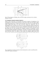
function values indicated that solution (a) with function value of 6.8x10
3
(iteration 5000 and
number of gains before stop 200) is better than solution (b) with function value 6.1x10
3
(iteration 1000, number of gains before stop 100). The solutions were obtained in 6 seconds
and 2 seconds respectively. Hence it is possible to obtain faster solutions in real time by
dynamically tuning the GA parameters based on required function value or number of
iterations, and also using a faster computer for running the algorithm. It is however not
clear how the function value varies with different shapes and parameter values. In future,
we hope to study how to adjust the GA parameters dynamically to obtain the fastest
solutions in real time.
(a) (b)
Figure 9. (a-b) Finger points for the same object for different functional values
7. Conclusion
The main contributions of this research are an effective vision based method to compute the
optimal grasp points for a 2D prismatic object using GA has been proposed. The simulation
and experimental results prove that it is possible to apply the algorithm in practical cases to
find the optimal grasp points. In future we hope to integrate the method in a multifinger
robotic hand to grasp different types of deforming objects autonomously.
8. References
Bicchi, A. & Kumar, V. (2000). Robot Grasping and Control: A review, Proceedigns of the IEEE
International Conference on Robotics and Automation, pp. 348-353, ISSN 1050 4729.
Blake, A. (1995). A symmetric theory of planar grasp, The International Journal of Robotics
Research, vol. 14, no. 5, pp. 425-444, ISSN 0278-3649.
Chinellato, E., Fisher, R.B., Morales, A. & del Pobil, A. P. (2003). Ranking planar grasp
configurations for a three finger hand, Proceedings of the IEEE International
Conference on Robotics and Automation, pp. 1133-1138, ISSN 1050 4729.

Gatla, C., Lumia, R., Wood, J. & Starr, G.(2004). An efficient method to compute three
fingered planar object grasps using active contour models, Proceedigns of the
IEEE/RSJ International Conference on Intelligent Robots and Systems, pp. 3674-3679,
ISBN 07803-8463-6.
Gordy, M. (1996) A Matlab routine for function maximization using Genetic Algorithm.
Matlab Codes: GA.
Hirai, S., Tsuboi, T. & Wada, T. (2001) Robust grasping manipulation of deformable objects,
Proceedings of the IEEE International Conference on Assembly and Task Planning, pp.
411-416, ISBN 07803-7004.
Vision Systems: Applications 32
Sharma, P., Saxena, A. & Dutta, A. (2006). Multi agent form closure capture of a generic 2D
polygonal object based on projective path planning, Proceedings of the ASME 2006
International Design Engineering Technical Conferences, pp.1-8, ISBN 07918-3784.
Mishra T., Guha, P., Dutta, A. & Venkatesh K. S. (2006). Efficient continuous re-grasp
planning for moving and deforming planar objects, Proceedings of the IEEE
International Conference on Robotics and Automation, pp. 2472 – 2477, ISSN 1050 4729.
Mirtich, B. & Canny, J. (1994). Easily computable optimum grasps in 2D and 3D, Proceedings
of the IEEE International Conference on Robotics and Automation, pp. 739-747.
Nguyen, V.D. (1989). Constructing stable force-closure grasps, International Journal of
Robotics Research, vol. 8, no. 1, pp. 26-37, 0278-3649.
Yoshikawa, T. (1996). Passive and active closures by constraining mechanisms, Proceedings of
the IEEE International Conference on Robotics and Automation, pp. 1477-1484, ISBN
07803-2988.
3
Multi-Focal Visual Servoing Strategies
Kolja Kühnlenz and Martin Buss
Institute of Automatic Control Engineering (LSR), Technische Universität München
Germany
1. Introduction
Multi-focal vision provides two or more vision devices with different fields of view and

measurement accuracies. A main advantage of this concept is a flexible allocation of these
sensor resources accounting for the current situational and task performance requirements.
Particularly, vision devices with large fields of view and low accuracies can be used
together. Thereby, a coarse overview of the scene is provided, e.g. in order to be able to
perceive activities or structures of potential interest in the local surroundings. Selected
smaller regions can be observed with high-accuracy vision devices in order to improve task
performance, e.g. localization accuracy, or examine objects of interest. Potential target
systems and applications cover the whole range of machine vision from visual perception
over active vision and vision-based control to higher-level attention functions.
This chapter is concerned with multi-focal vision on the vision-based feedback control level.
Novel vision-based control concepts for multi-focal active vision systems are presented. Of
particular interest is the performance of multi-focal approaches in contrast to conventional
approaches which is assessed in comparative studies on selected problems.
In vision-based feedback control of the active vision system pose, several options to make
use of the individual vision devices of a multi-focal system exist: a) only one of the vision
devices is used at a time by switching between the vision devices, b) two or more vision
devices are used at the same time, or c) the latter option is combined with individual
switching of one or several of the devices. Major benefit of these strategies is an
improvement of the control quality, e.g. tracking performance, in contrast to conventional
methods. A particular advantage of the switching strategies is the possible avoidance of
singular configurations due to field of view limitations and an instantaneous improvement
of measurement sensitivity which is beneficial near singular configurations of the visual
controller and for increasing distances to observed objects. Another advantage is the
possibility to dynamically switch to a different vision device, e.g. in case of sensor
breakdown or if the one currently active is to be used otherwise.
The chapter is organized as follows: In Section 2 the general configuration, application areas,
data fusion approaches, and measurement performance of multi-focal vision systems are
discussed; the focus of Section 3 are vision-based strategies to control the pose of multi-focal
active vision systems and comparative evaluation studies assessing their performance in
contrast to conventional approaches; conclusions are given in Section 4.

Vision Systems: Applications 34
Figure 1. Schematical structure of a general multi-focal vision system consisting of several
vision devices with different focal-lengths; projections of a Cartesian motion vector into the
image planes of the individual vision devices
2. Multi-Focal Vision
2.1 General Vision System Structure
A multi-focal vision system comprises several vision devices with different fields of view
and measurement accuracies. The field of view and accuracy of an individual vision device
is mainly determined by the focal-length of the optics in good approximation and by the
size and quantization (pixel sizes) of the sensor-chip. Neglecting the gathered quantity of
light, choosing a finer quantization has approximately the same effect as choosing a larger
focal-length. Therefore, sensor quantization is considered fixed and equal for all vision
devices in this chapter. The projections of an environment point or motion vector on the
image planes of the individual vision devices are scaled differently depending on the
respective focal-lengths. Figure 1 schematically shows a general multi-focal vision system
configuration and the projections of a motion vector.
2.2 Systems and Applications
Cameras consisting of a CCD- or CMOS-sensor and lens or mirror optics are the most
common vision devices used in multi-focal vision. Typical embodiments of multi-focal
vision systems are foveated (bi-focal) systems of humanoid robots with two different cameras
combined in each eye which are aligned in parallel, e.g. (Brooks et al., 1999; Ude et al., 2006;
Vijayakumar et al., 2004). Such systems are the most common types of multi-focal systems.
Systems for ground vehicles, e.g. (Apostoloff & Zelinsky, 2002; Maurer et al., 1996) are
another prominent class whereas the works of (Pellkofer & Dickmanns, 2000) covering
situation-dependent coordination of the individual vision devices are probably the most
advanced implementations known. An upcoming area are surveillance systems which
strongly benefit from the combination of large scene overview and selective observation
with high accuracy, e.g. (Bodor et al., 2004; Davis & Chen, 2003; Elder et al., 2004; Jankovic &
Naish, 2005; Horaud et al., 2006).
An embodiment with independent motion control of three vision devices and a total of 6

degrees-of-freedom (DoF) is the camera head of the humanoid robot L
OLA developed at our
laboratory which is shown in Figure 2, cf. e.g. (Kühnlenz et al., 2006). It provides a flexible
allocation of these vision devices and, due to directly driven gimbals, very fast camera
saccades outperforming known systems.
image plane
motion vector
focal-point
projection ray
optical axis
Multi-Focal Visual Servoing Strategies 35
Most known methods for active vision control in the field of multi-focal vision are
concerned with decision-based mechanisms to coordinate the view direction of a telephoto
vision device based on evaluations of visual data of a wide-angle device. For a survey on
existing methods cf. (Kühnlenz, 2007).
Figure 2. Multi-focal vision system of humanoid LOLA (Kühnlenz et al., 2006)
2.3 Fusion of Multi-Focal Visual Data
Several options exist in order to fuse the multi-resolution data of a multi-focal vision system:
on pixel level, range-image or 3D representation level, and on higher abstraction levels, e.g.
using prototypical environment representations. Each of these is covered by known
literature and a variety of methods are known. However, most works do not explicitly
account for multi-focal systems. The objective of the first two options is the 3D
reconstruction of Cartesian structures whereas the third option may also cover higher-level
information, e.g. photometric attributes, symbolic descriptors, etc.
The fusion of the visual data of the individual vision devices on pixel level leads to a
common multiple view or multi-sensor data fusion problem for which a large body of
literature exists, cf. e.g. (Hartley & Zisserman, 2000; Hall & Llinas, 2001). Common tools in
this context are, e.g., projective factorization and bundle adjustment as well as multi-focal
tensor methods (Hartley & Zisserman, 2000). Most methods allow for different sensor
characteristics to be considered and the contribution of individual sensors can be weighted,

e.g. accounting for their accuracy by evaluating measurement covariances (Hall & Llinas,
2001).
In multi-focal vision fusion of range-images requires a representation which covers multiple
accuracies. Common methods for fusing range-images are surface models based on
triangular meshes and volumetric models based on voxel data, cf. e.g. (Soucy & Laurendeau,
1992; Dorai et al., 1998; Sagawa et al., 2001). Fusion on raw range-point level is also
common, however, suffers from several shortcomings which render such methods less
suited for multi-focal vision, e.g. not accounting for different measurement accuracies.
Several steps have to be accounted for: detection of overlapping regions of the images,
establishment of correspondences in these regions between the images, integration of
corresponding elements in order to obtain a seamless and nonredundant surface or
volumetric model, and reconstruction of new patches in the overlapping areas. In order to
optimally integrate corresponding elements, the different accuracies have to be considered
(Soucy & Lauredau, 1995), e.g. evaluating measurement covariances (Morooka &
Vision Systems: Applications 36
Nagahashi, 2006). The measurement performance of multi-focal vision systems has recently
been investigated by (Kühnlenz, 2007).
2.4 Measurement Performance of Multi-Focal Vision Systems
The different focal-lengths of the individual vision devices result in different abilities
(sensitivities) to resolve Cartesian information. The combination of several vision devices
with different focal-lengths raises the question on the overall measurement performance of
the total system. Evaluation studies for single- and multi-camera configurations with equal
vision device characteristics have been conducted by (Nelson & Khosla, 1993) assessing the
overall sensitivity of the vision system. Generalizing investigations considering multi-focal
vision system configurations and first comparative studies have recently been conducted in
our laboratory (Kühnlenz, 2007).
Figure 3. Qualitative change of approximated sensitivity ellipsoids of a two-camera system
observing a Cartesian motion vector as measures to resolve Cartesian motion; a) two wide-
angle cameras and b) a wide-angle and a telephoto camera with increasing stereo-base,
c) two-camera system with fixed stereo-base and increasing focal-length of upper camera

The multi-focal image space can be considered composed of several subspaces
corresponding to the image spaces of the individual vision devices. The sensitivity of the
multi-focal mapping of Cartesian to image space coordinates can be approximated by an
ellipsoid. Figure 3a and 3b qualitatively show the resulting sensitivity ellipsoids in Cartesian
space for a conventional and a multi-focal two-camera system, respectively, with varied
distances between the cameras. Two main results are pointed out: Increasing the focal-
length of an individual vision device results in larger main axes of the sensitivity ellipsoid
and, thus, in improved resolvability in Cartesian space. This improvement, however, is
nonuniform in the individual Cartesian directions resulting in a weaker conditioned
mapping of the multi-focal system. Another aspect shown in Figure 3c is an additional
rotation of the ellipsoid with variation of the focal-length of an individual vision device.
This effect can also be exploited in order to achieve a better sensitivity in a particular
direction if the camera poses are not variable.
a) b)
c)
focal-len
g
th
Multi-Focal Visual Servoing Strategies 37
In summary, multi-focal vision provides a better measurement sensitivity and, thus, a
higher accuracy, but a weaker condition than conventional vision. These findings are
fundamental aspects to be considered in the design and application of multi-focal active
vision systems.
3. Multi-Focal Active Vision Control
3.1 Vision-Based Control Strategies
Vision-based feedback control, also called visual servoing, refers to the use of visual data
within a feedback loop in order to control a manipulating device. There is a large body of
literature which is surveyed in a few comprehensive review articles, e.g. cf. (Chaumette et
al., 2004; Corke, 1994; Hutchinson et al., 1996; Kragic & Christensen, 2002). Many
applications are known covering, e.g., basic object tracking tasks, control of industrial

robots, and guidance of ground and aerial vehicles.
Most approaches are based on geometrical control strategies using inverse kinematics of
robot manipulator and vision device. Manipulator dynamics are rarely considered. A
commanded torque is computed from the control error in image space projected into
Cartesian space by the image Jacobian and a control gain.
Several works on visual servoing with more than one vision device allow for the use of
several vision devices differing in measurement accuracy. These works include for instance
the consideration of multiple view geometry, e.g. (Hollighurst & Cipolla, 1994; Nelson &
Khosla, 1995; Cowan, 2002) and eye-in-hand/eye-to-hand cooperation strategies, e.g.
(Flandin et al., 2000; Lipiello et al., 2005). A more general multi-camera approach is (Malis et
al., 2000) introducing weighting coefficients of the individual sensors to be tuned according
to the multiple sensor accuracies. However, no method to determine the coefficients is
given. Control in invariance regions is known resulting in independence of intrinsic camera
parameters and allowing for visual servoing over several different vision devices, e.g.
(Hager, 1995; Malis, 2001). The use of zooming cameras for control is also known, e.g.
(Hayman, 2000; Hosoda et al., 1995), which, however, cannot provide both, large field of
view and high measurement accuracy, at the same time.
Multi-focal approaches to visual servoing have recently been proposed by our laboratory in
order to overcome common drawbacks of conventional visual servoing (Kühnlenz & Buss,
2005; Kühnlenz & Buss, 2006; Kühnlenz, 2007). Main shortcomings of conventional
approaches are dependency of control performance on distance between vision device and
observed target and limitations of the field of view. This chapter discusses three control
strategies making use of the individual vision devices of a multi-focal vision system in
various ways. A switching strategy dynamically selects a particular vision device from a set
in order to satisfy conditions on control performance and/or field of view, thereby, assuring
a defined performance over the operating distance range. This sensor switching strategy
also facilitates visual servoing if a particular vision device has to be used for other tasks or in
case of sensor breakdown. A second strategy introduces vision devices with high accuracy
observing selected partial target regions in addition to wide-angle devices observing the
remaining scene. The advantages of both sensor types are combined: increase of sensitivity

resulting in improved control performance and the observation of sufficient features in
order to avoid singularities of the visual controller. A third strategy combines both strategies
allowing independent switches of individual vision devices simultaneously observing the
scene. These strategies are presented in the following sections.
Vision Systems: Applications 38
3.2 Sensor Switching Control Strategy
A multi-focal active vision system provides two or more vision devices with different
measurement accuracies and fields of view. Each of these vision devices can be used in a
feedback control loop in order to control the pose of the active vision system evaluating
visual information. A possible strategy is to switch between these vision devices accounting
for requirements on control performance and field of view or other situation-dependent
conditions. This strategy is discussed in the current section.
Figure 4. Visual servoing scenario with multi-focal active vision system consisting of a wide-
angle camera (h
1
) and a telephoto camera (h
2
); two vision system poses with switch of active
vision device
The proposed sensor switching control strategy is visualized in Figure 5. Assumed is a
physical vision device mapping observed feature points concatenated in vector r to an
image space vector
ξ
))(,( qxrh=
ξ
, (1)
at some Cartesian sensor pose x relative to the observed feature points which is dependent
on the joint angle configuration q of the active vision device. Consider further a velocity
relationship between image space coordinates
ξ

and joint space coordinates q
qqqJq


)),(()(
ξξ
=
, (2)
with differential kinematics J=J
v
RJ
g
corresponding to a particular combination of vision
device and manipulator, visual Jacobian J
v
, matrix R=diag(R
c
,…,R
c
) with rotation matrix R
c
of camera frame with respect to robot frame, and the geometric Jacobian of the manipulator
J
g
, cf. (Kelly et al., 2000). A common approach to control the pose of an active vision system
evaluating visual information is a basic resolved rate controller computing joint torques
from a control error
ξ
d
-

ξ
(t) in image space in combination with a joint-level controller
gqKKJ
v
d
p
+−−=
+

)(
ξξτ
, (3)
with positive semi-definite control gain matrices K
p
and K
v
, a desired feature point
configuration
ξ
d
, joint angles q, gravitational torques g, and joint torques
τ
. The computed
torques are fed into the dynamics of the active vision system which can be written
τ
=++ )(),()( qgqqqCqqM

, (4)
with the inertia matrix M and C summarizing Coriolis and friction forces, gravitational
torques g, joint angles q, and joint torques

τ
.
h
1
h
2
Multi-Focal Visual Servoing Strategies 39
Now consider a set of n vision devices H={h
1
,h
2
,…,h
n
} mounted on the same manipulator
and the corresponding set of differential kinematics J={J
1
,J
2
,…,J
n
}. An active vision controller
is proposed which substitutes the conventional visual controller by a switching controller
gqKKJ
v
d
p
+−−=
+

)(

ξξτ
η
, (5)
with a switched tuple of vision device h
η
and corresponding differential kinematics J
η
>∈∈< HJ
ηη
hJ ,
,
}, 2,1{ n∈
η
, (6)
selected from the sets J and H.
Figure 5. Block diagram of multi-focal switching visual servoing strategy; vision devices are
switched directly or by conditions on field of view and/or control performance
This switching control strategy has been shown locally asymptotically stable by proving the
existence of a common Lyapunov function under the assumption that no parameter
perturbations exist (Kühnlenz, 2007). In case of parameter perturbations, e.g. focal-lengths
or control gains are not known exactly, stability can be assured by, e.g., invoking multiple
Lyapunov functions and the dwell-time approach (Kühnlenz, 2007).
A major benefit of the proposed control strategy is the possibility to dynamically switch
between several vision devices if the control performance decreases. This is, e.g., the case at
or near singular configurations of the visual controller. Most important cases are the
exceedance of the image plane limits by observed feature points and large distances
between vision device and observed environmental structure. In these cases a vision device
with a larger field of view or a larger focal-length, respectively, can be selected.
Main conditions for switching of vision devices and visual controller may consider
requirements on control performance and field of view. A straight forward formulation

dynamically selects the vision device with the highest necessary sensitivity in order to
provide a sufficient control performance, e.g. evaluating the pose error variance, in the
current situation. As a side-condition field of view requirements can be considered, e.g.
always selecting the vision device providing sufficient control performance with maximum
field of view. Alternatively, if no measurements of the vision device pose are available the
sensitivity or condition of the visual controller can be evaluated. A discussion of selected
switching conditions is given in (Kühnlenz, 2007).
manipulator
dynamics /
forward
kinematics
J
1+
J
n+
. . .
K
p
K
v
g
h
1
h
n
switching
condition
. . .
field of view
performance

sensor selector
ξ
d
x
ξ
q
q
.
τ
Vision Systems: Applications 40
3.3 Comparative Evaluation Study of Sensor Switching Control Strategy
The impact of the proposed switching visual servoing strategy on control performance is
evaluated in simulations using a standard trajectory following task along the optical axis.
The manipulator dynamics are modeled as a simple decoupled mass-damper-system.
Manipulator geometry is neglected. Joint and Cartesian spaces are, thus, equivalent. The
manipulator inertia matrix is M=0.05diag(1kg, 1kg, 1kg, 1kgm
2
, 1kgm
2
, 1kgm
2
) and matrices
K
v
+C=0.2diag(1kgs
-1
, 1kgs
-1
, 1kgs
-1

, 1kgms
-1
, 1kgms
-1
, 1kgms
-1
). The control gain K
p
is set
such that the system settles in 2s for a static
ξ
d
. A set of three sensors with different focal-
lengths of H={10mm, 20mm, 40mm} and a set of corresponding differential kinematics
J={J
1
, J
2
, J
3
} based on the visual Jacobian are defined. The vision devices are assumed
coincident. A feedback quantization of 0.00001m and a sensor noise power of 0.00001
2
m
2
are
assumed. A square object is observed with edge lengths of 0.5m at an initial distance of 1m
from the vision system. The desired trajectory is
T
d

tttx
»
¼
º
«
¬
ª
−
¸
¹
·
¨
©
§
−=
5
1
00
2
7
25
1
sin
2
7
00)(
π
, (7)
with a sinusoidal translation along the optical axes and a uniform rotation around the
optical axes. The corresponding desired feature point vector

ξ
d
is computed using a pinhole
camera model.
í0.2
0
0.2
a)
e
pose,i
[m,rad]
í0.2
0
0.2
b)
e
pose,i
[m,rad]
í0.2
0
0.2
c)
e
pose,i
[m,rad]
0 5 10 15 20 25 30
í10
0
10
t [s]

d
)
x
pose,i
[m,rad]
e
e
φ,z
z
e
φ,z
e
φ,z
e
z
e
z
x
φ,z
x
z
Figure 6. Tracking errors e
pose,i
and trajectory x
pose,i
of visual servoing trajectory following
task; sinusoidal translation along optical (x
z
-)axis with uniform rotation (x
φ

,z
) ; focal-lengths
a) 10mm, b) 20mm, c) 40mm
For comparison the task is performed with each of the vision devices independently and
afterwards utilizing the proposed switching strategy. A switching condition is defined with
Multi-Focal Visual Servoing Strategies 41
a pose error variance band of σ
2
=6.25 10
-6
m
2
and a side-condition to provide a maximum
field of view. Thus, whenever this variance band is exceeded the next vision device
providing the maximum possible field of view is selected.
0 5 10 15 20 25 30
0
0.005
0.01
0.015
0.02
t [s]
σ
e,z
[m]
λ=10mm
λ=20mm
λ=40mm
Figure 7. Corresponding tracking error standard deviation estimates for trajectory following
tasks (Figure 6) with different cameras; three samples estimation window

í0.1
0
0.1
a)
e
pose,i
[m,rad]
0
0.01
0.02
b)
σ
e,z
[m]
10
20
40
c)
λ [mm]
0 5 10 15 20 25 30
í10
0
10
t [s]
d
)
x
pose,i
[m,rad]
e

φ,z
e
z
x
φ,z
x
z
Figure 8. Results of sensor switching visual servoing strategy with multi-focal vision;
sinusoidal translation along optical (x
z
-)axis with uniform rotation (x
φ
,z
); a) tracking errors,
b) tracking error standard deviation estimates, c) current focal-length, d) pose trajectory
Figure 6 shows the resulting tracking errors for the trajectory following task for each of the
individual vision devices. In spite of very low control error variances in image space of
about 0.01 pixels
2
large pose error variances in Cartesian space can be noted which vary
over the whole operating distance as shown in Figure 7. The distance dependent sensitivity
of the visual controller and quantization effects result in varying pose error variances over
the operating range caused by sensor noise. These effects remain a particular problem for
wide range visual servoing rendering conventional visual servoing strategies unsuitable.
Vision Systems: Applications 42
Figure 8 shows the results of the switching control strategy. The standard deviation (Figure
8b) is kept within a small band reaching from about 0.004m to 0.008m. The overall
variability is significantly lower compared to the single-camera tasks (Figure 7). The spikes,
which can be noted in the standard deviation diagram, are caused by the switches due to the
delay of the feedback signal. After a switch the desired feature value changes with the

sensor, but the current value is still taken from the previous sensor. Thus, the control error
at this time instance jumps. This effect can be reduced by mapping the previous value of the
feature vector to the image space of the new sensor or by definition of a narrower variance
band as switching condition.
Figure 9 exemplarily illustrates the progression of the fields of view over time for a uniform
single-camera translation task and the corresponding camera switching task. The field of
view is defined by the visible part of the plane extending the surface of the observed object
in x-direction. The variability achieved with the switching strategy is significantly lower.
The effectiveness of the proposed multi-focal switching strategy has been shown
successfully. The contributions of this novel approach are a guaranteed control performance
by means of a bounded pose error variance, a low variability of the performance over the
whole operating range, and the consideration of situational side-conditions as, e.g., a
maximum field of view.
3.4 Multi-Camera Control Strategy
If two or more vision devices of a multi-focal system are available simultaneously these
devices can be used together in order to control the pose of the vision system. In this section
a multi-focal multi-camera strategy is proposed in order to make use of several available
vision devices with different fields of view and measurement accuracies. Major benefit is an
improved control performance compared to single-camera strategies whereas only a partial
observation of the reference object with high accuracy is necessary.
0
2
4
a)
FOV [ m ]
0 5 10 15 20 25 30
í10
í5
0
5

t[s]
x
pose,i
[m]
0
2
4
b)
FOV [ m ]
λ=10mm
λ=20mm
λ=40mm
xx
x
z
Figure 9. Progression of the extension of the field of view orthogonal to the optical axis of
the observing vision device; uniform translation along optical (x
z
-)axis; a) single-camera
tasks, b) sensor switching strategy with multi-focal vision, c) pose trajectory
Multi-Focal Visual Servoing Strategies 43
A vision-based controller computing joint torques from a control error in image space
requires sufficient observed feature points to be mapped to the six Cartesian degrees of
freedom. A minimum of three feature points composed of two elements in image space is
needed in order to render the controller full rank. If the field of view of the observing vision
device is too small to cover all feature points the controller becomes singular. However,
high-sensitivity sensors needed in order to achieve high control performance only provide
small fields of view.
A multi-camera strategy is proposed combining the advantages of vision devices with
different characteristics. High-sensitivity devices are used for improving control

performance and wide-field-of-view devices in order to observe the required number of
remaining feature points to render the controller full rank.
Figure 10. Visual servoing scenario with multi-focal active vision system consisting of a
wide-angle camera (h
1
) and a telephoto camera (h
2
); both vision devices are observing
different feature points of a reference object accounting for field of view constraints
The sensor equation (1) extends such that individual feature points are observed with
different vision sensors
[][]
(
)
[]
(
)
[]
T
T
T
j
T
T
i
T
T
T
j
T

i
T
qxrhqxrrh  )(,)(,
221111
=
ξξξ
, (8)
where a Cartesian point r
k
is mapped to an image point
ξ
l
by vision device h
m
. The proposed
visual controller is given by
[]
gqKKJJJ
v
d
p
T
TTT
+−−=
+

 )(
211
ξξτ
, (9)

with image feature vector
ξ
=[
ξ
1
ξ
i
ξ
j
]
T
and differential kinematics J
m
corresponding to
vision device h
m
.
Substituting the composition of individual differential kinematics J
m
by a generalized
differential kinematics J
*
the proposed control strategy can be expressed by
gqKKJ
v
d
p
+−−=
+


)(
*
ξξτ
, (10)
which has been proven locally asymptotically stable (Kelly et al., 2000).
Utilizing the proposed multi-camera strategy an improved control performance is achieved
even though only parts of the observed reference structure are visible for the high-
sensitivity vision devices. This multi-camera strategy can be combined with the switching
h
1
h
2
Vision Systems: Applications 44
strategy discussed in Section 3.2 allowing switches of the individual vision devices of a
multi-focal vision system. Such a multi-camera switching strategy is discussed in the
following section.
3.5 Multi-Camera Switching Control Strategy
In the previous sections two concepts to make use of the individual vision devices of a
multi-focal vision system have been presented: a sensor switching and a multi-camera
vision-based control strategy. This section proposes the integration of both strategies, thus,
allowing switches of one or more vision devices observing parts of a reference structure
simultaneously. Thereby, the benefits of both strategies are combined.
The sensor equation (8) is extended writing
[][]
(
)
[]
(
)
[]

T
T
T
j
T
T
i
T
T
T
j
T
i
T
qxrhqxrrh  )(,)(,
221111
ηη
ξξξ
=
, (11)
allowing the h
m
η
of (8) to be selected dynamically from a set H={h
1
,h
2
,…,h
n
}. The visual

controllers (5) and (10) are integrated writing
gqKKJ
v
d
p
+−−=
+

)(
*
ξξτ
η
, (12)
where J
η∗
is composed of individual differential kinematics J
m
[]
T
TTT
JJJJ 
ηηη
η
211
*
=
+
, (13)
which are selected dynamically from a set J={J
1

,J
2
,…,J
n
} of differential kinematics
corresponding to the set H of available vision devices.
In the following section the proposed multi-camera strategies are exemplarily evaluated in a
standard visual servoing scenario.
3.6 Comparative Evaluation Study of Multi-Camera Control Strategies
In this section a comparative evaluation study is conducted in order to demonstrate the
benefits of the proposed multi-camera and multi-camera switching strategies. Considered is
again a trajectory following task with a uniform translation along the optical axis of a main
camera with a wide field of view (focal-length 5mm) as shown in Figure 10. A square
reference object is observed initially located at a distance of 1m to the camera. A second
camera observes only one feature point of the object. The characteristics of this camera are
switchable. Either the same characteristics as of the wide-angle camera or telephoto
characteristics (focal-length 40mm) are selectable. The inertia matrix is set to M=0.5diag(1kg,
1kg, 1kg, 1kgm
2
, 1kgm
2
, 1kgm
2
) and matrices K
v
+C=200diag(1kgs
-1
, 1kgs
-1
, 1kgs

-1
, 1kgms
-1
,
1kgms
-1
, 1kgms
-1
). The other simulation parameters are set equal to section 3.3.
Three simulation scenarios are compared: second camera with wide-angle characteristics,
with telephoto characteristics, and switchable. Switches of the second camera are allowed
after a time of 2s when a constant tracking error is achieved. A switch is performed when
the tracking error standard deviation exceeds a threshold of 0.00004m.
Figure 11 shows the tracking error of the uniform trajectory following task with switched
second camera which can be considered constant after about 2s. Figure 12 shows the
resulting standard deviations of the tracking error for all three tasks. It can be noted that a
Multi-Focal Visual Servoing Strategies 45
lower standard deviation is achieved by the multi-camera task (second camera with
telephoto characteristics) compared to the wide-angle task. The multi-camera switching task
additionally achieves a lower variability of the standard deviation of the tracking error.
0 0.5 1 1.5 2 2.5 3 3.5 4
0
0.02
0.04
0.06
0.08
0.1
e
pose,z
[m]

t [s]
Figure 11. Tracking error of multi-focal two-camera visual servoing task with wide-angle
and switchable wide-angle/telephoto camera; desired trajectory x
z
d
(t)=-0.2ms
-1
t-1m
0.5 1 1.5 2 2.5 3 3.5 4
0
2
4
6
8
x 10
í5
σ
e,z
[m]
t [s]
multiífocal
wideíangle
multiífocal
swi t ch ed
multi-camera
Figure 12. Standard deviation estimates of tracking error of unswitched single-camera task
(wide-angle), of unswitched multi-focal multi-camera task with one feature point observed
by additional telephoto camera, and of switched multi-focal multi-camera task with
additional camera switching from wide-angle to telephoto characteristics at t=2.6s
0 0.5 1 1.5 2 2.5 3 3.5 4

0
1
2
3
4
5
x 10
í3
s
z
v
z
t [s]
multiífocal
multiífocal
swi t ch ed
wideíangle
multi-camera
Figure 13. Sensitivities of the visual servoing controller along the optical axis of the central
wide-angle camera corresponding to the tasks in Figure 12
Vision Systems: Applications 46
Figure 13 shows the sensitivity (s
z
v
z
) of the visual controller for all three tasks along the
optical axis of the wide-angle camera. It can be noted that the multi-camera strategies result
in a better sensitivity of the controller compared to the wide-angle task.
Summarized, the simulations clearly show the benefits of the proposed multi-camera control
strategies for multi-focal vision systems: an exploitation of the field of view and sensitivity

characteristics in order to achieve improved control performance and a lower variability of
the performance by switching of individual vision devices.
4. Conclusion
In this chapter novel visual servoing strategies have been proposed based on multi-focal
active vision systems able to overcome common drawbacks of conventional approaches: a
tradeoff between field of view and sensitivity of vision devices and a large variability of the
control performance due to distance dependency and singular configurations of the visual
controller. Several control approaches to exploit the benefits of multi-focal vision have been
proposed and evaluated in simulations: Serial switching between vision devices with
different characteristics based on performance- and field-of-view-dependent switching
conditions, usage of several of these vision devices at the same time observing different
parts of a reference structure, and individual switching of one or more of these
simultaneously used sensors. Stability has been discussed utilizing common and multiple
Lyapunov functions.
It has been shown that each of the proposed strategies significantly improves the visual
servoing performance by reduction of the pose error variance. Depending on the
application scenario several guidelines for using multi-focal vision can be given. If only one
vision sensor at a time is selectable then a dynamical sensor selection satisfying desired
performance constraints and side-conditions is proposed. If several vision sensors can be
used simultaneously selected features of a reference object can be observed with high-
sensitivity sensors while a large field of view sensor ensures observation of a sufficient
number of features in order to render the visual controller full rank. The high-sensitivity
sensors should preferably be focused on those feature points resulting in the highest
sensitivity of the controller.
5. Acknowledgments
The authors like to gratefully thank Dr. Nicholas Gans and Prof. Seth Hutchinson for
inspiring discussions and reference simulation code for performance comparison. This work
has been supported in part by the German Research Foundation (DFG) grant BU-1043/5-1
and the DFG excellence initiative research cluster Cognition for Technical Systems - CoTeSys,
see also www.cotesys.org.

6. References
Apostoloff, N. & Zelinsky, A. (2002). Vision in and out of vehicles: Integrated driver and
road scene monitoring, Proceedings of the 8
th
International Symposium on Experimental
Robotics (ISER), 2002, Sant Angelo d’Iscia, Italy
Multi-Focal Visual Servoing Strategies 47
Bodor, R.; Morlok, R. & Papanikolopoulos, N. (2004). Dual-camera system for multi-level
activity recognition, Proceedings of the 2004 IEEE/RSJ International Conference on
Intelligent Robots and Systems (IROS), 2004, Sendai, Japan
Brooks, R. A.; Breazeal, C.; Marjanovic, M.; Scasselati, B. & Williamson, M. M. (1999). The
Cog Project: Building a Humanoid Robot, In: Computation for Methaphors, Analogy,
and Agents, C. Nehaniv, (Ed.), Springer, Germany
Chaumette, F.; Hashimoto, K.; Malis, E. & Martinet, P. (2004). TTP4: Tutorial on Advanced
Visual Servoing, Tutorial Notes, IEEE/RSJ IROS, 2004
Corke, P. I. (1994). Visual Control of Robot Manipulators – A Review, In: Visual Servoing, K.
Hashimoto, (Ed.), World Scientific, 1994
Cowan, N. (2002). Binocular visual servoing with a limited field of view, In: Mathematical
Theory of Networks and Systems, Notre Dame, IN, USA, 2002
Dickmanns, E. D. (2003). An advanced vision system for ground vehicles, Proceedings of the
International Workshop on In-Vehicle Cognitive Computer Vision Systems (IVC2VS),
2003, Graz, Austria
Dorai, C.; Wang, G.; Jain, A. K. & Mercer, C. (1998). Registration and Integration of Multiple
Object Views for 3D Model Construction, In: IEEE Transactions on Pattern Analysis
and Machine Intelligence, Vol. 20, No. 1, 1998
Elder, J. H.; Dornaika, F.; Hou, B. & Goldstein, R. (2004). Attentive wide-field sensing for
visual telepresence and surveillance, In: Neurobiology of Attention, L. Itti, G. Rees & J.
Tsotsos, (Eds.), 2004, Academic Press, Elsevier
Flandin, G.; Chaumette, F. & Marchand, E. (2000). Eye-in-hand/eye-to-hand cooperation for
visual servoing, Proceedings of the IEEE/RSJ International Conference on Intelligent

Robots and Systems (IROS), 2003
Hager, G. D. (1995). Calibration-free visual control using projective invariance, Proceedings of
the 5
th
International Conference on Computer Vision (ICCV), 1995
Hall, D. L. & Llinas, J. (2001). Handbook of Multisensor Data Fusion, CRC Press, 2001, Boca
Raton, FL, USA
Hartley, R. I. & Zisserman, A. (2004). Multiple View Geometry in Computer Vision, Cambridge
University Press, 2004, NY, USA
Hayman, E. (2000). The use of zoom within active vision, Ph.D. Thesis, University of Oxford,
2000, Oxford, UK
Hollighurst, N. & Cipolla, R. (1994). Uncalibrated stereo hand-eye coordination, In: Image
and Vision Computing, Vol.12, No. 3, 1994
Horaud, R.; Knossow, D. & Michaelis, M. (2006). Camera cooperation for achieving visual
attention, In: Machine Vision and Applications, Vol. 15, No. 6, 2006, pp. 331-342
Hosoda, K.; Moriyama, H. & Asada, M. (1995). Visual servoing utilizing zoom mechanism,
Proceedings of the IEEE International Conference on Robotics and Automation (ICRA),
1995
Hutchinson, S.; Hager, G. D. & Corke, P. I. (1996). A tutorial on visual servo control, In: IEEE
Transaction on Robotics and Automation, Vol. 12, No. 5, 1996
Jankovic, N. D. & Naish, M. D. (2005). Developing a modular spherical vision system,
Proceedings of the 2005 IEEE International Conference on Robotics and Automation
(ICRA), pp. 1246-1251, 2005, Barcelona, Spain
Kelly, R.; Carelli, R.; Nasisi, O.; Kuchen, B. & Reyes, F. (2000). Stable visual servoing of camera-
in-hand robotic systems, In: IEEE Transactions on Mechatronics, Vol. 5, No. 1, 2000
Vision Systems: Applications 48
Kragic, D. & Christensen, H. I. (2002). Survey on Visual Servoing for Manipulation, Technical
Report, Stockholms Universitet, ISRN KTH/NA/P-02/01-SE, CVAP259, 2002
Kühnlenz, K. & Buss, M. (2005). Towards multi-focal visual servoing, Proceedings of the
IEEE/RSJ International Conference on Intelligent Robots and Systems (IROS), 2005

Kühnlenz, K. & Buss, M. (2006). A multi-camera view stabilization strategy, Proceedings of the
IEEE/RSJ International Conference on Intelligent Robots and Systems (IROS), 2006
Kühnlenz, K. (2007). Aspects of multi-focal vision, Ph.D. Thesis, Institute of Automatic Control
Engineering, Technische Universität München, 2007, Munich, Germany
Kühnlenz, K.; Bachmayer, M. & Buss, M. (2006). A multi-focal high-performance vision
system, Proceedings of the 2006 IEEE International Conference on Robotics and
Automation (ICRA), 2006, Orlando, FL, USA
Lipiello, V.; Siciliano, B. & Villani, L. (2005). Eye-in-hand/eye-to-hand multi-camera visual
servoing, Proceedings of the IEEE International Conference on Decision and Control
(CDC), 2005
Malis, E. (2001). Visual servoing invariant to changes in camera intrinsic parameters,
Proceedings of the 8
th
International Conference on Computer Vision (ICCV), 2001
Malis, E.; Chaumette, F. & Boudet, S. (2000). Multi-cameras visual servoing, Proceedings of the
IEEE International Conference on Robotics and Automation (ICRA), 2000
Maurer, M.; Behringer, R.; Furst, S.; Thomanek, F. & Dickmanns, E. D. (1996). A compact
vision system for road vehicle guidance, Proceedings of the 13
th
International
Conference on Pattern Recognition (ICPR), 1996
Morooka, K. & Nagahashi H. (2006). A Method for Integrating Range Images in Different
Resolutions for 3-D Model Construction, Proceedings of the IEEE International
Conference on Robotics and Automation (ICRA), 2006
Nelson, B. & Khosla, P. (1993). The resolvability ellipsoid for visually guided manipulation,
Technical Report, CMU-RI-TR-93-28, The Robotics Institute, Carnegie Mellon
University, 1993, Pittsburgh, PA, USA
Nelson, B. & Khosla, P. (1995). An extendable framework for expectation-based visual
servoing using environment models, Proceedings of the IEEE International Conference
on Robotics and Automation (ICRA), 1995

Pellkofer, M. & Dickmanns, E. D. (2000). EMS-Vision: Gaze control in Autonomous vehicles,
Proceedings of the IEEE Intelligent Vehicles Symposium, 2000, Dearborn, MI, USA
Sagawa, R.; Nishino, K. & Ikeuchi, K. (2001). Robust and Adaptive Integration of Multiple
Range Images with Photometric Attributes, Proceedings of the IEEE International
Conference on Computer Vision and Pattern Recognition (CVPR), 2001
Soucy, M. & Laurendeau, D. (1992). Multi-Resolution Surface Modelling from Multiple
Range Views, Proceedings of the IEEE International Conference on Computer Vision and
Pattern Recognition (CVPR), 1992
Ude, A.; Gaskett, C. & Cheng, G. (2006). Foveated Vision Systems with Two Cameras Per
Eye, Proceedings of the 2006 IEEE International Conference on Robotics and Automation
(ICRA), 2006, Orlando, FL, USA
Vijayakumar, S.; Inoue, M. & Souza, A. D. (2004). Maveric – Oculomotor experimental vision
head, 2004
4
Grasping Points Determination Using Visual
Features
Madjid Boudaba
1
, Alicia Casals
2
and Heinz Woern
3
1
Design Center, TES Electronic Solutions GmbH, Stuttgart
2
GRINS: Research Group On Intelligent Robots and Systems,Technical University of
Catalonia, Barcelona
3
Institute of Process Control and Robotics (IPR), University of Karlsruhe
1,3

Germany,
2
Spain
1. Introduction
This paper discusses some issues for generating point of contact using visual features. To
address these issues, the paper is divided into two sections: visual features extraction and
grasp planning. In order to provide a suitable description of object contour, a method for
grouping visual features is proposed. A very important aspect of this method is the way
knowledge about grasping regions are represented in the extraction process, which is used
also as filtering process to exclude all undesirable grasping point (unstable points) and all line
segments that do not fit to the fingertip position. Fingertips are modelled as point contact with
friction using the theory of polyhedral convex cones. Our approach uses three-finger contact
for grasping planar objects. Each set of three candidate of grasping points is formu- lated as
linear constraints and solved using linear programming solvers. Finally, we briefly describe
some experiments on a humanoid robot with a stereo camera head and an anthropomorphic
robot hand within the ”Centre of excellence on Humanoid Robots: Learning and co-operating
Systems” at the University of Karlsruhe and Forchungszentrum Karlsruhe.
2. Related work
Grasping by multi-fingered robot hands has been an active research area in the last years.
Several important studies including grasp planning, manipulation and stability analysis
have been done. Most of these researches assume that the geometry of the object to be
grasped is known, the fingertip touches the object in a point contact without rolling, and the
position of the contact points are estimated based on the geometrical constraints of the 2
Madjid Boudaba, Alicia Casals and Heinz Woern grasping system. These assumptions
reduce the complexity of the mathematical model of the grasp (see [Park and Starr, 1992],
[Ferrari and Canny, 1992], [Ponce and Faverjon, 1995], [Bicchi and Kumar, 2000], [J. W. Li
and Liu, 2003]). A few work, however has been done in integrating vision-sensors for
grasping and manipulation tasks. To place our approach in perspective, we review existence
methods for sensor based grasp planning. The existing literature can be broadly classified in
two categories; vision based and tactile based. For both categories, the extracted image

Vision Systems: Applications
50
features are of concern which are vary from geometric primitives such as edges, lines,
vertices, and circles to optical flow estimates. The first category uses visual features to
estimate the robot’s motion with respect to the object pose [Maekawa et al., 1995], [Smith
and Papanikolopoulos, 1996], [Allen et al., 1999]. Once the robot hands is already aligned
with object, then it needs only to know where the fingers are placed on the object. The
second category of sensor uses tactile features to estimate the touch sensing area that in
contact with the object [Berger and Khosla, 1991], [Chen et al., 1995], [Lee and Nicholls,
1999]. A practical drawback is that the grasp execution is hardly reactive to sensing errors
such as finger positioning errors. A vision sensor, meanwhile, is unable to handle
occlusions. Since an object is grasped according to its CAD model [Koller et al., 1993],
[Wunsch et al., 1997], [Sanz et al., 1998], [N. Giordana and Spindler, 2000], [Kragic et al.,
2001], an image also contains redundant information that could become a source of errors
and ineffciency in the processing.
This paper is an extension of our previous works [Boudaba and Casals, 2005], [Boudaba et
al., 2005], and [Boudaba and Casals, 2006] on grasp planning using visual features. In this
work, we demonstrate its utility in the context of grasp (or fingers) positioning. Consider the
problem of selecting and executing a grasp. In most tasks, one can expect various
uncertainties. To grasp an object implies building a relationship between the robot hand and
object model. The latter is often unavailable or poorly known. So selecting a grasp position
from such model can be unprecise or unpracticable in real time applications. In our
approach, we avoid to use any object model and instead it works directly from image
features. In order to avoid fingers positioning error, a set of grasping regions is defined that
represents the features of grasping contact point. This not only avoids detection/localization
errors but also saves computations that could affect the reliability of the system. Our
approach can play the critical role of forcing the fingers to a desired positions before the task
of grasping is executed.
The proposed work can be highlighted in two major phases:
1. Visual information phase: In this phase, a set of visual features such as object size, center

of mass, main axis for orientation, and object’s boundary are extracted. For the purpose of
grasping region determination, extracting straight segments are of concern using the
basic results from contour based shape representation techniques. We will focus on the
class techniques that attempt to represent object’s contour into a model graph, which
preserves the topological relationships between features.
2. Grasp planning phase:
The grasping points are generated in the planning task taking as
input these visual features extracted from the first phase. So a relationship between
visual features and grasp planning is proposed. Then a set of geometrical functions is
analysed to find a feasible solution for grasping. The result of grasp planning is a
database contains a list of:
• Valid grasps. all grasps that fulfill the condition of grasp.
• Best Grasps. a criterion for measuring a grasp quality is used to evaluate the best
grasps from a list of valid grasps.
• Reject grasps. those grasps that do not fulfill the condition of grasp.
The remainder of this chapter is organized as follows: Section 3 gives some background for
grasping in this direction. The friction cone modeling and condition of force-closure grasps
are discussed. In section 4, a vision system framework is presented. The vision system is
divided into two parts: the first part concerning to 2D grasping and the second part
Grasping Points Determination Using Visual Features
51
concerning 3D grasping. we first discuss the extracted visual information we have
integrated in grasp planning, generation of grasping regions by using curves fitting and
merging techniques, and discuss the method of selecting valid grasps using the condition of
force-closure grasp. We then discuss the algorithm for computing feasible solutions for
grasping in section 5. We verify our algorithm by presenting experimental results of 2D
object grasping with three-fingers. Finally, we discuss the result of our approach, and future
work in section
6.
3. Grasp Background

Our discussion is based on [Hirai, 2002]. Given a grasp which is characterized by a set of
contact points and the associated contact models, determine if the grasp has a force-closure.
For point contact, a commonly used model is point contact with friction (PCWF). In this
model, fingers can exert any force pointing into friction cone at the edge of contacts (We use
edge contact instead of point contact and can be described as the convex sum of proper
point contacts). To fully analyze the grasp feasibility, we need to examine the full space of
forces acting on the object. Forming the convex hull of this space is diffcult due to the
nonlinear friction cone constraints imposed by the contact models. In this section, we only
focus in precision grasps, where only the fingertips are in contact with the object. After
discussing the friction cone modeling, a formalizme is used for analysing the force closure
grasps using the theory of polyhedral convex cones.
3.1 Modeling the Point of Contact
A point of contact with friction (sometimes referred to as a hard-finger) im- poses non linear
constraints on the force inside of its friction cones. For the analysis of the contact forces in
planar grasps, we simplify the problem by modeling the friction cones as a convex
polytopes using the theory of polyhedral convex cones attributed to [Goldman and Tucker,
1956]. In order to construct the convex polytope from the primitive contact forces, the
following theorem states that a polyhedral convex cone (PCC) can be generated by a set of
basic directional vectors.
(a) (b)
Figure 1. Point Contact Modelling
Theorem 1. A convex cone is a polyhedral if and only if it is finitely generated, that is, the
cone is generated by a finite number of vectors
:
(1)
Vision Systems: Applications
52
where the coeffcients
i
are all non negative. Since vectors u

i
through u
m
span the cone, we
write 1 simply by C=span {u
1
, u
2
, , u
m
}. The cone spanned by a set of vectors is the set of all
nonnegative linear combinations of its vectors. A proof of this theorem can be found in
[Goldman and Tucker, 1956].
Given a polyhedral convex set C, let vert(P)={u
1
, u
2
, , u
m
} stand for vertices of a polytope P,
while face(P)={F
1
, , F
M
} denotes its faces. In the plane, a cone has the appearance as shown
in Figure 1(b). This means that we can reduce the number of cone sides, m = 6 to one face, C
i
.
Let’s denote by P, the convex polytopes of a modelled cone, and {u
1

, u
2
, u
3
} its three vertices.
We can define such polytope as
(2)
where u
i
denotes the i-th vertex of P, and up is the total number of vertices.
n=2 in the case of a 2D plane.
3.2 Force-Closure Grasps
The force-closure of a grasp is evaluated by analysing its convex cone. For a set of friction
cone intersection, the full space can be defined by
(3)
where k is the number of grasping contacts. Note that the result of
is a set of polytopes
intersections and produces either an empty set or a bounded convex polytopes. Therefore,
the solution of (3) can be expressed in terms of its extreme vertices
(4)
where
p
is the total number of extreme vertices.
(a) (b)
Figure 2. Feasible solution of a three-fingered grasp
Figure 2 illustrates an example of feasible solution of and its grasp space represented
by its extreme vertices P = {
}. From this figure, two observations can be
Grasping Points Determination Using Visual Features
53

suggested: first, if the location of a fingertip is not a solution to the grasp, it is possible to move
along its grasping region. Such displacement is defined by u
i
= u
i0
+ ǃ
i
t
i
where ǃ
i
is constrained
by 0  ǃ
i
 l
i
and u
i
be a pointed vertex of C
i
. Second, we define a ray passing through the
pointed vertex u
i
, by a function . The vector
ci
=[
cix
,
ciy
] R

2
varies from the
lower to the upper side of the spanned cone C
i
. This allows us to check whether the feasible
solution remains for all v
ci
in the cone spanned by u
2
and u
3
(see Figure 1(b)).
Testing the force-closure of a grasp now becomes the problem of finding the solutions to (4).
In other words, finding the parameters of (3) that the (4) is a bounded convex polytopes.
4. System Description
We are currently developing a robotic system that can operate autonomously in an
unknown environment. In this case, the main objective is the capability of the system to (1)
locate and measure objects, (2) plan its own actions, and (3) self adaptable grasping
execution. The architecture of the whole system is organized into several modules, which
are embedded in a distributed object communication framework. There are mainly three
modules which are concerned in this development: the extraction of visual information and
its interpretation, grasp planning using the robot hand, the control and execution of grasps
(a) Experimental setup (b) Stereo vision head
Figure 3. Robotic system framework. (a) An humanoid robot arm (7DOF) and an
antropomorphic robot hand (10DOF). (b) Stereo vision system
4.1 The Robot Hand
The prototype of the anthropomorphic robot hands (see [Schulz et al. 2001]) has a 7 degrees
of freedom (DOF) arm (see Fig. 3(a)). This first prototype is currently driven pneumatically
and is able to control the 10 DOF separately, but the joints can only be fully opened or
closed. The robot's task involve controlling the hand for collision-free grasping and

manipulation of objects in the three dimensional space. The system is guided solely by
visual information extracted by the vision system.
Vision Systems: Applications
54
4.2 The Vision System
The vision system shown in Fig. 3(b) consists of a stereo camera (MEGA-D from Videre
Design) mounted on pan-tilt heads equipped with a pair of 4.8 mm lenses and has a fixed
baseline of about 9 cm. The pan-tilt head provides two additional degrees of freedom for the
cameras, both of them rotational. The MEGA-D stereo head uses a IEEE 1394 firewire
interface to connect to a workstation and has a SRI's Small Vision System (SVS) software for
calibration and stereo correlation (see [Konolige, 1997]).
For its complexity, the flow diagram of visual information has been divided into two parts.
The first part provides details of 2D visual features extraction. The second part is dedicated
to 3D visual features retrieval. The image acquisition primarily aims at the conversion of
visual information to electrical signals, suitable for computer interfacing. Then, the incoming
image is subjected to processing having in mind two purposes: (1) removal of image noise
via low-pass filtering by using Gaussian filters due to its computational simplicity and (2)
extraction of prominent edges via high-pass filtering by using the Sobel operator. This
information is finally used to group pixels into lines, or any other edge primitive (circles,
contours, etc). This is the basis of the extensively used Canny's algorithm [Canny, 1986]. So,
the basic step is to identify the main pixels that may preserve the object shape. As we are
visually determining grasping points, the following sections provide some details of what
we need for our approach.
Contour Based Shape Representation
Due to their semantically rich nature, contours are one of the most commonly used shape
descriptors, and various methods for representing the contours of 2D objects have been
proposed in the literature [Costa and Cesar, 2001]. Extracting meaningful features from
digital curves, finding lines or segments in an image is highly significant in grasping
application. Most of the available methods are variations of the dominant point detection
algorithms [M. Marji, 2003]. The advantage of using dominant points is that both, high data

compression and feature extraction can be achieve. Other works prefer the method of
polygonal approximation using linking and merging algorithms [Rosin, 1997] and curvature
scale space (CSS) [Mokhtarian and Mackworth, 1986].
A function regrouping parameters of visual features together can be defined by
(5)
where
is a list of consecutive contour’s vertices with =(x
i
, y
i
) that
represents the location of
relative to the center of mass of the object, com=(x
c
, y
c
). slist={s
1
,
s
2
, · · · , s
m
} is a list of consecutive contour’s segments. Both lists and slist are labelled
counter-clockwise (ccw) order about the center of mass. During the processing, the
boundary of the object, B is maintained as a doubly linked list of vertices and intervening
segments as . The first segment s
1
, connecting vertices
1

and
2
, the last
segment s
m
, connecting vertices
m
and
1
. A vertex
i
is called reflex if the internal angle at
i
is greater than 180 degrees, and convex otherwise. llist is a list that contains the
parameters of correspondent segments. Additional to the local features determined above,
an algorithm for contour following is integrated. This algorithm follows the object’s
boundary from a starting point determined previously and goes counter-clockwise around
the contour by ordering successively its vertices/edge points into a double linked list. The
algorithm stops when the starting point is reached for the second time. The aim of this stage
Grasping Points Determination Using Visual Features
55
is to determine that all vertices/segments belong to the object’s boundary which we will
need further for the determination of the grasping points position.
(a) (b)
(a) Binary object
(a) (b)
(b) Visual features extraction
Figure 4. Object shape representation. (a) Images from original industrial objects
(b) Extraction of grasping regions
Extraction of Grasping Regions

Grasping regions are determined by grouping consecutive edge points from a binary edge
image. This is usually a preliminary step before grasping takes place, and may not be as
time critical as the task of grasping points determination. We deal with (5), the list
is the result that forms an ordered list of connected boundary vertices.
We then need to store the parameters of these primitives instead of discrete points (or
vertices) to fit a line segment to a set of vertices points that lie along a line segment. The aim
of this step is to determine all salient segments that preserve the shape of the object contour.
Figure 4(b) shows grasp regions on the object’s contour. Afterwards, each grasping region is
extracted as straight segment. The size of the grasping regions should be long enough for
positioning the robot fingers. The curve fitting (as shown in Figure 5(a)) describes the
process of finding a minimum set of curve segments to approximate the object’s contour to a
set of line segments with minimum distortion. Once the line segments have been
approximated, the merging method (as shown in Figure 5(b)) is used to merge two lines
segment that satisfied the merging threshold.