243

Inelastic and
Thermoinelastic Materials

19.1 PLASTICITY

Plasticity and thermoplasticity are topics central to the analysis of important appli-
cations, such as metal forming, ballistics, and welding. The main goal of this section
is to present a model of plasticity and thermoplasticity, along with variational and
finite-element statements, accommodating the challenging problems of finite strain
and kinematic hardening.

19.1.1 K

INEMATICS

Elastic and plastic deformation satisfies the additive decomposition
(19.1)
from which we can formally introduce strains:
(19.2)
The Lagrangian strain

E

satisfies the decomposition
(19.3)
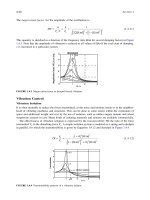
Typically, plastic strain is viewed as permanent strain. As illustrated in Figure 19.1,
in a uniaxial tensile specimen, the stress,

S

11

, can be increased to the point A, and
then unloaded along the path AB. The slope of the unloading portion is E, the same
as that of the initial elastic portion. When the stress becomes equal to zero, there
still is a residual strain,

E

i

, which is identified as the inelastic strain. However, if
instead the stress was increased to point C, it would encounter reversed loading at
point D, which reflects the fact that the elastic region need not include the zero-
stress value.

19.1.2 P

LASTICITY

We will present a constitutive equation for plasticity to illustrate how the tangent
modulus is stated. The ideas leading to the equation will be presented subsequently
in the section on thermoplasticity. With χχ
χχ

e




=



ITEN

22(

D

e

) and

D

e

denoting the
19
DD D=+
ri
,
∃= ∃ = ∃ =
∫∫∫
DD Ddt dt dt
rr ii
.
˙

.EE E== =
∫∫
FDF FDF FDF
TT
r
T
i

ri
dt dt

0749_Frame_C19 Page 243 Wednesday, February 19, 2003 5:34 PM
© 2003 by CRC CRC Press LLC

244

Finite Element Analysis: Thermomechanics of Solids

tangent-modulus tensor relating the elastic-strain rate to the stress rate (assuming
a linear relation), the constitutive equation of interest is
(19.4)
In Equation 19.4, ΨΨ
ΨΨ

i

is the yield function. ΨΨ
ΨΨ

i




=

0 determines a closed convex
surface in stress space called the yield surface. (We will see later that ΨΨ
ΨΨ

i

also serves
as a [complementary] dissipation potential.) The stress point remains on the yield
surface during plastic flow, and is moving toward its exterior. The plastic strain rate,
expressed as a vector, is typically assumed to be normal to the yield surface at the
stress point. If the stress point is interior to, or moving tangentially on, the yield
surface, only elastic deformation occurs. On all interior paths, for example, due to
unloading, the response is only elastic. Plastic deformation induces “hardening,”
corresponding to a nonvanishing value of

C

i

.



Finally,


k

is a history-parameter vector,
introduced to represent dependence on the history of plastic strain, for example,
through the amount of plastic work.
The yield surface is distorted and moved by plastic strain. In Figure 19.2(a), the
conventional model of isotropic hardening is illustrated in which the yield surface
expands as a result of plastic deformation. This model is unrealistic in predicting a
growing elastic region. Reversed plastic loading is encountered at much higher
stresses than isotropic hardening predicts. An alternative is kinematic hardening (see
Figure 19.2[b]), in which the yield surface moves with the stress point. Within a few
percentage points of plastic strain, the yield surface may cease to encircle the origin.

FIGURE 19.1

Illustration of inelastic strain.
S
11
E
11
A
C
E
E
E
F
E
i
B
D

˙˙˙ ˙
,
˙
˙
.
eCseCsC K
C
eii e ee i
i
ii i
i
ii
HH
== ==
=
∂
∂






∂
∂
=−
∂
∂
+
∂

∂






∂
∂














−
, ,
,
χχ
ΨΨΨΨΨΨΨΨΨΨ
1
k

ss ek
K
s
TT
e

0749_Frame_C19 Page 244 Wednesday, February 19, 2003 5:34 PM

Inelastic and Thermoinelastic Materials

245

A reference point interior to the yield surface, sometimes called the back stress,
must be identified to serve as the point at which the elastic strain vanishes. Com-
bined isotropic and kinematic hardening are shown in Figure 19.2(c). However, the
yield surface contracts, which is closer to actual observations (e.g., Ellyin [1997]).

FIGURE 19.2(a)

Illustration of yield-surface expansion under isotropic hardening.

FIGURE 19.2(b)

Illustration of yield-surface motion under kinematic hardening.
S
ll
S
l
S
lll

principal stresses S
l
S
ll
S
lll
path of stress point
S
lll
S
ll
S
l
path of stress point

0749_Frame_C19 Page 245 Wednesday, February 19, 2003 5:34 PM

246

Finite Element Analysis: Thermomechanics of Solids

The rate of movement must exceed the rate of contraction for the material to remain
stable with a positive tangent modulus.
Combining the elastic and inelastic portions furnishes the tangent-modulus tensor:
(19.5)
Suppose that in uniaxial tension, the elastic modulus is E

e

and the inelastic

modulus-relating stress and inelastic strain increments are E

i

,



and E

i

<< E

e

. The total
uniaxial modulus is then

19.2 THERMOPLASTICITY

As in Chapter 18, two potential functions are introduced to provide a systematic
way to describe irreversible and dissipative effects. The first is interpreted as the
Helmholtz free-energy density, and the second is for dissipative effects. To accom-
modate kinematic hardening, we also assume an extension of the Green and Naghdi
(G-N) (1965) formulation, in which the Helmholtz free energy decomposes into
reversible and irreversible parts, with the irreversible part depending on the “plastic
strain.” Here, it also depends on the temperature and a workless

internal state variable


.

19.2.1 B

ALANCE



OF

E

NERGY

The conventional equation for energy balance is augmented using a vector-valued, work-
less internal variable, αα
αα

0

, regarded as representing “microstructural rearrangements”:
(19.6)

FIGURE 19.2(c)

Illustration of combined kinematic and isotropic hardening.
S
lll
S

ll
S
l
path of stress point
χχχχχχχχ=+
[]
=+
−
−
−
ei eie
1
1
1
CC[].I
E
EE
i
ie
(/)
.
1 +
ρρ
ori o
h
˙
˙˙
˙
,
χ

00000
=+−∇++se e
TT T T
qs ββαα

0749_Frame_C19 Page 246 Wednesday, February 19, 2003 5:34 PM

Inelastic and Thermoinelastic Materials

247

where

χ

o

is the internal energy per unit mass in the undeformed configuration and

s



=



VEC

(


S

),

e



=



VEC

(

E

), and ββ
ββ

0

is the flux per unit mass associated with αα
αα

0

. However,

note that ββ
ββ



=



0

, thus ββ
ββ

i



=



−ββ
ββ

r

. Also,

c


is the internal energy per unit mass,

q

0

is the
heat-flux vector referred to undeformed coordinates, and

h

is the heat input per unit
mass, for simplicity’s sake, assumed independent of temperature. The state variables
are

E

r

,

E

i

, T, and αα
αα

0


.
The next few paragraphs will go over some of the same ground as for damped
elastomers in Chapter 18, except for two major points. In that chapter, the stress
was assumed to decompose into reversible and irreversible portions in the spirit of
elementary Voigt models. In the current context, the strain shows the decomposition
in the spirit of the classical Maxwell model. In addition, as seen in the following,
it proves beneficial to introduce a workless internal variable to give the model the
flexibility to accommodate phenomena such as kinematic hardening.
The Helmholtz free energy,

φ

, per unit mass and the entropy,

η

, per unit mass
are introduced using
(19.7)
Now,
(19.8)

19.2.2 E

NTROPY

-P

RODUCTION


I

NEQUALITY

The entropy now satisfies
(19.9)
Viewing

φ

r

as a differentiable function of

e

r

, T, and αα
αα

0

, we conclude that
(19.10)
Extending the G-N formulation, let

s


*

T



=



ρ

0

∂

φ

i

/

∂

e

i

and assume that


η

i



=



−∂

φ

i

/

∂

T
and

ρ

0

∂

φ


i

/

∂αα
αα

0



=

. Now,
(19.11)
The entropy-production inequality (see Equation 19.9) is now restated as
(19.12)
φ
=−
χη
T.
∇
00 0 0 0
TT
q −= +− − −+
ρρηρηρφ
000
TTh
T

r
T
i
ss
˙˙
˙
˙
˙
˙
.ee ββαα
ρη ρ
ρφ ρ η ρη
00000
000000
TT/T
TTT/T
˙
˙
˙˙
˙
˙
˙
.
≥− + +
≥−−+ + + −
∇∇
∇
TT
T
ri

hqq
q
TT
se se
T
ββαα
∂∂ ∂∂ ∂∂
φφρηφ
rr
T
rrrr
T
// /.es==− = T
000
ααββ
ββ
0i
T
se*
T
ii i i i i
T
==− =
ρφ η φ ρφ
0000
∂∂ ∂∂ ∂∂///. T ααββ
()
˙
.sse
TT

i
*−− ≥q
T
00
0∇ T/T
0749_Frame_C19 Page 247 Wednesday, February 19, 2003 5:34 PM
248 Finite Element Analysis: Thermomechanics of Solids
The inequality shown in Equation 19.12 can be satisfied if
(19.13)
The first inequality involves a quantity, s* = VEC(S*), with dimensions of stress.
In the subsequent sections, s* will be viewed as a reference stress, often called the
back stress, which is interior to a yield surface and can be used to characterize the
motion of the yield surface in stress space. In classical kinematic hardening in which
the hyperspherical yield surface does not change size or shape but just moves, the
reference stress is simply the geometric center. If kinematic hardening occurs, as
stated before, the yield surface need not include the origin even with small amounts
of plastic deformation. Thus, there is no reason to regard as vanishing at the
origin. Instead, = 0 is now associated with a moving-reference stress interior to
the yield surface, identified here as the back stress s*.
19.2.3 DISSIPATION POTENTIAL
As in Chapter 18, we introduce a specific dissipation potential, Ψ
i
, for which
(19.14a)
from which, with Λ
i
> 0 and Λ
t
> 0,
(19.14b)

On the expectation that properties governing heat transfer are not affected by
strain, we introduce the decomposition into inelastic and thermal portions:
(19.15a)
where Ψ
i
represents mechanical effects and is identified in the subsequent sections.
The thermal constitutive relation derived from the dissipation potential implies
Fourier’s law:
(19.15b)
The inelastic portion is discussed in the following section.
()
˙
sse
TT
i
*−≥ −∇≥00
00
(a) T/T (b).q
T
˙
e
r
˙
e
r
˙
/ /ess
ii
i
T

it
*=∋−∇=∂ ∋=−
ρρ
0000
ΛΛ (i) T / T (ii) (iii),∂∂ ∂ΨΨ
T
q
ρρ
000
0ΛΛ
it
(/ (/ ) .∂∂ ∂ >Ψ∋)∋+ ∂Ψ
0
qq
ΨΨΨ Ψ=+ =
it t
t

ρ
000
2
Λ
qq
T
,
−∇ =
00
T/T q /.Λ
t
0749_Frame_C19 Page 248 Wednesday, February 19, 2003 5:34 PM

Inelastic and Thermoinelastic Materials 249
19.3 THERMOINELASTIC TANGENT-MODULUS
TENSOR
The elastic strain rate satisfies a thermohypoelastic constitutive relation:
(19.16)
C
r
is a 9 × 9 second-order, elastic compliance tensor, and a
r
is the 9 × 1
thermoelastic expansion vector, with both presumed to be known from measure-
ments. Analogously, for rate-independent thermoplasticity, we seek tensors C
i
and
a
i
, depending on , e
i
, and T such that
(19.17a)
(19.17b)
During thermoplastic deformation, the stress and temperature satisfy a thermo-
plastic yield condition of the form
(19.18)
and Π
i
is called the yield function. Here, the vector k is introduced to represent the
effect of the history of inelastic strain, , such as work hardening. It is assumed to
be given by a relation of the form
(19.19)

The “consistency condition” requires that = 0 during thermoplastic flow, from
which
(19.20)
We introduce a thermoplastic extension of the conventional associated flow rule,
whereby the inelastic strain-rate vector is normal to the yield surface at the current
stress point,
(19.21)
˙
()
˙
.ess
rr r
*=−+
•
CTa
∋
˙
()
˙
eCss
ii i
*=−+
•
a T
˙
[]()()
˙
ess=+ − ++
•
CC

ri ri
* aaT.
Π
ii i
(, , , , ) ,∋=e k T
η
2
0
˙
e
i
˙
(,,)
˙
.kK k= ee
ii
T
˙
Π
i
d
d
d
d
d
d
d
d
d
d

ii
i
i
ii i
i
ΠΠ ΠΠΠ
∋
∋
˙
˙
˙
˙
˙
.++++ =
e
e
k
k
T
T
i
η
η
0
˙
˙
e
ii
i
T

i
i
d
d
d
d
=






=Λ
Π
Λ
Π
∋
(a) (b).
i
i
η
η
0749_Frame_C19 Page 249 Wednesday, February 19, 2003 5:34 PM
250 Finite Element Analysis: Thermomechanics of Solids
Equation 19.14a suggests that the yield function may be identified as the dissi-
pation potential: Π
i
=
ρ

0
Ψ
i
. Standard manipulation furnishes
(19.22)
and H must be positive for Λ
i
to be positive. Note that, in the current formulation,
the dependence of the yield function on temperature accounts for c
i
. The thermody-
namic inequality shown in Equation 19.13a is now satisfied if H > 0.
Next, note that s* depends on e
i
, T, and αα
αα
0
since s*
T
=
ρ
0
∂
φ
i
/∂e
i
. For simplicity’s
sake, we neglect dependence on αα
αα

0
and assume that a relation of the following form
can be measured for s*:
(19.23)
From Equations 19.16 and 19.17, the thermoinelastic tangent-modulus tensor
and thermal thermomechanical vector are obtained as
(19.24a)
(19.24b)
If appropriate, the foregoing formulation can be augmented to accommodate
plastic incompressibility.
19.3.1 EXAMPLE
We now provide a simple example using the Helmholtz free-energy density function
and the dissipation-potential function to derive constitutive relations. The following
expression involves a Von Mises yield function, linear kinematic hardening, linear
work hardening, and linear thermal softening.
˙
˙
˙
˙
˙
˙
e
ii i i i
T
i
i
ii
ii
i
T

i
i
ii
i
i
HH
T
HH
=∋+ = ∋+
=
∂
∂∋






∂
∂∋
==
∂
∂∋






∂

∂
=
∂
∂






=−
∂
∂
+
∂
∂






∂
C T c T

T
c
ab
ab
ek

K
T
η
2
2
C
ΨΨ ΨΨ
ΨΨΨ
ΨΨΨΨ
i
T
i
i
i
∂∋






+
∂
∂
∂
∂









η
2
T
˙˙
˙
/se
ee
e*
i
ii
T
T
ii
=+ =






=∂ ∂ ∂ΓΓΓΓ
ϑϑ
T T.
I
∂
∂

∂
∂
ΨΨ
2
˙˙
˙
es=+C aT
CCCII C C
CC CCI C
=+ −+
=++ + − + +
−
−
()[()]
[()()()]
ri i i
ri r ii r i i
ΓΓΓΓ
ΓΓΓΓ
1
1
aaa a
ϑ
0749_Frame_C19 Page 250 Wednesday, February 19, 2003 5:34 PM
Inelastic and Thermoinelastic Materials 251
i. Helmholtz free-energy density:
(19.25)
in which is a known constant. From Equation 19.28,
(19.26)
Finally,

(19.27)
ii. Dissipation potential:
(19.28)
(19.29)
Straightforward manipulations serve to derive
(19.30)
(19.31)
Consider a two-stage thermomechanical loading, as illustrated schematically in
Figure 19.3. Let S
I
, S
II
, S
III
denote the principal values of the 2
nd
Piola-Kirchhoff
stress, and suppose that S
III
= 0. In the first stage, with the temperature held fixed
at T
0
, the stresses are applied proportionally well into the plastic range. The center
of the yield surface moves along a line in the (S
1
, S
2
) plane, and the yield surface
expands as it moves. In the second stage, suppose that the stresses S
1

and

S
2
are
fixed, but that the temperature increases to T
1
and then to T
2
and T
3
. The plastic
strain must increase, thus, the center of the yield surface moves. In addition, strain
hardening tends to cause the yield surface to expand, while the increased temperature
tends to make it contract. However, in this case, thermal softening must dominate
strain hardening, and contraction must occur since the center of the yield surface
must move further along the path shown even as the yield surface continues to “kiss”
the fixed stresses S
I
and S
II
.
φφφ φ
φ
=+ =
=−−+
′
−
−−
ri i ii

rrrr r r r
k
ln

T T c T (T / T )
ρ
ρρ
03
0
11
00 0
21
ee
CC
T
TT
aee e/() ( )
′
c
r
∋= ∂ ∂ = − −
−
ρφ
0
1
0
( / ) [ ( )].
rr rrr
ee
T

C a TT
cT
T
c
r
r
=−
∂
∂
=
′
2
2
φ
ΨΨΨ Ψ=+ =
it t
t
T

ρ
000
2
Λ
qq
Ψ
i
T
i
kkkk k=∋∋− + − − = =∋
T

[ ( )]
˙
˙
01 2 0
0TT e
Hk kk kkk=∋∋= +− −
110120
T
[()]TT
Cab
T
T
T
iiii
HkH
k
H=
∋∋
∋∋
===
∋
∋∋
c
2
2
2

0749_Frame_C19 Page 251 Wednesday, February 19, 2003 5:34 PM
252 Finite Element Analysis: Thermomechanics of Solids
Unfortunately, accurate finite-element computations in plasticity and thermo-

plasticity often require close attention to the location of the front of the yielded
zone. This front will occur within elements, essentially reducing the continuity order
of the fields (discontinuity in strain gradients). Special procedures have been devel-
oped in some codes to address this difficulty.
The shrinkage of the yield surface with temperature provides an element of
the explanation of the phenomenon of adiabatic shear banding, which is commonly
encountered in some materials during impact or metal forming. In rapid processes,
plastic work is mostly converted into heat and on into high temperatures. There
is not enough time for the heat to flow away from the spot experiencing high
deformation. However, the process is unstable while the stress level is maintained.
Namely, as the material gets hotter, the rate of plastic work accelerates, thanks to
the softening evident in Figure 19.3. The instability is manifested in small, peri-
odically spaced bands, in the center of which the material is melted and resolidified,
usually in a much more brittle form than before. These bands can nucleate brittle
failure.
19.4 TANGENT-MODULUS TENSOR
IN VISCOPLASTICITY
The thermodynamic discussion in the previous section applies to thermoinelastic
deformation, for which the first example given concerned quasi-static plasticity and
thermoplasticity. However, it is equally applicable when rate sensitivity is present, in
which case viscoplasticity and thermoviscoplasticity are attractive models. An example
FIGURE 19.3 Effect of load and temperature on yield surface.
S
lll
S
ll
S
l
T
0

T
0
T
0
T
0
T
0
T
0
T
1
T
2
T
3
T
4
0749_Frame_C19 Page 252 Wednesday, February 19, 2003 5:34 PM
Inelastic and Thermoinelastic Materials 253
of a constitutive model, for example, following Perzyna (1971), is given in undeformed
coordinates as
(19.32)
and Ψ
i
(∋, e
i
, k, T,
η
i

) is a loading surface function. The elastic response is still
considered linear in the form
(19.33)
Recall from thermoplasticity that
(19.34)
Corresponding to , there is a reference stress s′ and a corresponding vector ′ =
s′ − s* such that Ψ
i
( ′, e
i
, k, T,
η
i
) = k(e
i
, k, T,
η
i
) determines a quasi-static, reference-
yield surface. The vectors and ′ have the same origin and direction, but the latter
terminates at the reference surface, while the latter terminates outside the reference
surface if inelastic flow is occurring. Interior to the surface, no inelastic flow occurs.
If exterior to the surface, inelastic flow occurs at a rate dependent on the distance to
the exterior of the reference surface. This situation is illustrated in Figure 19.4.
FIGURE 19.4 Illustration of reference surface in viscoplasticity.
µ
ω

=< − >













<− >=
−−≥





∂
∂∋
∂
∂∋
∂
∂∋
˙
,e
i
T
T
kk

kk
11
110
ΨΨ
ΨΨ
Ψ
ΨΨ
i
i
ii

, if
0, otherwise,
i
ii
˙˙
˙
es
rr r
=+
−
χχαα
1
T.
˙˙
˙
.se
ee
e*
i

ii
T
i
T
ii
=+ =






=∂ΓΓΓΓ
ϑϑ
TT
∂
∂
∂
∂
Ψ∂Ψ/∂
2
∋
∋
∋
∋
∋
S
lll
S
ll

S
l
S
∗
stress point
0749_Frame_C19 Page 253 Wednesday, February 19, 2003 5:34 PM
254 Finite Element Analysis: Thermomechanics of Solids
It should be evident that viscoplasticity and thermoviscoplasticity can be for-
mulated to accommodate phenomena such as kinematic hardening and thermal
shrinkage of the reference-yield surface.
The tangent-modulus matrix now reduces to elastic relations, and viscoplastic
effects can be treated as an initial force (after canceling the variation) since
(19.35)
In particular, the Incremental Principle of Virtual Work is now stated, to first order, as
(19.36)
19.5 CONTINUUM DAMAGE MECHANICS
Ductile fracture occurs by processes associated with the notion of damage. An
internal-damage variable is introduced that accumulates with plastic deformation.
It also manifests itself in reductions in properties, such as the experimental values
of the elastic modulus and yield stress. When the damage level in a given element
reaches a known or assumed critical value, the element is considered to have failed.
It is then removed from the mesh (considered to be no longer supporting the load).
The displacement and temperature fields are recalculated to reflect the element
deletion.
There are two different schools of thought on the suitable notion of a damage
parameter. One, associated with Gurson (1977), Tvergaard (1981), and Thomasson
(1990), considers damage to occur by a specific mechanism occurring in a three-
stage process: nucleation of voids, their subsequent growth, and their coalescence
to form a macroscopic defect. The coalescence event is used as a criterion for element
failure. The parameter used to measure damage is the void-volume fraction f. Models

and criteria for the three processes have been formulated. For both nucleation and
growth, evolution of f is governed by a constitutive equation of the form
(19.37)
⋅= + − −






<− >












∂
∂∋
∂
∂∋
∂
∂∋
˙˙

˙
.seχχχχααΓΓ
χχ
ΨΨ
rrr
r
v
T
T
k
T
i
i
ii
µ
1
Ψ
ΨΨ
δδ δρ
δδ
µ
∆∆ ∆ ∆ ∆ ∆
∆∆ ∆
ee e uu
ue
T
ro
T
rr o
T

oo
T
o
T
r
v
T
T
o
dV dV dV
dS
k
dV
i
∫∫ ∫
∫∫
++
+−






<− >













∂
∂∋
∂
∂∋
∂
∂∋
χχχχαα
ττΓΓ
χχ
T
=
i
ii
˙˙
1
Ψ
Ψ
ΨΨ
˙
(, ,),ffT
i
=ΞΞ e
0749_Frame_C19 Page 254 Wednesday, February 19, 2003 5:34 PM

Inelastic and Thermoinelastic Materials 255
for which several specific forms have been proposed. To this point, a nominal stress
is used in the sense that the reduced ability of material to support stress is not
accommodated.
The second school of thought is more empirical in nature and is not dependent
on a specific mechanism. It uses the parameter D, which is interpreted as the fraction
of damaged area A
d
to total area A
o
that the stress (traction) acts on. Consider a uniaxial
tensile specimen with damage, but experiencing elastic behavior. Suppose that dam-
aged area A
d
can no longer support a load (is damaged). For a given load P, the true
stress at a point in the undamaged zone is Here, S′
is a nominal stress, but is also the measured stress. If E is the elastic modulus
measured in an undamaged specimen, the modulus measured in the current specimen
will be E′ = E(1 − D), demonstrating that damage is manifest in small changes in
properties.
As an illustration of damage, suppose specimens are loaded into the plastic
range, unloaded, and then loaded again. Without damage, the stress-strain curve
should return to its original path. However, due to the damage, there are slight
changes in the elastic slope, in the yield stress, and in the slope after yield (exag-
gerated in Figure 19.5).
From the standpoint of thermodynamics, damage is a dissipative internal variable.
In reality, the amount of mechanical or thermal energy absorbed by damage is probably
small, so that its role in the energy-balance equation can be neglected. At the risk of
being slightly conservative, in dynamic (adiabatic) problems, the plastic work can be
assumed to be completely converted into heat. Even so, for the sake of a consistent

framework for treating dissipation, a dissipation potential, ΨΨ
ΨΨ
d
, can be introduced for
damage, as has been done, for example, by Bonora (1997). The contribution to the
irreversible entropy production can be introduced in the form ≥ 0, in which
is the “force” associated with flux . Positive dissipation is assured if we assume
(19.38)
FIGURE 19.5 Illustration of effect of damage on elastic-plastic properties.
S
11
E
11
S
y1
S
y2
E
p1
E
p2
E
1
E
2
S
y3
E
p3
E

3
SS
DD
===′
−− −
P
AA
1
1
P
A
1
1
oD o
.
D
˙
D D
˙
D
D =
∂
∂
=>
Ψ
Ψ
d
d
i
d

i
D
D
˙
(
˙
,(, , T, ) ,T, ) 0.
d
1
2
2
ΛΛeekk
0749_Frame_C19 Page 255 Wednesday, February 19, 2003 5:34 PM
256 Finite Element Analysis: Thermomechanics of Solids
An example of a satisfactory function is Λ
d
(e
i
, T, k) = Λ
do
∫(s − s*) dt, Λ
do
a
positive constant, showing damage to depend on plastic work.
Specific examples of constitutive relations for damage are given, for example,
in Bonora (1997).
At the current values of the damage parameter, the finite-element equations are
solved for the nodal displacements, from which the inelastic strains can be computed.
This information can then be used to update the damage-parameter values. Upon
doing so, the damage-parameter values are compared to critical values. As stated

previously, if the critical value is obtained, the element is deleted. The path of deleted
elements can be viewed as a crack.
The code LS-DYNA Ver. 9.5, (2000) incorporates a material model that includes
viscoplasticity and damage mechanics. It can easily be upgraded to include thermal
effects, assuming that all viscoplastic work is turned into heat. Such a model has
been shown to reproduce the location and path of a crack in a dynamically loaded
welded structure (see Moraes [2002]).
19.6 EXERCISES
1. In isothermal plasticity, assuming the following yield function, find the
uniaxial stress-strain curve:
Assume small strain and that the plastic strain is incompressible: tr(E
i
) = 0.
2. Regard the expression in Exercise 1 as defining the reference-yield surface
in viscoplasticity, with viscosity h
v
.

Find the stress-strain curve under
uniaxial tension if a constant strain rate is imposed.
˙
e
i
Ψ
i

0
.=− − −+







∫
()()
˙˙
sese eekkkk dt
i
T
io i
T
i
t
11 2
0749_Frame_C19 Page 256 Wednesday, February 19, 2003 5:34 PM
© 2003 by CRC CRC Press LLC © 2003 by CRC CRC Press LLC