Finite Element Analysis - Thermomechanics of Solids Part 17 potx
Bạn đang xem bản rút gọn của tài liệu. Xem và tải ngay bản đầy đủ của tài liệu tại đây (680.33 KB, 12 trang )
215
Incremental Principle
of Virtual Work
17.1 INCREMENTAL KINEMATICS
Recall that the displacement vector
u
(
X
) is assumed to admit a satisfactory approx-
imation at the element level in the form
u
(
X
)
=
ϕϕ
ϕϕ
T
(
X
)ΦΦ
ΦΦ
γγ
γγ
(
t
). Also recall that the
deformation-gradient tensor is given by
F
=
Suppose that the body under study
is subjected to a load vector,
P
, which is applied incrementally via load increments,
∆
j
P
. The load at the
n
th
load step is denoted as
P
n
. The solution,
P
n
, is known, and
the solution of the increments of the displacements is sought. Let
∆
n
u
=
u
n
+
1
−
u
n
,
so that
∆
n
u
=
ϕϕ
ϕϕ
T
(
X
)ΦΦ
ΦΦ
∆
n
γγ
γγ
. By suitably arranging the derivatives of
∆
n
u
with respect
to
X
, a matrix,
M
(
X
), can easily be determined for which
VEC
(
∆
n
F
)
=
M
(
X
)
∆
n
γγ
γγ
.
We next consider the Lagrangian strain,
E
(
X
)
=
(
F
T
F
−
I
). Using Kronecker
Product algebra from Chapter 2, we readily find that, to first order in increments,
(17.1)
This form shows the advantages of Kronecker Product notation. Namely, it
enables moving the incremental displacement vector to the end of the expression
outside of domain integrals, which we will encounter subsequently.
Alternatively, for the current configuration, a suitable strain measure is the
Eulerian strain,
«
=
(
I
−
F
−
T
F
−−
−−
1
), which refers to deformed coordinates. Note that
since
∆
n
(
FF
−−
−−
1
)
=
0
,
∆
n
F
−−
−−
1
=
−
F
−−
−−
1
∆
n
FF
−−
−−
1
. Similarly,
∆
n
F
−−
−−
T
=
−
F
−
T
∆
n
F
T
F
−
T
. Simple
manipulation furnishes that
(17.2)
There also are geometric changes for which an incremental representation is
useful. For example, since the Jacobian
J
=
det(
F
) satisfies
dJ
=
Jtr
(
F
−
1
d
F
), we obtain
17
∂
∂
x
x
.
1
2
∆∆
∆∆
∆
∆∆
nn
nn
T
n
nn
VEC
VEC
VEC
e
GG
T
TT
TTT
=
=+
=⊗+⊗
==⊗+⊗
()
[]
[]()
,[ ]()
E
M
1
2
1
2
1
2
FF FF
IF F IU F
gIFFIUXg .
1
2
VEC
n
TT
n
() [ ] .∆∆=⊗+⊗
−− − − −−
1
2
11
FF FUF FF Mg
T1
«
0749_Frame_C17 Page 215 Wednesday, February 19, 2003 5:24 PM
© 2003 by CRC CRC Press LLC
216
Finite Element Analysis: Thermomechanics of Solids
the approximate formula
(17.3)
Also of interest are
(17.4)
Using Equation 17.4, we obtain the incremental forms
(17.5)
17.2 INCREMENTAL STRESSES
For the purposes of deriving an incremental variational principle, we shall see that
the incremental 1
st
Piola-Kirchhoff stress, , is the starting point. However, to
formulate mechanical properties, the objective increment of the Cauchy stress,
is the starting point. Furthermore, in the resulting variational statement, which we
called the
Incremental Principle of Virtual Work
, we find that the quantity that
appears is the increment of the 2
nd
Piola-Kirchhoff stress,
∆
n
S
.
From Chapter 5, we learned that
, from which, to first order,
(17.6)
For the Cauchy stress, the increment must take into account the rotation of the
underlying coordinate system and thereby be objective. We recall the objective
Truesdell stress flux, , introduced in Chapter 5:
(17.7)
∆∆
∆
∆
J Jtr
JVEC VEC
VEC J
n
n
T
n
T
=
=
=
−
−
−
()
() ()
()
FF
FF
F
1
1T
T
M γγ.
ddS
dt
tr dS
d
dt
d
dt
dS tr dS
T
TT
T
[]
[() ]
[( ) ]
[() ]
n
Dn
n
nDn n
D
=−
=−
=−
IL
IL
nDn
∆∆∆∆γγ
γγ
γγ
n
TT T T
n
n
TT T T T
n
n
TT TT T
n
dS dS VEC
dS dS VEC
[] [ () ]
[( ) ]
[()()].
nnFnFU
nnnF n n FU
nFnnFn
=−⊗
=⊗−⊗
=−⊗
−−
−−
−−
M
M
M
∆∆
∆∆
∆
n
S
∆
o
n
T,
SS= F
T
∆∆ ∆
nn
T
n
T
SSS=+FF.
∂∂T
o
/
t
∂∂=∂∂+ − −TTT T
o
//() .tttr
T
DL LT
0749_Frame_C17 Page 216 Wednesday, February 19, 2003 5:24 PM
© 2003 by CRC CRC Press LLC
Incremental Principle of Virtual Work
217
Among the possible stress fluxes, it is unique in that it is proportional to the
rate of the 2
nd
Piola-Kirchhoff stress, namely
(17.8)
An objective Truesdell stress increment is readily obtained as
(17.9)
Furthermore, once has been determined, the (nonobjective) incre-
ment of the Cauchy stress can be computed using
(17.10)
from which
(17.11)
17.3 INCREMENTAL EQUILIBRIUM EQUATION
We now express the incremental equation of nonlinear solid mechanics (assuming
that there is no net rigid-body motion). In the deformed (Eulerian) configuration,
equilibrium at
t
n
requires
(17.12)
Referred to the undeformed (Lagrangian) configuration, this equation becomes
(17.13)
in which, as indicated before, is the 1
st
Piola-Kirchhoff stress,
S
denotes the surface
(boundary) in the deformed configuration, and
n
0
is the surface normal vector in the
undeformed configuration. Suppose the solution for is known as at time
t
n
and
is sought at
t
n
+
1
. We introduce the increment to denote A similar
definition is introduced for the increment of the displacements. Now, equilibrium
applied to and implies
(17.14)
∂∂ ∂ ∂ST//.tJ t
T
=
−−
FF
1
o
VEC VEC
n
T
n
J
() ().∆∆
o
TS=⊗
1
FF
VEC
()
∆
o
n
T
∆∆ ∆ ∆ ∆
o
n
nnn
T
n
T
trTTT TT=+ − −
−−−
() ,FF FF F F
11
VEC VEC VEC
n
n
TT T T
n
( ) ( ) [ ( ) ( ) ( )] .∆∆ ∆TTT T TM=+ −⊗−⊗
−− −
o
FFIIF γγ
T
T
dS dVnu
∫∫
=
ρ
˙˙
.
S
T
dS dVnu
00 0 0
∫∫
=
ρ
˙˙
,
S
S S
n
∆
n
S
SS
nn+
−
1
.
S
n+1
S
n
∆∆
n
T
n
dS dVS nu
00
0
0
∫∫
=
ρ
˙˙
.
0749_Frame_C17 Page 217 Wednesday, February 19, 2003 5:24 PM
© 2003 by CRC CRC Press LLC
218
Finite Element Analysis: Thermomechanics of Solids
Application of the divergence theorem furnishes the differential equation
(17.15)
17.4 INCREMENTAL PRINCIPLE OF VIRTUAL WORK
To derive a variational principle for the current formulation, the quantity to be varied is
the incremental displacement vector since it is now the unknown. Following Chapter 5,
Equation 17.15 is multiplied by (
δ
∆
n
u
)
T
.
Integration is performed over the domain.
The Gauss divergence theorem is invoked once.
Terms appearing on the boundary are identified as primary and secondary
variables.
Boundary conditions and constraints are applied.
The reasoning process is similar to that in the derivation of the Principle of
Virtual Work in finite deformation in which
u
is the unknown, and furnishes
(17.16)
in which ττ
ττ
0
is the traction experienced by
dS
0
. The fourth term describes the virtual
external work of the incremental tractions. The first term describes the virtual internal
work of the incremental stresses. The third term describes the virtual internal work
of the incremental inertial forces. The second term has no counterpart in the previ-
ously formulated Principle of Virtual Work in Chapter 5, and arises because of
geometric nonlinearity. We simply call it the geometric stiffness integral. Due to the
importance of this relation, Equation 17.16 is derived in detail in the equations that
follow. It is convenient to perform the derivation using tensor-indicial notation:
(17.17)
The first term on the right is converted using the divergence theorem to
(17.18)
which is recognized as the fourth term in Equation 17.16.
∇
T
∆∆
n
T
n
T
S =
ρ
0
˙˙
.u
tr dV dV dV dS
nn nn n
T
nn
T
n
()
˙˙
,
δδδρδ
∆∆ ∆∆ ∆ ∆ ∆∆ES S
TT
FF u u u
00
0
0
0
0
∫∫∫∫
++ =ττ
δδδ
δρ
∆∆ ∆∆ ∆∆
∆∆
ni
j
nij
j
ni nij
j
ni nij
ni ni
u
X
SdV
X
uSdV
X
uSdV
uudV
∂
∂
∂
∂
∂
∂
() [ ()] [ ]
˙˙
.
000
00
∫∫ ∫
∫
=−
=
∂
∂X
u S dV u n S dS
udS
ni nij ni j nij
ni j
j
[()] ( )
δδ
δτ
∆∆ ∆ ∆
∆
00
00
∫∫
∫
=
=
0749_Frame_C17 Page 218 Wednesday, February 19, 2003 5:24 PM
© 2003 by CRC CRC Press LLC
Incremental Principle of Virtual Work
219
To first-order in increments, the second term on the right is written, using tensor
notation, as
(17.19)
The second term is recognized as the second term in Equation 17.16.
The first term now becomes
(17.20)
which is recognized as the first term in Equation 17.16.
17.5 INCREMENTAL FINITE-ELEMENT EQUATION
For present purposes, let us suppose constitutive relations in the form
(17.21)
in which D(X,
γ
) is the fourth-order tangent modulus tensor. It is rewritten as
(17.22)
Also for present purposes, we assume that ∆ττ
ττ
0
is prescribed on the boundary S
0
, a
common but frequently unrealistic assumption that is addressed in a subsequent section.
In VEC notation, and using the interpolation models, Equation 17.16 becomes
(17.23)
∂
∂X
u S dV tr dV
tr dV
tr dV tr dV
j
ni nij n n
nn
T
n
T
T
nn n n
T
[] ( )
([ ])
()()
δδ
δ
δδ
∆∆ ∆∆
∆∆ ∆
∆∆ ∆ ∆
00
0
00
∫∫
∫
∫∫
=
=+
=+
F
FF F
FF FF
S
SS
SS
tr dV tr dV
tr dV
T
nn
T
nn
T
n
n
T
n
() [ ]
()
FF FF FF
δδδ
δ
∆∆ ∆ ∆ ∆
∆∆
SS
S
00
0
1
2
∫∫
∫
=+
=Ε
∆∆
nnn
SD E= (, ) ,X
γ
∆∆
nnn
sX=χχ(, )
γ
e
sSe D== =VEC VEC TEN22( ), ( ), ( ). E
χ
δ
∆∆∆∆
nTGn nn
γγγγγγ
T
KK M f[( )
˙˙
]++−=0
KM M KMSM
M
T
TT
G
T
TT
n
T
dV dV
dV dS
==⊗
==
∫∫
∫∫
GG
χχ
00
00 000
I
f
ρρ
ΦΦϕϕϕϕΦΦΦΦϕϕττ∆∆
0749_Frame_C17 Page 219 Wednesday, February 19, 2003 5:24 PM
© 2003 by CRC CRC Press LLC
220 Finite Element Analysis: Thermomechanics of Solids
K
T
is now called the tangent modulus matrix, K
G
is the geometric stiffness matrix,
M is the (incremental) mass matrix, and ∆
n
f is the incremental force vector.
17.6 INCREMENTAL CONTRIBUTIONS
FROM NONLINEAR BOUNDARY CONDITIONS
Again, let I
i
denote the principal invariants of C, and let i = VEC(I), c
2
= VEC(C
2
),
, and A
i
= ∂n
i
/∂c. Recall from Chapter 2 that
(17.24)
Equation 17.23 is complete if increments of tractions are prescribed on the
undeformed surface S
0
. We now consider the more complex situation in which
ττ
ττ
is
referred to the deformed surface S, on which they are prescribed functions of u.
From Chandrasekharaiah and Debnath (1994), conversion is obtained using
(17.25)
and from Nicholson and Lin (1997b)
(17.26)
Suppose that ∆ττ
ττ
is expressed on S as follows:
(17.27)
Here, is prescribed, while A
M
is a known function of u. Also, S
0
is the
undeformed counterpart of S. These relations are capable of modeling boundary
conditions, such as support by a nonlinear elastic foundation.
From the fact that ττ
ττ
dS = ττ
ττ
0
dS
0
=
µ
ττ
ττ
0
dS, we conclude that ττ
ττ
=
µ
ττ
ττ
0
. It follows that
(17.28)
n
c
T
ii
I=∂ ∂/
nnc
AAI
121 32129
1293 19
==−=−+ =⊗
==− =⊗+⊗−++−
ii cc
ii
III
I
TTTT
ni III
0 A I C C I ic ci ii I()().
ττττdS dS dS dS
dS dS J
TT
TTT
==
===⊗
−
00 00 0
000003
nq nq
nC n n nn
1
µµ
∆∆
µµ µ
≈= ≈ =⊗ddmcmc m n nA
TT TTT
,/.
003
2
∆∆ ∆ττττ=−Au
M
T
.
dτ
τ
∆∆∆
∆∆ ∆
ττττ
ττ
ττ
ττ
0
2
2
1
1
=−
=− −
µµ
µ
µµ
()Am
M
TT
uc
0749_Frame_C17 Page 220 Wednesday, February 19, 2003 5:24 PM
© 2003 by CRC CRC Press LLC
Incremental Principle of Virtual Work 221
From the Incremental Principle of Virtual Work, the rhs term is written as
(17.29)
Recalling the interpolation models for the increments, we obtain an incremental
force vector plus two boundary contribution to the stiffness terms. In particular,
(17.30)
The first boundary contribution is from the nonlinear elastic foundation coupling
the traction and displacement increments on the boundary. The second arises from
geometric nonlinearity when the traction increment is prescribed on the current
configuration.
17.7 EFFECT OF VARIABLE CONTACT
In many, if not most, “real-world” problems, loads are transmitted to the member of
interest via contact with other members, for example, gear teeth. The extent of the
contact zone is an unknown to be determined as part of the solution process. Solution
of contact problems, introduced in Chapter 15, is a difficult problem that has absorbed
the attention of many investigators. Some algorithms are suited primarily for linear
kinematics. Here, a development is given for one particular formulation, which is
mostly of interest for explicitly addressing the effect of large deformation.
Figure 17.1 shows a contactor moving into contact with a foundation that is
assumed to be rigid. We seek to follow the development of the contact area and the
tractions arising throughout it. From Chapter 15, we recall that corresponding to a
point x on the contactor surface there is a target point y(x) on the foundation to
which the normal n(x) at x points. As the contactor starts to deform, n(x) rotates
and points toward a new value, y(x). As the point x approaches contact, the point
y(x) approaches the foundation point, which comes into contact with the contactor
point at x.
We define a gap function, g, using y(x) = x + gn. Let m be the surface normal-
vector to the target at y(x). Let S
c
be the candidate contact surface on the contactor,
whose undeformed counterpart is S
0c
. There also is a candidate contact surface S
f
on the foundation.
We limit our attention to bonded contact, in which particles coming into contact
with each other remain in contact. Algorithms for sliding contact with and without
friction are available. For simplicity’s sake, we also assume that shear tractions, in
δδ
µµ
∆∆ ∆ ∆ ∆ ∆uuAuc
TT
M
TT
dS dS
ττττ
ττ
00
2
0
1
∫∫
=−−
() .m
δδδ
∆∆ ∆∆ ∆ ∆u
TTT
BF BN
dSττγγγγγγ
00
∫
=− +fKK[]
∆∆f K NA N K m== =
∫∫ ∫
1
00 0
µµ
ττ
ττ
dS dS dS
BF M
TT
BN
2
T
,, G
0749_Frame_C17 Page 221 Wednesday, February 19, 2003 5:24 PM
© 2003 by CRC CRC Press LLC
222 Finite Element Analysis: Thermomechanics of Solids
the osculating plane of point of interest, are negligible. Suppose that the interface
can be represented by an elastic foundation satisfying the incremental relation
(17.31)
Here,
τ
n
= n
T
τ
and u
n
= n
T
u are the normal components of the traction and
displacement vectors. Since the only traction to consider is the normal traction (to
the contactor surface), the transverse components of ∆u are not needed (do not result
from work). Also, k(g) is a nonlinear stiffness function given in terms of the gap by,
for example,
(17.32)
As in Chapter 15, when g is positive, the gap is open and k approaches k
L
, which
should be chosen as a small number, theoretically zero. When g becomes negative,
the gap is closed and k approaches k
H
, which should be chosen as a large number,
theoretically infinity to prevent penetration of the rigid body).
Under the assumption that only the normal traction on the contactor surface is
important, it follows that
ττ
ττ
= t
n
n, from which
(17.33)
FIGURE 17.1 Contact.
foundation
y(x)
contactor
g
n
m
∆∆
τ
nn
kg u=− () .
kg
k
gkkk
H
k
rLHL
() ( ) , / .=− −
+>>
π
π
αε
2
1arctan
∆∆ ∆
ττ
=+
ττ
nn
nn.
0749_Frame_C17 Page 222 Wednesday, February 19, 2003 5:24 PM
© 2003 by CRC CRC Press LLC
Incremental Principle of Virtual Work 223
The contact model contributes the matrix K
c
to the stiffness matrix as follows
(see Nicholson and Lin, 1997b):
(17.34)
To update the gap, use the following relations proved in Nicholson and Lin (1997-b).
The differential vector, dy, is tangent to the foundation surface, hence, m
T
dy = 0. It
follows that
(17.35)
Using Equation 17.5, we may derive, with some effort, that
(17.36)
17.8 INTERPRETATION AS NEWTON ITERATION
The (nonincremental) Principle of Virtual Work can be restated in the undeformed
configuration as
(17.37)
We assume for convenience that
ττ
ττ
is prescribed on S
o
. The interpolation model
satisfies the form
(17.38)
δµ δτµ
δ
∆∆ ∆ ∆
∆∆
u
K
T
ττ
γγγγ
dS u dS
n
T
n
T
c
00
∫∫
=
=−
K Nn m Nnn N N h
cn
TT
cc
TT
cn
T
c
dS k g dS dS=− + +
∫∫ ∫
2
000
τµτµ
ββ () .
0 =+ +
=−
+
mu mnmn
mu mn
mn
TTT
TT
T
dgd dg
g
g
∆
∆∆
.
∆∆g
g
==−
+
=⊗−⊗
−−
ΓΓγγΓΓ
TT
TT
T
TTTTTTT
Nh
n
hnnF nnFM,,[[()]].
m
m
tr dV dV dS
o
T
o
T
o
()
˙˙
.
δδρδ
ES u u u
∫∫∫
+=ττ
( )
δδ
eBB
B I I I IU X
B I F F IU X
F
u
X
=+
[]
=⊗+⊗
=⊗+⊗
()
=
∂
∂
L
T
NL
T
L
T
NL
T
u
T
u
u
γγγγ
1
2
1
2
()()
()
.
M
M
0749_Frame_C17 Page 223 Wednesday, February 19, 2003 5:24 PM
© 2003 by CRC CRC Press LLC
224 Finite Element Analysis: Thermomechanics of Solids
Clearly, F
u
and B
NL
are linear in γγ
γγ
.
Upon cancellation of the variation d γγ
γγ
Τ
, an algebraic equation is obtained as
(17.39)
At the load step, Newton iteration is expressed as
(17.40)
or as a linear system
(17.41)
If the load increments are small enough, the starting iterate can be estimated as the
solution from the n
th
load step. Also, a stopping (convergence) criterion is needed
to determine when the effort to generate additional iterates is not rewarded by
increased accuracy.
Careful examination of the relations from this and the incremental formulations
uncovers that
(17.42)
so that the incremental stiffness matrix is the same as the Jacobian matrix in Newton
iteration. This, of course, is a satisfying result. The Jacobian matrix can be calculated
by conventional finite-element procedures at the element level followed by conven-
tional assembly procedures. If the incremental equation is only solved once at each
load increment, the solution can be viewed as the first iterate in a Newton iteration
scheme. The one-time incremental solution can potentially be improved by additional
iterations, as shown in Equation 17.41, but at the cost of computing the “residual”
Φ at each load step.
17.9 BUCKLING
Finite-element equations based on classical buckling equations for beams and plates
were addressed in Chapter 14. In the classical equations, geometrically nonlinear
terms appear through a linear correction term, thereby furnishing linear equations.
Here, in the absence of inertia and nonlinearity in the boundary conditions, we briefly
present a general viewpoint based on the incremental equilibrium equation
(17.43)
ΦΦγγγγττ(,) [( ( ]
˙˙
,.fBB)s ufN=+ + =
∫∫∫
LNL o
T
o
T
oo
dV dV dSN
ρ
γγγγΦΦγγ
ΦΦ
γγ
n
v)
n
)
n
)
nn
)
n
,
+
+
+
−
++ + +
−
=−
()
=
∂
∂
()
1
1
1
1
11 1 1
1
(( ( (
,,
νν ν
γ
Jf J f
JfγγγγΦΦγγ
γγγγγγγγ
n
v)
n
v
n
v
n
n
v)
n
v
n
(v )
n
v
+
+
+++
+
+
++
+
+
−
()
=
()
=+ −
[]
1
1
111
1
1
11
1
1
(() ()
(() ()
,,
.
JK K=+
TG
,
() .KK f
TGn n
+=
++
∆∆γγ
11
0749_Frame_C17 Page 224 Wednesday, February 19, 2003 5:24 PM
© 2003 by CRC CRC Press LLC
Incremental Principle of Virtual Work 225
This solution predicts a large incremental displacement if the stiffness matrix
K
T
+ K
G
is ill-conditioned or outright singular. Of course, in elastic media, K
T
is
positive-definite. However, in the presence of in-plane compression, K
G
may have
a negative eigenvalue whose magnitude is comparable to the smallest positive eigen-
value of K
T
. To see this recall that
(17.44)
We suppose that the element in question is thin in a local z (out-of-plane
direction). This suggests the assumption of plane stress. Now, in plate-and-shell
theory, it is necessary to add a transverse shear stress on the element boundaries to
allow the element to support transverse loads. We assume that the transverse shear
stresses only appear in the incremental force term and the tangent stiffness term,
and that the geometric stiffness term strictly satisfies the plane-stress assumption. It
follows that if the z-direction is out of the plane, in the geometric stiffness term,
(17.45)
In classical buckling, it is assumed that loads applied proportionately induce
proportionate in-plane stresses. Thus, for a given load path, only one parameter,
the length of the straight line the stress point traverses in the space of in-plane
stresses, arises in the eigenvalue problem for the critical buckling load. In nonlinear
problems, there is no assurance that the stress point follows a straight line. Instead,
if l denotes the distance along the line followed by the load point in proportional
loading, the stresses become numerical functions of l.
As a simple alternative to the general case, we consider buckling of a single
element and suppose that the stresses appearing in Equation 17.46 are applied in a
compressive sense along the faces of the element in a proportional manner whereby
(17.46)
in which the circumflex implies a reference value along the stress path at which l = 1,
and the negative signs on the stresses are present since buckling is associated with
compressive stresses. At the element level, the equation now becomes
(17.47)
KGG K I
T
TT
G
T
dV dV==⊗
∫∫
MM MMχ
00
S .
SI
III
III
III
⊗→
SS
SS
11 12
12 22
0
0
000
.
SI⊗→
−−
−−
λ
(
ˆ
)(
ˆ
)
(
ˆ
)(
ˆ
),
SS
SS
11 12
12 22
0
0
000
III
III
III
(
ˆ
).KK f
TGn n
−=
++
λ
∆∆γγ
11
0749_Frame_C17 Page 225 Wednesday, February 19, 2003 5:24 PM
© 2003 by CRC CRC Press LLC
226 Finite Element Analysis: Thermomechanics of Solids
At a given load increment, the critical buckling load for the current path, as a
function of two angles determining the path in the stress space illustrated in
Chapter 14, is obtained by computing the l value rendering singular.
17.10 EXERCISES
1. Assuming linear interpolation models for u,v in a plane triangular
membrane element with vertices (0,0),(1,0),(0,1), obtain the matrix M,
G, B
L
, and B
NL.
2. Repeat Exercise 1 with linear interpolation models for u, v, and w in a
tetrahedral element with vertices (0,0,0),(1,0,0),(0,1,0),(0,0,1).
(
ˆ
)KK
TG
−
λ
0749_Frame_C17 Page 226 Wednesday, February 19, 2003 5:24 PM
© 2003 by CRC CRC Press LLC