181

Torsion and Buckling

14.1 TORSION OF PRISMATIC BARS

Figure 14.1 illustrates a member experiencing torsion. The member in this case is
cylindrical with length

L

and radius

r

0

. The base is fixed, and a torque is applied at
the top surface, which causes the member to twist. The twist at height

z

is

θ

(z), and
at height

L

, it is

θ

0

.
Ordinarily, in the finite-element problems so far considered, the displacement is
the basic unknown. It is approximated by an interpolation model, from which an
approximation for the strain tensor is obtained. Then, an approximation for the stress
tensor is obtained using the stress-strain relations. The nodal displacements are
solved by an equilibrium principle, in the form of the Principle of Virtual Work. In
the current problem, an alternative path is followed in which stresses or, more
precisely, a stress potential, is the unknown. The strains are determined from the
stresses. However, for arbitrary stresses satisfying equilibrium, the strain field may
not be compatible. The compatibility condition (see Chapter 4) is enforced, furnishing

FIGURE 14.1

Twist of a prismatic rod.
14
section before twist
section after twist
z
T
θ
0
r
0

θ
φ
x
z
y
L
x

0749_Frame_C14 Page 181 Wednesday, February 19, 2003 5:41 PM
© 2003 by CRC CRC Press LLC

182

Finite Element Analysis: Thermomechanics of Solids

a partial differential equation known as the Poisson Equation. A variational argument
is applied to furnish a finite-element expression for the torsional constant of the
section.
For the member before twist, consider points

X

and

Y

at angle

φ


and at radial
position

r

. Clearly,

X



=



r

cos

φ

and

Y



=




r

sin

φ

. Twist induces a rotation through angle

θ

(

z

), but it does not affect the radial position. Now,

x



=



r

cos(

φ




+



θ

),

y



=



r

sin(

φ



+




θ

).
Use of double-angle formulae furnishes the displacements, and restriction to small
angles

θ

furnishes, to first order,
(14.1)
It is also assumed that torsion does not increase the length of the member, which
is attained by requiring that axial displacement

w

only depends on

X

and

Y

. The
quantity

w

(


X

,

Y

) is called the

warping function

.
It is readily verified that all strains vanish except

E

xz

and

E

yz

, for which
(14.2)
Equilibrium requires that
(14.3)
The equilibrium relation can be identically satisfied by a potential function


y

for which
(14.4)
We must satisfy the compatibility condition to ensure that the strain field arises
from a displacement field that is unique to within a rigid-body translation and
rotation. (Compatibility is automatically satisfied if the displacements are considered
the unknowns and are approximated by a continuous interpolation model. Here, the
stresses are the unknowns.) From the stress-strain relation,
(14.5)
Compatibility (integrability) now requires that , furnishing
(14.6)
uY vX=− =
θθ
,.
E
w
x
y
z
E
w
y
x
z
xz yz
=
∂
∂
−

∂
∂






=
∂
∂
+
∂
∂






1
2
1
2
θθ
,.
∂
∂
+
∂

∂
=
S
x
S
y
xz
yz
0.
S
y
S
x
xz yz
=
∂
∂
=−
∂
∂
ψψ
,.
ES
y
ES
x
xz xz yz yz
==
∂
∂

==−
∂
∂
1
2
1
2
1
2
1
2
µµ
ψ
µµ
ψ
,.
∂
∂∂
∂
∂∂
=
22
w
xy
w
yx
−
∂
∂
∂

∂
+






+
∂
∂
−
∂
∂
−






=
yy
y
d
dz x x
x
d
dz
1

2
1
2
1
2
1
2
0
µ
ψθ
µ
ψθ
,

0749_Frame_C14 Page 182 Wednesday, February 19, 2003 5:41 PM
© 2003 by CRC CRC Press LLC

Torsion and Buckling

183

which in turn furnishes Poisson’s Equation for the potential function

y

:
(14.7)
For boundary conditions, assume that the lateral boundaries of the member are
unloaded. The stress-traction relation already implies that


τ

x



=

0 and

τ

y



=

0 on the
lateral boundary

S

. For traction

τ

z

to vanish, we require that

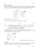
(14.8)
Upon examining Figure 14.2, it can be seen that

n

x



=



dy

/

ds

and

n

y



=




−

dx

/

ds

, in
which

s

is the arc length along the boundary at

z

. Consequently,
(14.9)
Now, on and therefore

ψ

is a constant, which can, in general, be taken
as zero.
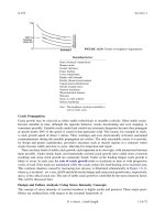
We next consider the total torque on the member. Figure 14.3 depicts the cross
section at

z


. The torque on the element at

x

and

y

is given by
(14.10)

FIGURE 14.2

Illustration of geometric relation.
ψ
ψ
dψ
z
–dx
dy
ds
n
n
x
= cos
χ
= dy/ds
n
y

= sin
χ
= dx/ds
∂
∂
+
∂
∂
=−
2
2
2
2
2
ψψ
µ
θ
xy
d
dz
.
τ
z x xz y yz
nS nS S=+=0 on .
τ
ψψ
ψ
zxzyz
dy
ds

S
dx
ds
S
dy
ds y
dx
ds x
d
ds
=−
=
∂
∂
+
∂
∂
=
S
d
ds
,
ψ
= 0,
dT xS dxdy yS dxdy
x
d
dx
y
d

dy
dxdy
yz xz
=−
=− −






ψψ

0749_Frame_C14 Page 183 Wednesday, February 19, 2003 5:41 PM
© 2003 by CRC CRC Press LLC

184

Finite Element Analysis: Thermomechanics of Solids

Integration furnishes
(14.11)
Application of the divergence theorem to the first term leads to

∫

ψ

[


xn

x



+



yn

y

]

ds

,
which vanishes since

y

vanishes on

S

. Finally,
(14.12)
We apply variational methods to the Poisson Equation, considering the stress-

potential function

y

to be the unknown. Now,
(14.13)

FIGURE 14.3

Evaluation of twisting moment.
z
x
x
y
y
dx
s
yz
s
xz
dy
Tx
d
dx
y
d
dy
dxdy
dx
dx

dy
dy
dx
dx
dy
dy
dxdy
x
y
dxdy dxdy
=− +






=− +






−+













=− ∇⋅






+
∫
∫
∫∫
ψψ
ψψ
ψ
ψ
ψ
ψ
() ()
2
T dxdy=
∫
2
ψ

.
δψ ψ µθ
[].∇⋅∇ +
′
=
∫
20dxdy

0749_Frame_C14 Page 184 Wednesday, February 19, 2003 5:41 PM
© 2003 by CRC CRC Press LLC

Torsion and Buckling

185

Integration by parts, use of the divergence theorem, and imposition of the
“constraint”

y



=

0 on

S

furnishes
(14.14)

The integrals are evaluated over a set of small elements. In the

e

th

element,
approximate

ψ

as in which

ν

T

is a vector with dimension (number of
rows) equal to the number of nodal values of

ψ

. The gradient

∇

ψ

has a corresponding
interpolation model in which ββ

ββ

T

is a matrix. The finite-element
counterpart of the Poisson Equation at the element level is written as
(14.15)
and the stiffness matrix should be nonsingular, since the constraint

y



=

0 on

S

has
already been used. It follows that, globally, The torque satisfies
(14.16)
In the theory of torsion, it is common to introduce the torsional constant

J,

for
which

T




=

2

µ

J

θ

′

. It follows that

14.2 BUCKLING OF BEAMS AND PLATES
14.2.1 E

ULER

B

UCKLING



OF


B

EAM

C

OLUMNS

14.2.1.1 Static Buckling

Under in-plane compressive loads, the resistance of a thin member (beam or plate)
can be reduced progressively, culminating in

buckling

. There are two equilibrium
states that the member potentially can sustain: compression only, or compression
with bending. The member will “snap” to the second state if it involves less “potential
energy” than the first state. The notions explaining buckling are addressed in detail in
subsequent chapters. For now, we will focus on beams and plates, using classical
equations in which, by retaining lowest-order corrections for geometric nonlinearity,
in-plane compressive forces appear.
() .∇⋅∇ =
′
∫∫
δψ ψ δψ µθ
dxdy dxdy2
ν
Tee
xy

T
(,) ,ψψηη
∇=
ψ
ββψψηη
Tee
xy
T
(,) ,
Kf
K
f
TT
T
T
e
eT
e
T
e
eTT e
T
e
eT
dxdy
x y dxdy
() ()
()
()
(,)

ηη
ψψββββψψ
ψψ
=
′
=
=
∫
∫
2
µθ
ν

ηη
g
g
1
g
Kf=
′
−
2
µθ

TT
() ()
.
T dxdy
T
TTT

=
=
=
′
∫
()
()()
−
()
2
2
4
ψ
µθ
ηη
g
T
g
g
T
g
1
g
f
fKf
J
T
g
T
g

T
g
T
=
−
2
1
fKf
() () ()
.

0749_Frame_C14 Page 185 Wednesday, February 19, 2003 5:41 PM
© 2003 by CRC CRC Press LLC

186

Finite Element Analysis: Thermomechanics of Solids

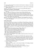
For the beam shown in Figure 14.4, the classical Euler buckling equation is
(14.17)
and

P

is the axial compressive force. The interpolation model for

w(x) is recalled
as w(x) = ϕϕ
ϕϕ
T

(x)ΦΦ
ΦΦ
γγ
γγ
. Following the usual variational procedures (integration by parts)
furnishes
(14.18)
At x = 0, both
δ
w and −
δ
w′ vanish, while the shear force V and the bending
moment M are identified as V = −EIw′′′ and M = −EIw′′. The “effective shear force”
Q is defined as Q = −Pw′ − EIw′′′.
For the specific case illustrated in Figure 14.3, for a one-element model, we can
use the interpolation formula
(14.19)
The mass matrix is shown, after some algebra, to be
(14.20)
FIGURE 14.4 Euler buckling of a beam column.
z
E,
I,A,L,
ρ
y
x
Q
0
M
0

P
EIw Pw Aw
iv
+
′′
+=
ρ
˙˙
,0
δρ δ ρ
wAwdx x A xdV
˙˙
˙˙
,()()
∫∫
→=γγγγΦΦϕϕϕϕΦΦ
TTT
MM
δδδ
δδ
w Iw Pw dx w Iw dx wPwdx
wPw Iw w Iw
iv
LL
[]
[( )( )] [( )( )]
EE
EE
+
′′

=
′′ ′′
−
′′
−−
′
−
′′′
−−
′
−
′′
∫∫∫
00
wx x x
LL
LL
tt
wL
wL
( ) ( ) () ()
()
()
.=
−−









=
−
′






−
23
23
2
1
23
γγγγ,
MKK==








ρ
AL

L
LL
00
2
13
35
11
210
11
210
1
105
,.
0749_Frame_C14 Page 186 Wednesday, February 19, 2003 5:41 PM
© 2003 by CRC CRC Press LLC
Torsion and Buckling 187
Similarly,
(14.21)
The governing equation is written in finite-element form as
(14.22)
In a static problem, the solution has the form
(14.23)
in which cof denotes the cofactor, and γγ
γγ
→ ∞ for values of which render
det(K
2

14.2.1.2 Dynamic Buckling
In a dynamic problem, it may be of interest to determine the effect of P on the

resonance frequency. Suppose that f(t) = f
0
exp(i
ω
t), in which f
0
is a known vector.
The displacement function satisfies γγ
γγ
(t) = γγ
γγ
0
exp(i
ω
t), in which the amplitude vector
γγ
γγ
0
satisfies
(14.24)
Resonance occurs at a frequency
ω
0
, for which
(14.25)
Clearly, is an eigenvalue of the matrix The
resonance frequency is reduced by the presence of P and vanishes precisely at
the critical value of P.
δδ
δδ

′′
==








′′ ′′
==








∫
∫
wPwdx
P
L
L
LL
wIwdx
I
L

L
LL
T
T
γγγγ
γγγγ
KK
KK
11
2
3
22
2
6
5
1
10
1
10
2
15
12 6
64
,
E
E
,
E
,
I

L
P
L
AL
Q
M
3
21 0
0
0
KK Kf f−






+==






γγγγ
ρ
˙˙
.
˙˙
,γγ=0

γγ=
−






−






cof
det
,
KK
KK
f
21
21
PL
I
PL
I
2
2
E

E
PL
I
2
E
−=
PL
I
2
1
0
E
K ).
EI
L
P
L
AL
3
21
2
00 0
KK K f−−






=

ωρ
γγ .
det .
EI
L
P
L
AL
3
210
2
0
0KK K−−






=
ωρ
ω
0
2
1
0
12
210
12
3

ρ
AL
E
KKKK
−−
−
//
[].
I
L
P
L
ω
0
2
0749_Frame_C14 Page 187 Wednesday, February 19, 2003 5:41 PM
© 2003 by CRC CRC Press LLC
188 Finite Element Analysis: Thermomechanics of Solids
14.2.1.3 Sample Problem: Interpretation of Buckling Modes
Consider static buckling of a clamped-clamped beam, as shown in Figure 14.5.
This configuration can be replaced with two beams of length L, for which the
right beam experiences shear force V
1
and bending moment M
1
, while the left beam
experiences shear force V
0
− V
1

and bending moment M
0
− M
1
. The beam on the
right is governed by
(14.26)
The governing equation is written in finite-element form as
(14.27)
Consider the symmetric case in which M
0
= 0, with the implication that w′(L) = 0.
The equation reduces to
(14.28)
from which we obtain the critical buckling load given by P
1
= 10EI/L
2
.
FIGURE 14.5 Buckling of a clamped-clamped beam.
LL
M
0
V
0
P
δδ
δδ
′′
==









′′ ′′
==








∫
∫
wPwdx
P
L
L
LL
wIwdx
I
L
L
LL

T
T
γγγγ
γγγγ
KK
KK
11
2
3
22
2
6
5
1
10
1
10
2
15
12 6
64
,
E
E
,
EI
L
L
LL
P

L
L
LL
3
2
2
12 6
64
6
5
1
10
1
10
2
15








−

















=γγ f
f =






=
−
′






V
M

wL
wL
1
1
,
()
()
γγ
12
6
5
3
1
EI
L
P
L
wL V−






=() ,
0749_Frame_C14 Page 188 Wednesday, February 19, 2003 5:41 PM
© 2003 by CRC CRC Press LLC
Torsion and Buckling 189
Next, consider the antisymmetric case in which V
0

= 0 and w(L) = 0. The coun-
terpart of Equation 14.28 is now
(14.29)
and P
2
= 30EI/L
2
.
If neither the constraint of symmetry nor axisymmetry is applicable, there are two
critical buckling loads, to be obtained in Exercise 2 as and These values
are close enough to the symmetric and antisymmetric cases to suggest an interpretation
of the two buckling loads as corresponding to the two “pure” buckling modes.
Compare the obtained values with the exact solution, assuming static condi-
tions. Consider the symmetric case. Let w(x) = w
c
(x) + w
p
(x), in which w
c
(x) is
the characteristic solution and w
p
(x) is the particular solution reflecting the per-
turbation. From the Euler buckling equation demonstrated in Equation 14.17, w
c
(x)
has a general solution of the form w
c
(x) =
α

+
β
x +
γ
cos
κ
x +
δ
sin
κ
x, in which
κ
= Now, w = −w′ = 0 at x = 0, −w′(L) = 0, and EIw′′′(L) = V
1
, expressed
as the conditions
(14.30)
or otherwise stated
(14.31)
For the solution to “blow up,” it is necessary for the matrix B to be singular,
which it is if the corresponding homogeneous problem has a solution. Accordingly,
we seek conditions under which there exists a nonvanishing vector z, for which Bz = 0.
Direct elimination of
α
and
β
furnishes
α
= −
γ

and
β
= −
κδ
. The remaining
coefficients must satisfy
(14.32)
4
2
15
1
EI
L
PL w L M−






−
′
=( ( )) ,
27 8
2
.
EI
L
89
2


EI
L
PL I
2
/.E
1010 0
010 0
0
00
33
1
αβγδ
αβγκδ
αβγκκδκκ
αβγκ κδκ κ
+++=−
+++=−
′
+− + =−
′
++ − =−
′′′
+
w
w
LLLwL
L L EIw L V
p
p

p
p
()
()
sin cos ( )
sin cos ( )

Bz B z=
−
−
′
−
′
−
′′′
+

















=
−
−
















=




w
w
wL
Iw L V

LLL
LL
p
p
p
p
()
()
()
()
sin cos
sin cos
,
0
0
10 1 0
01 0
0
00
1
33
E
,
κ
κκ κ κ
κκ κκ
α
β
γ
δ











−−














=







sin cos
sin cos
.
κκκ
κκ
γ
δ
LLL
LL
0
0
0749_Frame_C14 Page 189 Wednesday, February 19, 2003 5:41 PM
© 2003 by CRC CRC Press LLC
190 Finite Element Analysis: Thermomechanics of Solids
A nonvanishing solution is possible only if the determinant vanishes, which
reduces to sin
κ
L = 0. This equation has many solutions for kL, including kL = 0.
The lowest nontrivial solution is kL = p, from which P
crit
=
π
2
EI/L
2
= 9.87 EI/L
2
.

Clearly, the symmetric solution in the previous two-element model (P
crit
= 10 EI/L
2
)
gives an accurate result.
For the antisymmetric case, the corresponding result is that tan
κ
L =
κ
L. The
lowest meaningful root of this equation is kL = 4.49 (see Brush and Almroth, 1975),
giving P
crit
= 20.19 EI/L
2
. Clearly, the axisymmetric part of the two-element model is
not as accurate, unlike the symmetric part. This issue is addressed further in the
subsequent exercises.
Up to this point, it has been implicitly assumed that the beam column is initially
perfectly straight. This assumption can lead to overestimates of the critical buckling
load. Consider a known initial distribution w
0
(x). The governing equation is
(14.33)
or equivalently,
(14.34)
The crookedness is modeled as a perturbation. Similarly, if the cross-sectional
properties of the beam column exhibit a small amount of variation, for example,
EI(x) = EI

0
[1 +
ϑ
sin(
π
x/L)], the imperfection can also be modeled as a perturbation.
14.2.2 EULER BUCKLING OF PLATES
The governing equation for a plate element subject to in-plane loads is
(14.35)
(see Wang 1953), in which the loads are illustrated as shown in Figure 14.6. The usual
FIGURE 14.6 Plate element with in-plane compressive loads.
d
dx
I
d
dx
ww P
d
dx
ww
2
2
2
2
0
2
2
0
0E( ) ( ),−+ −=
d

dx
I
d
dx
wP
d
dx
w
d
dx
I
d
dx
wP
d
dx
w
2
2
2
2
2
2
2
2
2
2
0
2
2

0
EE+= +.
Eh
wP
w
x
P
w
y
P
w
xy
xyxy
2
2
4
2
2
2
2
2
12 1
0
()−
∇+
∂
∂
+
∂
∂

+
∂
∂∂
=
ν
z
x
P
x
P
yx
P
y
P
xy
h
y
0749_Frame_C14 Page 190 Wednesday, February 19, 2003 5:41 PM
© 2003 by CRC CRC Press LLC
Torsion and Buckling 191
variational methods furnish, with some effort,
(14.36)
in which W = ∇∇
T
w (a matrix!). In addition,
(14.37)

For simplicity’s sake, assume that from which we can obtain
the form
(14.38)

We also assume that the secondary variables (n ⋅ ∇)∇
2
w, (n ⋅ ∇)∇w, and also
are prescribed on S.
These conditions serve to obtain
(14.39)
and f reflects the quantities prescribed on S.
As illustrated in Figure 14.7, we now consider a three-dimensional loading space
in which P
x
, P
y
, and P
xy
correspond to the axes, and seek to determine a surface in
the space of critical values at which buckling occurs. In this space, a straight line
δδ δ δ
w w dA w w dS w w dS tr dA∇ = ⋅∇ ∇ − ∇ ⋅ ⋅∇ ∇ +
∫∫ ∫ ∫
42
() ( ) ( ),nnPWW
δ
δδ
wP
w
x
P
w
y
P

w
xy
dA dw n n dS
ww
w
w
dA
xy
xy
x
y
xyxy

∂
∂
∂
∂
∂
∂∂
2
2
2
2
2
++







=
−






∫∫
∫
()
{},
p
P
pP=
+
[]
+
[]








=









∂
∂
∂
∂
∂
∂
∂
∂
PP
PP
PP
PP
xxy
xy y
xxy
xy y
w
x
w
y
w
x
w

y
1
2
1
2
1
2
1
2
,
wxy
bbb
(,)=ϕϕΦΦγγ
222
T
∇=






=
()
=w
w
w
VEC
x
y

bbb bbb
ββΦΦγγββΦΦγγ
12 22 2222
TT
W,
.
[]
[]
PP
PP
xxy
xy y
w
x
w
y
w
x
w
y
∂
∂
∂
∂
∂
∂
∂
∂
+
+









1
2
1
2
[]KK f
bbb21 22 2
−=γγ
K
K
TT
TT
bbbbb
bbbbb
E
d
d
21
2
2
22222 2
22 2 1 2 1 2 2
12 1

=
−
=
∫
∫
h
A
()
ν
ΦΦββββΦΦ
ΦΦββββΦΦP V
0749_Frame_C14 Page 191 Wednesday, February 19, 2003 5:41 PM
© 2003 by CRC CRC Press LLC
192 Finite Element Analysis: Thermomechanics of Solids
emanating from the origin represents a proportional loading path. Let the load
intensity,
λ
, denote the distance to a given point on this line. By analogy with
spherical coordinates, there exist two angles,
θ
and
φ
, such that
(14.40)
Now,
(14.41)
For each pair (q, f), buckling occurs at a critical load intensity,
λ
crit
(

θ
,
φ
),
satisfying
(14.42)
A surface of critical load intensities,
λ
crit
(
θ
,
φ
), can be drawn in the loading space
shown in Figure 14.7 by evaluating
λ
crit
(
θ
,
φ
) over all values of (q, f) and discarding
values that are negative.
FIGURE 14.7 Loading space for plate buckling.
P
xy
P
y
P
x

λ
φ
θ
PPP
xyxy
===
λθφ λθφ λφ
cos cos , sin cos , sin
KK
KP
P
TT
bb
bbbbb
dV
22 22
22 2 1 2 1 2 2
=
=
=








∫
λθϕ

θϕ θϕ
θφ
θϕ ϕ
ϕθϕ
ˆ
(, )
ˆ
(, )
ˆ
(, )
ˆ
(, )
cos sin
sin sin
ΦΦββββΦΦ
cos
cos
det[ ( , )
ˆ
].KK
b
crit
b21 22
0−=
λθφ
0749_Frame_C14 Page 192 Wednesday, February 19, 2003 5:41 PM
© 2003 by CRC CRC Press LLC
Torsion and Buckling 193
14.3 EXERCISES
1. Consider the triangular member shown to be modeled as one finite ele-

ment. Assume that
Find K
T
, f
T
, and the torsional constant T.
2. Find the torsional constant for a unit square cross section using two
triangular elements.
3. Derive the matrices K
0
, K
1
, and K
2
in Equations 14.20 and 14.21.
4. Compute the two critical values in Equation 14.23.
5. Use the four-element model shown in Figure 14.5, and determine how much
improvement, if any, occurs in the symmetric and antisymmetric cases.
6. Consider a two-element model and a four-element model of the simple-
simple case shown in the following figure. Compare P
crit
in the symmetric
and antisymmetric cases with exact values.
Triangular shaft cross section.
ψ
ψ
ψ
ψ
(,) ( ) .xy x y
xy

xy
xy
=
























−
1
1

1
1
11
22
33
1
1
2
3
y
x
(2,3)
(3,2)
(1,1)
V
0
M
0
LL
P
0749_Frame_C14 Page 193 Wednesday, February 19, 2003 5:41 PM
© 2003 by CRC CRC Press LLC
194 Finite Element Analysis: Thermomechanics of Solids
7. Consider a cantilevered beam with a compressive load P, as shown in the
following figure. The equation is
The primary variables at x = L are w(L) and −w′(L), and
Find the critical buckling load(s).
EI
dw
dx

P
dw
dx
4
4
2
2
0+=.
δδ δδ
′′ ′′
=








′′
=








∫∫

wIwdx
I
L
L
LL
wPwdx
P
L
L
LL
L
E
E
0
L
0
3
22
12 6
64
12 6
64
γγγγγγγγ
TT
,.
L
V
0
M
0

P
0749_Frame_C14 Page 194 Wednesday, February 19, 2003 5:41 PM
© 2003 by CRC CRC Press LLC