139

Element and Global
Stiffness and Mass
Matrices

10.1 APPLICATION OF THE PRINCIPLE
OF VIRTUAL WORK

Elements of variational calculus were discussed in Chapter 3, and the Principle of
Virtual Work was introduced in Chapter 5. Under static conditions, the principle is
repeated here as
(10.1)
As before,

δ

represents the variational operator. We assume for our purposes
that the displacement, the strain, and the stress satisfy representations of the form
(10.2)
in which

E

and

S

are written as one-dimensional arrays in accordance with traditional
finite-element notation. For use in the Principle of Virtual Work, we need

D

′

, which
introduces the factor 2 into the entries corresponding to shear. We suppose that the
boundary is decomposed into four segments: S

=

S

I



+

S

II



+

S

III




+

S

IV

. On S

I

,

u

is
prescribed, in which event

δ

u

vanishes. On S

II

, the traction ττ
ττ


is prescribed as ττ
ττ

0

.
On S

III

, there is an elastic foundation described by ττ
ττ



=

ττ
ττ

0



−



A


(

x

)

u

, in which

A

(

x

) is
a known matrix function of

x

. On S

IV

, there are inertial boundary conditions, by
virtue of which ττ
ττ




=

ττ
ττ

0



−



Bü

. The term on the right now becomes
(10.3)
1
0
δδρδτ
ESdV u udV u dS
ij ij i i i i
∫∫∫
+=
˙˙
.
ux ) x
T

(()() ()(),t t , t , ,===ϕϕΦΦγγββΦΦγγESE
T
xD
δτ δ
δ
δ
udS dS
dS t
dS t
ii
∫∫
∫
∫
=
−
−
++
γγΦΦϕϕττ
γγΦΦϕϕϕϕΦΦγγ
γγΦΦϕϕϕϕΦΦγγ
TT
0
TT T
TT T
x
xA x
xB x
()
() () ()
() ()

˙˙
().
SS S
S
S
II III IV
III
IV



0749_Frame_C10 Page 139 Wednesday, February 19, 2003 6:04 PM
© 2003 by CRC CRC Press LLC

140

Finite Element Analysis: Thermomechanics of Solids

The term on the left in Equation 10.1 becomes
(10.4)
in which

K

is called the stiffness matrix and

M

is called the mass matrix. Canceling
the arbitrary variation and bringing terms with unknowns to the left side furnishes

the equation as follows:
(10.5)
Clearly, elastic supports on S

III

furnish a boundary contribution to the stiffness
matrix, while mass on the boundary segment S

IV

furnishes a contribution to the mass
matrix.

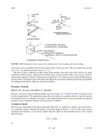
Sample Problem 1: One element rod

Consider a rod with modulus E, mass density

ρ

, area

A

, and length

L

. It is built in
at


x



=

0. At

x



=



L

, there is a concentrated mass

m

to which is attached a spring of
stiffness

k

, as illustrated in Figure 10.1. The stiffness and mass matrices, from the
domain, reduce to the scalar values


K



→



EA

/

L

,

M



→



ρ

AL

/


3,

M

S



→



m

,

K

S



→



k

.

The governing equation is .

Sample Problem 2: Beam element

Consider a one-element model of a cantilevered beam to which a solid disk is welded
at

x



=



L

. Attached at

L

is a linear spring and a torsional spring, the latter having
the property that the moment developed is proportional to the slope of the beam.

FIGURE 10.1

Rod with inertial and compliant boundary conditions.
δ
δρ
ESdV

udV
ij ij
ii
∫∫
∫∫
==
′
==
δδγγγγΦΦββββΦΦ
δδγγγγρρΦΦϕϕϕϕΦΦ
TTT
TTT
KKxDx
MM xx
(), ( ) ( )
˙˙
˙˙
(), ( ) ( ) ,
t dV
ut dV
()()( )
˙˙
KK MM f+++ =
SS
ttγγγγ()
fx
KxAx
MxBx
T
0

TT
TT
=
=
=
+
∫
∫
∫
ΦΦϕϕττ
ΦΦϕϕϕϕΦΦ
ΦΦϕϕϕϕΦΦ
()
() ()
() () .
dS
dS
dS
S
S
SS
S
S
II III
III
IV
()( )
˙˙
EA
L

AL
kmf++ + =
γγ
ρ
3
E,A,L,ρ
P
m
k

0749_Frame_C10 Page 140 Wednesday, February 19, 2003 6:04 PM
© 2003 by CRC CRC Press LLC

Element and Global Stiffness and Mass Matrices

141

The shear force

V

0

and the moment

M

0

act at


L

. The interpolation model, incorpo-
rating the constraints

w

(0,

t

)

=



−

w

′

(0,

t

)


=

0

a priori

, is
(10.6)
The stiffness and mass matrices, due to the domain, are readily shown to be
(10.7)
The stiffness and mass contributions from the boundary conditions are
(10.8)
The governing equation is now
(10.9)

10.2 THERMAL COUNTERPART OF THE PRINCIPLE
OF VIRTUAL WORK

For our purposes, we focus on the equation of conductive heat transfer as
. (10.10)

FIGURE 10.2

Beam with translational and rotational inertial and compliant boundary conditions.
z
y
E,I,A,L,ρ
M
0
k

T
k
x
V
0
m
r
wxt xx
LL
LL
wLt
wLt
(,) ( )
(,)
(,)
.=
−−








−
′







−
23
23
2
1
23
KM=








=








EI
L
L

LL
AL
L
LL
3
2
13
35
11
210
11
210
1
105
2
12 6
64
,.
ρ
KM
S
T
S
mr
k
k
m
=









=








0
0
0
0
2
2
,
.

()
˙˙
(,)
˙˙
(,)
()

(,)
(,)
.MM KK+
−
′






++
−
′






=






SS
wLt
wLt

wLt
wLt
V
M
0
0
kc
t
e
∇=
∂
∂
2
T
T
ρ

0749_Frame_C10 Page 141 Wednesday, February 19, 2003 6:04 PM
© 2003 by CRC CRC Press LLC

142

Finite Element Analysis: Thermomechanics of Solids

Multiplying by the variation of

T




−



T

0

, integrating by parts, and applying the
divergence theorem furnishes
(10.11)
Now suppose that the interpolation models for temperature in the current element
furnish a relation of the form
. (10.12)
The terms on the left in Equation 10.11 can now be written as
(10.13)

K

T

and

M

T

can be called the thermal stiffness (or conductance) matrix and thermal
mass (or capacitance) matrix, respectively.
Suppose that the boundary


S

has four zones: S

=

S

I



+

S

II



+

S

III



+


S

IV

. On S

I

, the
temperature is prescribed as T

1

, from which we conclude that

δ

T

=

0. On S

II

, the
heat flux is prescribed as

n


T

q

1

. On S

III

,

the heat flux satisfies

n

T

q



=



n

T


q

1



−

h
1
(T −
T
0
), while on S
IV
, n
T
q = n
T
q
1
− h
2
d T/dt. The governing finite-element equation is
now
(10.14)
10.3 ASSEMBLAGE AND IMPOSITION
OF CONSTRAINTS
10.3.1 R

ODS
Consider the assemblage consisting of two rod elements, denoted as e and e + 1
[see Figure 10.3(a)]. There are three nodes, numbered n, n + 1, and n + 2. We first
consider assemblage of the stiffness matrices, based on two principles: (a) the forces
at the nodes are in equilibrium, and (b) the displacements at the nodes are continuous.
Principle (a) implies that, in the absence of forces applied externally to the node, at
node n + 1, the force of element e + 1 on element e is equal to and opposite the force
of element e on element e + 1. It is helpful to carefully define global (assemblage
δδρδ
∇∇ +
∂
∂
=
∫∫ ∫
TT
nqTT T
T
TkdV c
t
dV dS
e
.
TT T −= ∇= =−
0
ϕϕΦΦθθββΦΦθθΦΦθθ
TT TT T T
ttkt
TTT
xxqx() (), () (), () ()
δδ

δρ δ ρ
∇∇ → =
∂
∂
→=
∫∫
∫∫
T
TTTTTT
eTTeTTTT
kdV t t k dV
c
t
dV t t c dV
TT
T
T

θθθθΦΦββββΦΦ
θθθθΦΦϕϕϕϕΦΦ
TTT
TTT
KK
MM
() (),
()
˙
(), .
[]
˙

() [ ]() ()MM KK f
TTS TTS T
ttt+++=θθθθ
MK
fnq
TT
TS T
T
TT
T
TTSTTTT
TT
T
T
T
hdS hdS
tdS
==
==++
∫∫
∫
ΦΦϕϕϕϕΦΦΦΦϕϕϕϕΦΦ
ΦΦϕϕ
21
1
SS
II III IV
IV III

S S S

,
() ,
Ω
Ω
0749_Frame_C10 Page 142 Wednesday, February 19, 2003 6:04 PM
© 2003 by CRC CRC Press LLC
Element and Global Stiffness and Mass Matrices 143
level) and local (element level) systems of notation. The global system of forces is
shown in (a), while the local system is shown in (b). At the center node,
(10.15)
since no external load is applied. Clearly, .
The elements satisfy
(10.16)
and in this case, k
(e)
= k
(e+1)
= EA/L. These relations can be written as four separate
equations:
(10.17)
FIGURE 10.3 Assembly of rod elements.
P
n
P
n+2
P
1
(e+1)
P
2

(e+1)
P
1
(e)
P
2
(e)
n n+1
e+1e
e e+1
a. forces in global system
b. forces in local system
PP
ee
12
1
0
() ( )
−=
+
PP P P
e
n
e
n21
1
2
() ( )
==
+

+
and
k
u
u
P
P
k
u
u
P
P
e
n
n
e
e
e
n
n
e
e
()
()
()
()
()
()
11
11

11
11
1
2
1
1
1
2
2
1
1
1
−
−














=
−









−
−














=
−









+
+
+
+
+
+
ku ku P
ku ku P
ku ku P
ku ku P
e
n
e
n
e
e
n
e
n
e
e
n
e
n
e
e

n
e
n
e
() () ()
() () ()
() () ()
() () ()
(
(
(
−=−
−+ =
−=−
−+ =
+
+
+
+
+
+
+
+
+
+
+
+
12
11
1

1
1
22
1
1
1
1
21
1
i)
ii)
iii)
iv)(
0749_Frame_C10 Page 143 Wednesday, February 19, 2003 6:04 PM
© 2003 by CRC CRC Press LLC
144 Finite Element Analysis: Thermomechanics of Solids
Add (ii) and (iii) and apply Equation 10.15 to obtain
(10.18)
and in matrix form
(10.19)
The assembled stiffness matrix shown in Equation 10.19 can be visualized as
an overlay of two element stiffness matrices, referred to global indices, in which
there is an intersection of the overlay. The intersection contains the sum of the lowest
entry on the right side of the upper matrix and the highest entry on the left side of
the lowest matrix. The overlay structure is depicted in Figure 10.4.
FIGURE 10.4 Assembled beam stiffness matrix.
ku ku P
ku k k u k u
ku ku P
e

n
e
n
e
e
n
ee
n
e
n
e
n
e
n
e
() () ()
() () ( ) ( )
() () ()
[]
(
(
(
−=−
−++ − =
−−=
+
+
+
+
+

+
+
+
+
+
+
12
1
1
1
2
1
1
1
21
1
0


i)
ii iii)
iv)
kk
kkk k
kk
u
u
u
P
P

ee
eee e
ee
n
n
n
n
n
() ()
() () ( ) ( )
() ()

−
−+−
−

























=
−












++
++
+
++
0
0
0

11
11
1
21
K
(1)
K
(2)
K
(3)
K
(4)
k
22
+k
11
K
(5)
K
(N–2)
K
(N–1)
K
(N)
(4) (5)
0749_Frame_C10 Page 144 Wednesday, February 19, 2003 6:04 PM
© 2003 by CRC CRC Press LLC
Element and Global Stiffness and Mass Matrices 145
Now, the equations of the individual elements are written in the global system as
(10.20)

The global stiffness matrix (the assembled stiffness matrix K
(g)
of the two-element
member) is the direct sum of the element stiffness matrices: .
Generally, K
(g)
= ∑
e
. In this notation, the strain energy in the two elements
can be written in the form
(10.21)
The total strain energy of the two elements is
Finally, notice that K
(g)
is singular: the sum of the rows is the zero vector, as is
the sum of the columns. In this form, an attempt to solve the system will give rise
to “rigid-body motion.” To illustrate this reasoning, suppose, for simplicity’s sake,
that k
(e)
= k
(e+1)
, in which case equilibrium requires that P
n
= P
n+2
. If computations
were performed with perfect accuracy, the equation would pose no difficulty. How-
ever, in performing computations, errors arise. For example, P
n
is computed as

and . Computationally, there is now an
unbalanced force, . In the absence of mass, this, in principle, implies infinite
accelerations. In the finite-element method, the problem of rigid-body motion can
be detected if the output exhibits large deformation.
The problem is easily suppressed using constraints. In particular, symmetry
implies that u
n+1
= 0. Recalling Equation 10.19, we now have
, (10.22)
in which R is a reaction force that arises to enforce physical symmetry in the presence
of numerically generated asymmetry. The equation corresponding to the second
equation is useless in predicting the unknowns u
n
and u
n+2
since it introduces the
KKK K
KK
eee e
ee
() () ( ) ( )
() () ( ) ( )
˜
,
˜
˜
,
˜
.
→→

=
−
−












=−
−












++

++


11
11
110
110
000
00 0
01 1
011
kk
ee
KKK
gee() () ( )
˜˜
=+
+1
˜
()
K
e
VK
VK
eeee
eeee
e
T
() () () ()
() () ()()

()
˜
˜
().
=
=
=
++
++
1
2
1
2
11
12
γγγγ
γγγγ
γγ
ΤΤ
ΤΤ
uu u
nn n
1
2
γγγγ
Tg
K
()
.
ˆ

PP
nnn
=+
ε
ˆ
,PP PPP
nnnnn++++
=+ ==
1111
ε

εε
n
n
+
−
1
EA
L
u
u
P
R
P
n
n
n
n
110
12 1

011
0
21
−
−−
−

























=
−












++

0749_Frame_C10 Page 145 Wednesday, February 19, 2003 6:04 PM
© 2003 by CRC CRC Press LLC
146 Finite Element Analysis: Thermomechanics of Solids
new unknown R. The first and third equations are now rewritten as
, (10.23)
with the solution
. (10.24)
To preserve symmetry, it is necessary for u
n
+ u
n+1
= 0. However, the sum is
computed as
(10.25)

The reaction force is given by R = −[
ε
n
+
ε
n+1
], and, in this case, it can be considered
as a measure of computational error.
Note that Equation 10.23 can be obtained from Equation 10.22 by simply “striking
out” the second row of the matrices and vectors and the second column of the matrix.
The same assembly arguments apply to the inertial forces as to the elastic forces.
Omitting the details, the kinetic energies T of the two elements are
(10.26)
10.3.2 BEAMS
A similar argument applies for beams. The potential energy and stiffness matrix of
the e
th
element can be written as
(10.27)
EA
L
u
u
P
P
n
n
n
n
10

01
11














=
−+
+






++
ε
ε
uP
A

L
uP
A
L
nn n n
=− + = +
++
[] []
εε
E
,
E
21
uu
nn
nn
A
L
+=
+
()
+
+
1
1
εε
E
.
T =+
+

1
2
1
˙
[
˜˜
˙
() () ( ) ()
γγ]]γγ
ee ee
T
MM
˜
/
/
˙
{
˙˙ ˙
}
() ()
()
()
()
M
ee
e
e
e
T
=









=






=
++
m
mAl
uu u
ee e
112
12 1
1
3
12
ρ
γγ
V
www w

bb
b
eee e
() ()
()
() ()
() ()
{}
ee
e
11
e
12
e
21
eT
22
e
T
K
K
KK
KK
=
=











=−
′
−
′
++
1
2
11
γγγγ
γγ
T
0749_Frame_C10 Page 146 Wednesday, February 19, 2003 6:04 PM
© 2003 by CRC CRC Press LLC
Element and Global Stiffness and Mass Matrices 147
In a two-element beam model analogous to the previous rod model, V
(g)
= V
(e)
+
V
(e+1)
, implying that
. (10.28)
Generally, in a global coordinate system, K
(g)

= ∑∑
∑∑
e
K
(e)
.
10.3.3 TWO-DIMENSIONAL ELEMENTS
We next consider assembly in 2-D. Consider the model depicted in Figure 10.5
consisting of four rectangular elements, denoted as element e, e + 1, e + 2, and e + 3.
The nodes are also numbered in the global system. Locally, the nodes in an element
are numbered in a counterclockwise fashion. Suppose there is one degree of freedom
per node (e.g., x-displacement) and one corresponding force.
FIGURE 10.5 2-D assembly process.
K
KK 0
KKK K
0K K
g
11
e
12
e
21
eT
22
e
11
e
12
e

21
eT
22
e
()
() ()
() () ( ) ( )
() ()
=+










++
++
11
11
e+3,4
e+3,1 e+3,2 e+2,1 e+2,2
e+1,3
e+1,2e+1,1e,2e,1
e,4 e,3
e+2,4
e+1,4

e+2,3
e+3
e+3
e+2
e+2
e
e
e+1
e+1
e+3,3
789
123
6
5
4
0749_Frame_C10 Page 147 Wednesday, February 19, 2003 6:04 PM
© 2003 by CRC CRC Press LLC
148 Finite Element Analysis: Thermomechanics of Solids
In the local systems, the force on the center node induces displacements according to
(10.29)
Globally,
(10.30)
Adding the forces of the elements on the center node gives
(10.31)
Taking advantage of the symmetry of the stiffness matrix, this implies that the
fifth row of the stiffness matrix is
(10.32)
Finally, for later use, we consider damping, which generates a stress proportional
to the strain rate. In linear problems, it leads to a vector-matrix equation of the form
. (10.33)

At the element level, the counterpart of the kinetic energy and the strain energy
is the Rayleigh Damping Function, D
(e)
, given by , and the con-
sistent damping force on the e
th
element is
(10.34)
fkukukuku
fkukukuku
e
e
e
e
e
e
e
e
e
e
e
e
e
e
e
e
e
,
() () () ()
() () () ()

3311322333 344
14 41
1
11 4 2
1
12 43
1
13 44
1
=+++
=+++
+
+
+
+
+
+
+
+
,, ,, ,, ,,
,, ,, ,, ,,ee
e,
e
e
e
e
e
e
e
e

e
e
e
e
e
fkukukuku
fkukuk
+
+
+
+
+
+
+
+
+
+
+
+
+
+
+
=+++
=++
14
21 11
2
21 12
2
22 13

2
23 14
2
24
32 21
3
31 2 2
3
32 2
,
,,,,,,,,
,, ,, ,
() () () ()
() ()
,, , , ,3
3
33 24
3
34
() ()e
e
e
e
uku
+
+
+
+
+
uu uu uu uu

uuuuuuuu
uuuuuuu u
uuu
eeee
eeee
eeee
ee
,,,,
,,,,
,,,,
,,
11 2 2 3
5
4
6
11 2 12 3 13 4 14
5
21
5
22 4 23 9 24 8
31
6
32
→→→→
→→→→
→→→→
→→
++++
++++
++

uuu uu u
ee
5
33 8 34 7++
→→
,,
fkukkukuk ku
kk k kuk
eee e ee
ee e e
5
31 1 32 41
1
242
1
343
1
12
2
4
33 44
1
11
2
22
3
5
3
=++
[]

+++
[]
++ + +
[]
+
++++
++ +
,
()
,
()
,
()
,
()
,
()
,
()
,
()
,
()
,
()
,
()
,,
()
,

()
,
()
,
()
,
()
,
()
421
3
6
24
3
714
2
23
3
813
2
9
ee
eeee
ku
kuk k uku
+
[]
+++
[]
+

+
++++

κ
5
31 32 41
1
42
1
43
1
12
2
33 44
1
11
2
22
3
T
=+
[]
+
[]
{
+++
[]
}
++++
++ +

kkkkkk
kk kk symmetry
eeeeee
ee e e
,
()
,
()
,
()
,
()
,
()
,
()
,
()
,
()
,
()
,
()
KK
MDKf
˙˙ ˙
()γγγγγγ++=t
D
() () () ()

˙˙
ee
T
ee
D=
1
2
γγγγ
f
d
t
() () () ()
()
˙
˙
.
eeee
D=
∂
∂
=
γγ
γγD
0749_Frame_C10 Page 148 Wednesday, February 19, 2003 6:04 PM
© 2003 by CRC CRC Press LLC
Element and Global Stiffness and Mass Matrices 149
The Rayleigh Damping Function is additive over the elements. Accordingly, if
is the damping matrix of the e
th
element referred to the global system, the

assembled damping matrix is given by
(10.35)
It should be evident that the global stiffness, mass, and damping matrices have
the same bandwidth; the force on one given node depends on the displacements
(velocities and accelerations) of the nodes of the elements connected at the given
node, thus determining the bandwidth.
10.3 EXERCISES
1. The equation of static equilibrium in the presence of body forces, such
as gravity, is expressed by
Without the body forces, the dynamic Principle of Virtual Work is derived as
How should the second equation be modified to include body forces?
2. Consider a one-dimensional system described by a sixth-order differential
equation:
Consider an element from x
e
to x
e+1
. Using the natural coordinate
ξ
= −1
when x = x
e′
= +1 when x = x
e+1
, for an interpolation model with the
minimum order that is meaningful, obtain expressions for ϕϕ
ϕϕ
(
ξ
), ΦΦ

ΦΦ
, and γγ
γγ
,
serving to express q as
.
3. Write down the assembled mass and stiffness matrices of the following
three-element configuration (using rod elements). The elastic modulus is
E, the mass density is
ρ
, and the cross-sectional area is A.
ˆ
()
D
e
DD
ge
e
() ()
ˆ
.=
∑
∂
∂
=−
S
X
b
ij
j

i
.
δδρ δτ
ESdV u
u
t
dV dS
ij ij i
2
i
2
ii
u
∫∫ ∫
+
∂
∂
= .
Q
dq
dx
Q
6
6
0= , a constant.
q
T
() ()
ξξ
=ϕϕΦΦγγ

0749_Frame_C10 Page 149 Wednesday, February 19, 2003 6:04 PM
© 2003 by CRC CRC Press LLC
150 Finite Element Analysis: Thermomechanics of Solids
4. Assemble the stiffness coefficients associated with node n, shown in the
following figure, assuming plane-stress elements. The modulus is E, and
the Poisson’s ratio is . K
(1)
, K
(2)
, and K
(3)
denote the stiffness matrices
of the elements.
5. Suppose that a rod satisfies
δ
Ψ = 0, in which Ψ is given by
Use the interpolation model
For an element x
e
< x < x
e+1
, find the matrix K
e
such that
6. Redo this derivation for K
e
in the previous exercise, using the natural
coordinate
ξ
, whereby

ξ
= ax + b, in which a and b are such that −1 =
ax
e
+ b, +1 = ax
e+1
+ b.
7. Next, regard the nodal-displacement vector as a function of t. Find the
matrix M
e
such that
y
LLL/2
x
ν
K
(1)
K
(3)
K
(2)
n
Ψ=




−
∫
1

2
2
0
du
dx
dx
Pu L
L
()
.
E
ux x
ux t
ux t
e
e
() { }
(,)
(,)
.=






+
1
1
ΦΦ

K
e
e
e
e
e
ux t
ux t
f
f
(,)
(,)
.
++






=






11
MK
e

e
e
e
e
e
e
e
ux t
ux t
ux t
ux t
f
f
(,)
(,)
(,)
(,)
,
+
••
++






+







=






111
0749_Frame_C10 Page 150 Wednesday, February 19, 2003 6:04 PM
© 2003 by CRC CRC Press LLC
Element and Global Stiffness and Mass Matrices 151
in which
ρ
is the mass density. Derive M
e
using both physical and natural
coordinates.
8. Show that, for the rod under gravity, a two-element model gives the exact
answer at x = 1, as well as a much better approximation to the exact dis-
placement distribution.
9. Apply the method of the previous exercise to consider a stepped rod, as
shown in the figure, with each segment modeled as one element. Is the
displacement at x = 2L still exact?
E
A
ρ

L
g
g
E
1
A
1
L
1
L
2
ρ
1
E
2
A
2
ρ
2
0749_Frame_C10 Page 151 Wednesday, February 19, 2003 6:04 PM
© 2003 by CRC CRC Press LLC