Engineering Materials vol 1 Part 3 doc
Bạn đang xem bản rút gọn của tài liệu. Xem và tải ngay bản đầy đủ của tài liệu tại đây (1.07 MB, 25 trang )
42
Engineering Materials
1
Fig.
4.10.
The arrangement of
H20
molecules in the common form of ice, showing the hydrogen bonds. The
hydrogen bonds
keep
the molecules
well
apart, which
is
why ice has a lower density than water.
thermal agitation produced when liquid nitrogen is poured on the floor at room
temperature is more than enough to break the Van der Waals bonds, showing how
weak they are. But without these bonds, most gases would not liquefy at attainable
temperatures, and we should not be able
to
separate industrial gases from the
atmosphere.
Hydrogen bonds
keep water liquid at room temperature, and bind polymer chains
together to give solid polymers. Ice (Fig.
4.10)
is hydrogen-bonded. Each hydrogen atom
shares its charge with the nearest oxygen atom. The hydrogen, having lost part of its
share, acquires a
+
charge; the oxygen, having a share in more electrons than it should, is
-ve. The positively charged
H
atom acts as a bridging bond between neighbouring
oxygen ions, because the charge redistribution gives each
HzO
molecule a dipole
moment which attracts other
HzO
dipoles.
The
condensed states
of
matter
It is because these primary and secondary bonds can form that matter condenses from
the gaseous state to give liquids and solids. Five distinct
condensed states
of
matter,
Table
4.1
Condensed states
of
matter
StOte
Bonds Moduli
Molten
slid
K
G
ond
E
1.
Liquids Large Zero
2.
Liquid crystals Large Some non-zero but very small
3.
Rubbers
*
(2"V)
(1"'y)
Large Small
(E
QC
K)
5.
Crystals Large Large
(E-
K)
*
4.
Glasses
I
Large Large
(E
=
K)
Bonding
between
atoms
43
differing in their structure and the state of their bonding, can be identified (Table 4.1).
The bonds in ordinary liquids have melted, and for this reason the liquid resists
compression, but not shear; the bulk modulus,
K,
is large compared to the gas because
the atoms are in contact,
so
to speak; but the shear modulus,
G,
is zero because they can
slide past each other. The other states of matter, listed in Table
4.1,
are distinguished by
the state of their bonding (molten versus solid) and their structure (crystalline versus
non-crystalline). These differences are reflected in the relative magnitudes of their bulk
modulus and shear modulus
-
the more liquid-like the material becomes, the smaller
is its ratio of
G/K.
Interatomic forces
Having established the various types of bonds that can form between atoms, and the
shapes of their potential energy curves, we are now in a position to explore the
forces
between atoms. Starting with the
U(r)
curve, we can find this force
F
for any separation
of the atoms,
r,
from the relationship
dU
dr
F
=
(4.6)
Figure 4.11 shows the shape of the force/distance curve that we get from a typical
energy/distance curve in this way. Points to note are:
(1)
F
is zero at the equilibrium point
r
=
ro;
however, if the atoms are pulled apart by
distance
(r
-
yo)
a resisting force appears. For
small
(r
-
ro)
the resisting force is
proportional to
(r
-
ro)
for all materials, in both tension and compression.
(2)
The
stiffness,
S,
of the bond is given by
dF
d2U
s=-=-
dr d?'
When the stretching is small,
S
is constant and equal to
so=($)
r=ro
I
(4.7)
(4.8)
that is, the bond behaves in linear-elastic manner
-
this is the physical origin of
Hooke's Law.
To conclude, the concept of bond stiffness, based on the energy/distance curves for
the various bond types, goes a long way towards explaining the origin of the elastic
modulus. But we need to find out how individual atom bonds build
up
to form whole
pieces of material before we can fully explain experimental data for the modulus. The
44
Engineering Materials
1
I
I
r
I
I
1
du is
a
maximum (at point
of
/
inflection in U/r curve)
F
dr
-0
rD
Dissociation radius
Fig.
4.1
1.
The
energy curve
(top),
when differentiated (eqn.
(4.6))
gives the force-distance curve (centre).
nature
of
the bonds we have mentioned influences the
packing
of
atoms in engineering
materials. This
is
the subject
of
the next chapter.
Further
reading
A.
H.
Cottrell,
The Mechanical
Properties
of
Matter,
Wiley,
1964,
Chap.
2.
K.
J.
Pascoe,
An
Introduction
to
the Properties
of
Engineering Materials,
3rd edition. Van Nostrand,
C.
Kittel,
Introduction to Solid State
Physics,
4th edition, Wiley,
1971,
Chap. 3.
1978,
Chaps.
2,4.
Chapter
5
Packing
of
atoms
in
solids
Introduction
In the previous chapter, as a first step in understanding the stiffness of solids, we
examined the stiffnesses of the bonds holding atoms together. But bond stiffness alone
does not fully explain the stiffness of solids; the way in which the atoms are packed
together is equally important. In this chapter we examine how atoms are arranged in
some typical engineering solids.
Atomic packing in crystals
Many engineering materials (almost all metals and ceramics, for instance) are made up
entirely of small crystals or
grains
in which atoms are packed in regular, repeating,
three-dimensional patterns; the grains are stuck together, meeting at
grain boundaries,
which we will describe later. We focus now on the individual crystals, which can best
be understood by thinking of the atoms as
hard spheres
(although, from what we said
in the previous chapter, it should be obvious that this
is
a considerable, although
convenient, simplification).
To
make things even simpler, let us for the moment
consider a material which is
pure
-
with only one size of hard sphere to consider
-
and
which also has
non-directional bonding,
so
that we can arrange the spheres subject only
to geometrical constraints. Pure copper is a good example of a material satisfying these
conditions.
In order to build up a three-dimensional packing pattern, it is easier, conceptually, to
begin by
(i) packing atoms two-dimensionally in
atomic planes,
(ii) stacking these planes on top of one another to give
crystals.
Close-packed structures and crystal energies
An example of how we might pack atoms in a
plane
is shown in Fig.
5.1;
it is the
arrangement in which the reds are set up on a billiard table before starting a game of
snooker. The balls are packed in
a
triangular fashion
so
as to take up the least possible
space on the table. This type of plane is thus called a
close-packed plane,
and contains
three
close-packed directions;
they are the directions along which the balls touch. The
figure shows only a small region of close-packed plane
-
if we had more reds we could
extend the plane sideways and could, if we wished, fill the whole billiard table. The
46
Engineering
Materials
1
n
Close-packed plane
A
n
cp plane
B
added
C
added
Stacking sequence
is
ABCAEC
Fig.
5.1.
The close packing
of
hard-sphere atoms. The
ABC
stacking gives
the
’face-centred cubic’ (f.c.c.)
structure.
important thing to notice is the way in which the balls are packed in a
regularly repeating
two-dimensional pattern.
How could we add a second layer of atoms to our close-packed plane? As Fig.
5.1
shows, the depressions where the atoms meet are ideal ‘seats’ for the next layer
of
atoms. By dropping atoms into alternate seats, we can generate a second close-packed
plane lying on top of the original one and having an identical packing pattern. Then a
third layer can be added, and a fourth, and
so
on until we have made a sizeable piece
of
crystal
-
with, this time, a
regularly repeating pattern of atoms
in
three dimensions.
The
particular structure we have produced is one in which the atoms take up the
least
volume
and
is
therefore called a
close-packed structure.
The atoms in many solid metals
are packed in this way.
There is a complication to this apparently simple story. There are
two
alternative and
different
sequences
in which we can stack the close-packed planes on top of one another.
If
we follow the stacking sequence in Fig.
5.1
rather more closely, we see that, by the
time we have reached the
fourth
atomic plane, we are placing the atoms directly above
the original atoms (although, naturally, separated from them by the
two
interleaving
planes
of
atoms). We then carry on adding atoms as before, generating an ABCABC
. . .
sequence. In Fig.
5.2
we show the alternative way of stacking, in which the atoms in the
third
plane are now directly above those in the first layer. This gives an ABAB
sequence. These
two
different stacking sequences give two different three-dimensional
packing structures
-
face-centred cubic (f.c.c.)
and
close-packed hexagonal (c.p.h.)
respec-
Packing
of
atoms
in solids
47
n
Stacking sequence
is
ABAB
Fig.
5.2.
Close
packing
of
hard-sphere atoms
-
an alternative arrangement, giving
the
'hexagonal
close-packed'
(h.c.p.) structure.
tively. Many common metals (e.g. Al, Cu and Ni) have the f.c.c. structure and many
others (e.g. Mg, Zn and
73)
have the c.p.h. structure.
Why should A1 choose to be f.c.c. while Mg chooses to be c.p.h.? The answer is that
the f.c.c. structure is the one that gives an A1 crystal the least
energy,
and the c.p.h.
structure the one that gives a Mg crystal the least energy. In general, materials choose
the crystal structure that gives minimum energy.
This
structure may not necessarily be
close-packed or, indeed, very simple geometrically, although, to be a crystal, it must
still have some sort of three-dimensional repeating pattern.
The difference in energy between alternative structures is often slight. Because of
this, the crystal structure which gives the minimum energy at one temperature may not
do
so
at another. Thus tin changes its crystal structure if it is cooled enough; and,
incidentally, becomes much more brittle in the process (causing the tin-alloy coat-
buttons of Napoleon's army to fall apart during the harsh Russian winter; and the
soldered cans of paraffin on Scott's South Pole expedition to leak, with disastrous
consequences). Cobalt changes its structure at 450°C, transforming from an h.c.p.
structure at lower temperatures to an f.c.c. structure at higher temperatures. More
important, pure iron transforms from a b.c.c. structure (defined below) to one which is
f.c.c. at 91loC, a process which is important in the heat-treatment of steels.
Crystal
log
rap
h
y
We have not yet explained why an ABCABC sequence is called 'f.c.c.' or why an
ABAB
sequence is referred to as 'c.p.h.'. And we have not even begun to describe the features
of the more complicated crystal structures like those of ceramics such as alumina. In
order to explain things such as the geometric differences between f.c.c. and c.p.h. or to
ease the conceptual labour of constructing complicated crystal structures, we need an
appropriate descriptive language. The methods of
crystuZZogruphy
provide this
language, and give us also an essential shorthand way of describing crystal
structures.
Let us illustrate the crystallographic approach in the
case
of
f.c.c. Figure
5.3
shows that
the
atom
centres
in f.c.c. can be placed at the corners of a cube and in the centres of the
48
Engineering Materials
1
i/
f
a
I
Arrangement of atoms
on “cube” faces
Arrangement
of
atoms
on “cube-diagonal” planes
Fig.
5.3.
The face-centred-cubic (f.c.c.) structure.
cube faces. The cube, of course, has no physical significance but is merely a
constructional device. It is called a
unit
cell.
If we look along the cube diagonal, we see
the view shown in Fig. 5.3 (top centre): a triangular pattern which, with a little effort, can
be seen to be that of bits of close-packed planes stacked in an ABCABC sequence. This
unit-cell visualisation of the atomic positions is thus exactly equivalent to our earlier
approach based on stacking of close-packed planes, but
is
much more powerful as a
descriptive aid. For example, we can see how our complete f.c.c. crystal is built up by
attaching further unit cells to the first one (like assembling a set
of
children’s building
cubes)
so
as to fill space without leaving awkward gaps
-
something
you
cannot
so
easily do with 5-sided shapes (in a plane) or 7-sided shapes (in three dimensions).
Beyond this, inspection of the unit cell reveals planes in which the atoms are packed in
other than a close-packed way. On the ’cube’ faces the atoms are packed in a square
array, and on the cube-diagonal planes in separated rows, as shown in Fig.
5.3.
Fig.
5.4.
The close-packed-hexagonal (c.p.h.) structure.
Packing
of
atoms
in
solids
49
Obviously, properties like the shear modulus might well be different for close-packed
planes and cube planes, because the number
of
bonds attaching them per unit area
is
different. This is one
of
the reasons that it is important to have a method
of
describing
various planar packing arrangements.
Let us now look at the c.p.h. unit cell as
shown
in Fig.
5.4.
A
view looking down the
vertical axis reveals the
ABA
stacking
of
close-packed planes. We build up our c.p.h.
crystal by adding hexagonal building blocks to one another: hexagonal blocks also
stack
so
that they fill space. Here, again,
we
can use the unit cell concept to ’open up’
views of the various types
of
planes.
Planes indices
We could make scale drawings
of
the many types of planes that we see in all unit cells;
but the concept
of
a unit cell also allows
us
to describe any plane by a set
of
numbers
called
Miller
Indices.
The
two
examples given in Fig.
5.5
should enable you to find the
XYZ
Intercepts
1
1
1
262
Reciprocals
2 6 2
Lowest
integers to
give same ratio
1
3
1
-
Quote
(131)
Y
XY
11
-1-2
2
2
0
I
1-
/’
x/
Fig. 5.5.
Miller indices for identifying crystal planes, showing how the
(1
31)
plane and the
(T10)
planes are
defined. The lower
part
of the figure shows the farnib
of
(1
00)
and of
(1
10)
planes.
50
Engineering
Materials
1
Miller index of any plane in a cubic unit cell, although they take a little getting used to.
The indices (for a plane) are the
reciprocals
of
the intercepts the plane makes with the
three axes, reduced to the smallest integers (reciprocals are used simply to avoid
infinities when planes are parallel to axes).
As
an example, the six individual
’cube’
planes
are called
(1001,
(OlO),
(001).
Collectively this type of plane is called
(1001,
with
curly brackets. Similarly the six cube
diagonal
planes are
(1101,
(liO),
(1011,
(TOl),
(011)
and
(Oil),
or, collectively,
(110).
(Here the sign
1
means an intercept of
-1.)
As
a final
example,
our
original close-packed planes
-
the ones
of
the
ABC
stacking
-
are of
1111)
type. Obviously the unique structural description of
’(1111
f.c.c.’ is a good deal more
succinct than a scale drawing of close-packed billiard balls.
Different indices are used in hexagonal cells (we build a c.p.h. crystal up by adding
bricks in four directions, not three as in cubic). We do not need them here
-
the
crystallography books listed under ’Further Reading’ at the end of this chapter do them
more than justice.
Direction indices
Properties like Young’s modulus may well vary with
direction
in the unit cell; for this (and
other) reasons we need a succinct description of crystal directions. Figure
5.6
shows the
method and illustrates some typical directions. The indices of direction are the
components
of
a vector
(not
reciprocals, because infinities do not crop up here), starting
from the origin, along the desired direction, again reduced to the smallest integer set.
A
single direction (like the
‘111’
direction which links the origin to the corner of the cube
XY
z
AZ
Coordinates
of
P
-
I11
X
J
.,
relative
to
0
6
Lowest integers
1
6 6
to
give some ratio
Quote
.,
relative
to
0
6
Lowest integers
1
6 6
to
give some ratio
Collectively
<111>
Note
-
in
cubic
systems only
!
[I
111
is
the normal
to
(1
11)
[IW]
is
the normal
to
(IOO),
etc
Fig.
5.6.
Direction indices for identifying crystal directions, showing how
the
[
1661
direction
is
defined. The
lower
part
of
the figure shows the
family
of
(1 1
I)
directions.
Packing
of
atoms in solids
51
furthest from the origin) is given square brackets (i.e.
[llll),
to distinguish it from the
Miller index of a plane. The family of directions of this type (illustrated in Fig.
5.6)
is
identified by angled brackets:
(111).
Other simple, important, crystal structures
Figure 5.7 shows a new crystal structure, and an important one: it is the body-centred
cubic (b.c.c.) structure of tungsten, of chromium, of iron and many steels. The
(111)
directions are close-packed (that is to say: the atoms touch along this direction) but
there are no close-packed planes. The result is that b.c.c. packing is less dense than
either f.c.c. or h.c.p. It is found in materials which have
directional bonding:
the
directionality distorts the structure, preventing the atoms from dropping into one of the
two close-packed structures we have just described. There are other structures
involving only one sort of atom which are not close-packed, for the same reason, but
we don’t need them here.
@
f’
‘I
‘\
f’
‘.
/
Fig.
5.7.
The
body-centred-cubic
(b.c.c.)
structure.
In compound materials
-
in the ceramic sodium chloride, for instance
-
there are
two
(sometimes more) species of atoms, packed together. The crystal structures of such
compounds can still be simple. Figure 5.8(a) shows that the ceramics NaC1, KC1 and
MgO,
for example, also form a cubic structure. Naturally, when two species of atoms
are not in the ratio
1:1,
as in compounds like the nuclear fuel
U02
(a ceramic too) the
structure is more complicated (it is shown in Fig. 5.8(b)), although this, too, has a cubic
unit cell.
Atomic packing in polymers
As
we saw in the first chapter, polymers have become important engineering materials.
They are much more complex structurally than metals, and because of this they have
very special mechanical properties. The extreme elasticity of a rubber band is one; the
formability of polyethylene is another.
52
Engineering Materials
1
Arrangement on
100)
of f.c.c. structure
.=U
o=o
Fig.
5.8.
(a) Packing
of
the unequally sized ions
of
sodium chloride
to
give a f.c.c. structure;
KCI
and MgO
pock in the same way.
(b)
Packing of ions in uranium dioxide;
this
is
more complicated than in NaCl because
the
U
and
0
ions are not in a
1
:
1
ratio.
Polymers are huge chain-like molecules (huge, that is, by the standards of an atom)
in which the atoms forming the backbone of the chain are linked by
covalent
bonds. The
chain backbone is usually made from carbon atoms (although a limited range
of
silicon-
based polymers can be synthesised
-
they are called 'silicones').
A
typical high polymer
('high' means 'of large molecular weight') is polyethylene. It is is made by the catalytic
polymerisation
of
ethylene, shown on the left, to give a chain
of
ethylenes, minus the
double bond:
HH HHHHHH
C=C+ -C-C-C-C-C-C-
etc.
HH
II
IIIIII
IIIIII
I1
HHHHHH
Packing
of
atoms in solids
53
Polystyrene, similarly, is made by the polymerisation of styrene (left), again by
sacrificing the double bond to provide the hooks which give the chain:
H C6H5 H C6H5 H
H
H C6H5
II II
II
II
I1 I1
II
II
C=C+ -C-C- C-C- C-C-
etc.
HH H H H CGH5 H
H
A
copolymer is made by polymerisation of two monomers, adding them randomly (a
random copolymer)
or
in an ordered way (a block copolymer). An example is styrene-
butadiene rubber,
SBR.
Styrene, extreme left, loses its double bond in the marriage;
butadiene, richer in double bonds to start with, keeps one.
C=C
+
C=C-C=C+-C-C- C-C=C-C-
etc.
II
I I II I
I
HH H H HH H H
Molecules such as these form long, flexible, spaghetti-like chains like that of Fig.
5.9.
Figure
5.10
shows how they pack to form bulk material.
In
some polymers the chains
can be folded carefully backwards and forwards over one another so as to look like the
firework called the 'jumping jack. The regularly repeating symmetry of this chain-
folding leads to crystallinity,
so
polymers can be crystalline. More usually the chains are
arranged
randomly
and
not
in regularly repeating three-dimensional patterns. These
Fig.
5.9.
The three-dimensional
appearance
of
a
short bit
of
a
polyethylene molecule.
54
Engineering Materials
1
Cross
link
chain
(a)
A
rubber above
its
glass-transition temperature.
The structure is entirely amorphous. The chains
are held together only by occasional covalent
cross-linking
(c)
Low-density polyethylene, showing both
amorphous and crystalline regions
(b)
A
rubber below its glass-transition
temperature. in addition
to
occasional
covalent cross-linking the molecular
groups in the polymer chains attract by
Van der Waals bonding, tieing the
chains closely
to
one another.
(d)
A
polymer (e.g. epoxy resin) where
the chains are tied tightly together
by frequent covalent cross-links
Fig.
5.10.
How
the molecules are
packed
together
in
polymers.
polymers are thus
non-crystalline,
or
amorphous.
Many contain both amorphous and
crystalline regions, as shown in Fig.
5.10,
that is, they are
partly crystalline.
There is a whole science called
molecular architecture
devoted to making all sorts of
chains and trying to arrange them in all
sorts
of ways to make the final material. There
are currently thousands of different polymeric materials, all having different properties
-
and new ones are under development. This sounds like bad news, but we need only
a few: six basic polymers account for almost
95%
of all current production.
We
will
meet them later.
Packing
of
atoms in
solids
55
kble
5.1
Data for density,
p
Material
P
Material
P
IMgm-31
Osmium
Platinum
Tungsten and alloys
Gold
Uranium
Tungsten carbide, WC
Tantalum and alloys
Molybdenum and alloys
Cobalt/tungsten-carbide cermets
Lead and alloys
Silver
Niobium and alloys
Nickel
Nickel alloys
Cobalt and alloys
Copper
Copper alloys
Brasses and bronzes
Iron
Iron-based super-alloys
Stainless
steels,
austenitic
Tin and alloys
Low-alloy
steels
Mild
steel
Stainless
steel,
ferritic
Cast iron
Titanium carbide,
Tic
Zinc and alloys
C hromi um
Zirconium carbide,
ZrC
Zirconium and alloys
Titanium
Titanium alloys
Alumina, A1203
Alkali halides
Magnesia, MgO
22.7
21.4
13.4-1 9.6
19.3
18.9
14.0-1 7.0
16.6-1 6.9
10.0-1 3.7
1 1
.O-12.5
10.7-1 1.3
10.5
7.9-1
0.5
8.9
7.8-9.2
8.1-9.1
7.5-9.0
7.2-8.9
7.9
7.9-8.3
7.5-8.1
7.3-8.0
7.8-7.85
7.8-7.85
7.5-7.7
6.9-7.8
7.2
5.2-7.2
7.2
6.6
6.6
4.5
4.3-5.1
3.9
3.1-3.6
3.5
8.9
Silicon carbide, Sic
Silicon nitride, Si3N4
Mullite
Beryllia,
Be0
Common rocks
Calcite (marble, limestone)
Aluminium
Aluminium alloys
Silica glass,
Si02
(quartz)
Soda glass
Concrete/cement
GFRPs
Carbon fibres
PTFE
Boron fibre/epoxy
Beryllium and alloys
Magnesium and alloys
Fibreglass (GFRP/Polyester)
Graphite,
high
strength
WC
CFRPs
Polyesters
Polyimides
Epoxies
Polyurethane
Polycarbonate
PMMA
Nylon
Polystyrene
Polyethylene, high-density
Ice,
HzO
Natural rubber
Polyethylene, low-density
Polypropylene
Common woods
Foamed plastics
Foamed polyurethane
2.5-3.2
3.2
3.2
3.0
2.7
2.7
2.6
2.5
2.2-3.0
2.6-2.9
2.4-2.5
1.4-2.2
2.2
2.3
2.0
1.85-1.9
1.74-1.88
1.55-1.95
1.8
1.3-1.6
1.5-1.6
1
.l-1.5
1.4
1
.l-1.4
1
.l-1.3
1.2-1.3
1.2
1
.l-1.2
1
.o-1.1
0.94-0.97
0.92
0.83-0.91
0.91
0.88-0.91
0.4-0.8
0.01-0.6
0.06-0.2
Atom
packing in inorganic glasses
Inorganic glasses are mixtures
of
oxides, almost always with silica, Si02, as the major
ingredient. As the name proclaims, the
atoms
in glasses
are
packed in
a
non-crystalline
(or amorphous) way. Figure 5.11(a) shows schematically the structure of silica glass,
which is solid to well over 1000°C because
of
the strong covalent bonds linking the Si
to the
0
atoms. Adding soda (Na20) breaks up the structure and lowers the
softening
temperature
(at which the glass can be worked) to about 600°C. This soda glass (Fig.
56
Engineering Materials
1
Fig.
5.1
1.
(a) Atom packing in amorphous (glassy) silica.
(b)
How
the addition
of
soda breaks up the bonding
in amorphous, silica, giving soda glass.
3
x104
I
o4
5
x103
3
x103
0)
Y
9
v
1
o3
5
x102
3
x102
Ceramics Metals Polymers Composites
1
o2
50
30
Fig.
5.12.
Bar-chart
of
data
for
density,
p.
Packing
of
atoms
in
solids
57
5.11(b)) is the material of which milk bottles and window panes are made. Adding
boron oxide
(B203)
instead gives boro-silicate glasses (Pyrex is one) which withstand
higher temperatures than ordinary window-glass.
The density
of
solids
The densities of common engineering materials are listed in Table
5.1
and shown in Fig.
5.12. These reflect the mass and diameter
of
the atoms that make them up and the
efficiency with which they are packed to fill space. Metals, most of them, have high
densities because the atoms are heavy and closely packed. Polymers are much less
dense because the atoms of which they are made
(C,
H,
0)
are light, and because they
generally adopt structures which are not close-packed. Ceramics
-
even the ones in
which atoms are packed closely
-
are, on average, a little less dense then metals because
most
of
them contain light atoms like
0,
N
and C. Composites have densities which are
simply an average of the materials of which they are made.
Further reading
A.
H.
Cottrell,
Mechanical Properties
of
Matter,
Wiley,
1964,
Chap.
3
(for
metals).
D.
W. Richerson,
Modern Ceramic Engineering,
Marcel
Dekker (for ceramics).
I.
M.
Ward,
Mechanical Properties
of
Solid Polymers,
2nd
edition,
Wiley,
1983
(for polymers).
Chapter
6
The physical basis
of
Young‘s
modulus
Introduction
We are now in a position to bring together the factors underlying the moduli of
materials. First, let
us
look back to Fig. 3.5, the bar-chart showing the moduli of
materials. Recall that most ceramics and metals have moduli in a comparatively
narrow range: 30-300GNm-’. Cement and concrete (45GNm-‘) are near the bottom
of that range. Aluminium (69GNm-’) is higher up; and steels (200GNm-’) are near
the top. Special materials, it is true, lie outside it
-
diamond and tungsten lie above;
ice and lead lie a little below
-
but most crystalline materials lie in that fairly narrow
range. Polymers are quite different: all of them have moduli which are smaller, some
by several orders of magnitude. Why is this? What determines the general level of
the moduli of solids? And is there the possibility of producing stiff polymers?
We shall now examine the modulus of ceramics, metals, polymers and composites,
relating it to their structure.
Moduli
of
crystals
As we showed in Chapter
4,
atoms in crystals are held together by bonds which behave
like little springs. We defined the stiffness of one of these bonds as
so
=
($)
r
=
ro
(6.1)
For
small
strains,
So
stays constant (it is the
spring constant
of the bond). This means that
the force between a pair of atoms, stretched apart to a distance
r(r
=
ro),
is
(6.2)
Imagine, now, a solid held together by such little springs, linking atoms between two
planes within the material as shown in Fig.
6.1.
For simplicity we shall put atoms at the
corners of cubes of side
ro.
To
be correct, of course, we should draw out the atoms in
the positions dictated by the
crystal structure
of a particular material, but we shall not
be
too
far out in our calculations by making our simplifying assumption
-
and it makes
drawing the physical situation considerably easier!
The
physical
basis
of
Young's
modulus
59
crossed
by
Fig.
6.1.
The method
of
calculating Young's modulus
from he
stiffnesses
of
individual bonds.
Now, the total force exerted across
unit
area,
if the two planes are pulled apart a
distance
(r
-
ro)
is defined as the stress
u,
with
u
=
NSo(r
-
ro).
(6.3)
N
is the number
of
bonds/unit area, equal to
l/?,,
(since
Go
is the average area-per-
atom). We convert displacement
(r
-
ro)
into strain
E,
by dividing by the
initial
spacing,
yo,
so
that
u
=
(:)
E,.
Young's modulus, then, is just
(6.4)
(6.5)
So
can be calculated from the theoretically derived
U(r)
curves of the sort described in
Chapter
4.
This is the realm of the solid-state physicist and quantum chemist, but we
shall consider one example: the ionic bond, for which
U(r)
is given in eqn.
(4.3).
Differentiating once with respect to
r
gives the
force
between the atoms, which must, of
course, be zero at
r
=
ro
(because the material would not otherwise be in equilibrium,
but would move). This gives the value of the constant
B
in equation
(4.3):
where
9
is the electron charge and
eo
the permittivity of vacuum.
60
Engineering Materials
1
Then eqn. (6.1) for
So
gives
(6.7)
where
(Y
=
(n
-
1).
But the coulombic attraction is a
long-range
interaction (it varies as
l/r;
an example of
a
short-range interaction is one which varies as
1/r1').
Because of
this, a given Na+ ion not only interacts (attractively) with its shell
of
six neighbouring
C1- ions, it also interacts (repulsively) with the
12
slightly more distant Na' ions, with
the eight C1- ions beyond that, and with the six Na' ions which form the shell beyond
that.
To calculate
So
properly, we must sum over all these bonds, taking attractions and
repulsions properly into account. The result is identical with eqn (6.7), with
a
=
0.58.
The Table of Physical Constants on the inside front cover gives value for
q
and
eo;
and
yo,
the atom spacing, is close to
2.5
X
lo-''
m. Inserting these values gives:
0.58
(1.6
X
47r
X
8.85
X
lo-''
(2.5
X
=
8.54Nm-'
so
=
The stiffnesses of other bond types are calculated in a similar way (in general, the
cumbersome
sum
described above is not needed because the interactions are
of
short
range).
The resulting hierarchy of bond stiffnesses is as shown in Table 6.1.
Table
6.1
Bond
Vpe
€{GPO);
from
eqn.
(6.5)
{with
r,
=
2.5
x
10-"m)
Covalent, e.g. C-C
Metallic,
e.g.
Cu-Cu
Ionic, e.g.
Na-CI
H-bond, e.g. H20-H20
Van
der
Waals, e.g. Polymers
50-
1
80
15-75
8-24
2-3
0.5-1
200-1000
60-300
32-96
8-1
2
2-4
A
comparison of these predicted values of
E
with the measured values plotted in the
bar-chart of Fig.
3.5
shows that, for metals and ceramics, the values
of
E
we calculate
are about right: the bond-stretching idea explains the stiffness of these solids. We can
be happy that we can explain the moduli of these classes of solid. But a paradox
remains:
there exists
a
whole range
of
polymers and rubbers which have moduli which are lower
-
by
up
to
a
factor
of
100
-
than the lowest we have calculated.
Why is this? What determines
the moduli of these floppy polymers
if
it is not the springs between the atoms? We shall
explain this under our next heading.
The
physical
basis
of
Young’s
modulus
61
Rubbers and
the
glass
transition
temperature
All
polymers,
if
really solid, should have moduli above the lowest level we have
calculated
-
about
2
GN
m-‘
-
since they are held together partly by Van der Waals and
partly by covalent bonds. If you take ordinary rubber tubing (a polymer) and cool it
down in liquid nitrogen, it becomes stiff
-
its modulus rises rather suddenly from
around lO-’GNm-’ to a ’proper’ value
of
4GNrn-‘.
But if you warm it up again, its
modulus drops back to
This is because rubber, like many polymers,
is
composed
of
long spaghetti-like
chains of carbon atoms, all tangled together as we showed in Chapter
5.
In the case of
rubber, the chains are also lightly cross-linked, as shown in Fig.
5.10.
There are covalent
bonds along the carbon chain, and where there are occasional cross-links. These are
very stiff, but they contribute very little to the overall modulus because when you load
the structure it is the flabby Van der Waals bonds
between
the chains which stretch, and
it is these which determine the modulus.
Well, that is the case at the low temperature, when the rubber has a ’proper’ modulus
of a few GPa.
As
the rubber warms up to room temperature, the Van der Waals bonds
melt.
(In fact, the stiffness
of
the bond is proportional to its melting point: that is why
diamond, which has the highest melting point of any material,
also
has the highest
modulus.) The rubber remains solid because of the cross-links which form a
sort
of
skeleton: but when
you
load it, the chains now slide over each other in places where
there are no cross-linking bonds. This,
of
course, gives extra strain, and the modulus
goes down (remember,
E
=
u/E,).
GN
m-’.
.
lo2
rrl
t
,e
/
Heavily cross-
linked polymers
.*‘Epoxy
*0
Nylon
All
Van
der Waals
-i-
Rubbers
10-2
10-4
10-3
IO-’
1
Covalent cross-link density
Fig.
6.2.
How Young‘s modulus increases with increasing density
of
covalent cross-links in polymers, including
rubbers above
the
glass temperature. Below
rG,
the modulus
of
rubbers increases markedly because the Van der
Waals
bonds take hold. Above
TG
they
melt,
and
the
modulus
drops.
62
Engineering
Materials
1
Many of the most floppy polymers have half-melted in this way at room
temperature. The temperature at which this happens is called the
glass temperature,
TG,
for the polymer. Some polymers, which have no cross-links, melt completely at
temperatures above
TG,
becoming viscous liquids. Others, containing cross-links,
become
leathery
(like PVC) or rubbery (as polystyrene butadiene does). Some typical
values for
TG
are: polymethylmethacrylate (PMMA, or perspex), 100°C; polystyrene
(PS),
90°C;
polyethylene (low-density form),
-20°C;
natural
rubber,
-40°C.
To
summarise, above
TG,
the polymer is leathery, rubbery or molten; below, it is a true
solid with a modulus of at least 2GNm-2. This behaviour is shown in Fig. 6.2 which
also shows how the stiffness of polymers increases as the covalent cross-link density
increases, towards the value for diamond (which is simply a polymer with
100%
of its
bonds cross-linked,
Fig.
4.7).
Stiff polymers, then,
are
possible; the stiffest now available
have moduli comparable with that of aluminium.
Composites
Is
it possible to make polymers stiffer than the Van der Waals bonds which usually hold
them together? The answer is yes
-
if we mix into the polymer a second, stiffer,
material. Good examples of materials stiffened in this way are:
(a) GFRP
-
glass-fibre-reinforced polymers, where the polymer is stiffened or
reinforced by long fibres of soda glass;
(b)
CFRP
-
carbon-fibre-reinforced polymers, where the reinforcement is achieved with
fibres of graphite;
(c)
KFRP
-
Kevlar-fibre-reinforced polymers, using Kevlar fibres (a unique polymer
with a high density
of
covalent bonds oriented along the fibre axis) as stiffening;
(d) FILLED
POLYMERS
-
polymers into which glass powder or silica flour has been mixed
to stiffen them;
(e)
WOOD
-
a natural composite of lignin (an amorphous polymer) stiffened with fibres
of cellulose.
The bar-chart of moduli (Fig.
3.5)
shows that composites can have moduli much higher
than those of their matrices. And it also shows that they can be
very
anisotropic
meaning that the modulus is higher in some directions than others. Wood is an
example: its modulus, measured parallel
to
the fibres, is about 10GNm-*; at right
angles to this, it is less than
1
GNm-2.
There is a simple way to estimate the modulus of a fibre-reinforced composite.
Suppose we stress a composite, containing
a
volume fraction
Vf
of fibres, parallel to the
fibres (see Fig. 6.3(a)). Loaded in this direction, the strain,
E,,
in the fibres and the
matrix is the same. The stress carried by the composite is
CT
=
vpf
+
(1
-
Vf)Um,
where the subscripts
f
and
m
refer to the fibre and matrix respectively.
Since
u
=
EE,,
we can rewrite this as:
u
=
E~V~E,
+
Em(l
-
V~)E,.
The physical basis
of
Young's
modulus
63
t
t't
t
Strain&"
=
y
equal in fibres
(9
and matrix
(m)
(b)
U
Stress equal in
fibres
(9
and
matrix
(m)
tttt
Fig.
6.3.
A
fibre-reinforced composite
loaded
in the direction in which the modulus
is
(a) a
maximum, (b)
a
minimum.
But since
EcomPsite
=
a/€,,
we find
Ecomposite
=
VfEf
+
(1
-
Vf)Em.
(6.8)
This gives
us
an upper estimate for the modulus of
our
fibre-reinforced composite. The
modulus cannot be greater than this, since the strain in the
stiff
fibres can never be
greater than that in the matrix.
How is it that the modulus can be less? Suppose we had loaded the composite in the
opposite way, at right angles to the fibres (as in Fig.
6.30~))
It now becomes much more
reasonable to assume that the
stresses,
not the strains, in the
two
components are equal.
If
this is
so,
then the total nominal strain
E,
is the weighted sum of the individual strains:
E,
=
VF,f
+
(1
-
Vfk,,.
Using
E,
=
a/E
gives:
64
Engineering Materials
1
The modulus is still
u/E,,
so
that
(6.9)
Although it is not obvious, this is a lower limit for the modulus
-
it cannot be less than
this.
The two estimates, if plotted, look as shown in Fig.
6.4.
This explains why fibre-
reinforced composites like wood and
GFRP
are
so
stiff along the reinforced direction
(the upper line of the figure) and yet
so
floppy at right angles to the direction of
reinforcement (the lower line), that is, it explains their
anisotropy.
Anisotropy is
sometimes what you want
-
as in the shaft of a squash racquet or a vaulting pole.
Sometimes it is not, and then the layers of fibres can be
laminated
in a criss-cross way,
as they are in the body shell of a Formula
1
racing car.
4
0
“f
Fig.
6.4.
Composite modulus
for
various volume fractions
of
stiffener, showing the
upper
and lower limits
of
eqns
(6.8)
and
(6.9).
Not all composites contain fibres. Materials can also be stiffened by (roughly
spherical)
particles.
The theory is, as one might imagine, more difficult than for fibre-
reinforced composites; and
is
too advanced to talk about here. But it is useful to know
that the moduli of these so-called
particulate
composites lie between the upper and
lower limits of eqns
(6.8)
and
(6.9),
nearer the lower one than the upper one, as shown
in Fig.
6.4.
Now, it is much cheaper to mix sand into a polymer than to carefully align
specially produced glass fibres in the same polymer. Thus the modest increase in
stiffness given by particles
is
economically worthwhile. Naturally the resulting
particulate composite
is
isotropic,
rather than
anisotropic
as would be the case for the
fibre-reinforced composites; and this, too, can be an advantage. These filled polymers
can be formed and moulded by normal methods (most fibre-composites cannot) and
so
are cheap to fabricate. Many
of
the polymers of everyday life
-
bits of cars and bikes,
household appliances and
so
on
-
are, in fact, filled.
The
physical
basis
of
Young’s
modulus
65
Summary
The moduli
of
metals, ceramics and glassy polymers below
TG
reflect
the
stiffness
of
the
bonds which
link
the atoms. Glasses and glassy polymers above
TG
are leathers,
rubbers or viscous liquids, and have much lower moduli. Composites have moduli
which are a weighted average
of
those
of
their components.
Further reading
A.
H.
Cottrell,
The Mechanical Properties
of
Matter,
Wiley,
1964,
Chap.
4.
D.
Hull,
An
Introduction to Composite Materials,
Cambridge University
Press,
1981,
(for
C.
Kittel,
Introduction to Solid State Physics,
4th
edition, Wiley,
1971,
Chaps
3
and
4
(for
metals and
P.
C. Powell,
Engineering with Polymers,
Chapman and Hall,
1983,
Chap.
2
(for
polymers).
composites).
ceramics).
Chapter
7
Case
studies
of
modulus-limited design
CASE
STUDY
1
:
A
TELESCOPE
MIRROR
-
INVOLVING
THE
SELECTION
OF
A
MATERIAL
TO
MlNlMlSE THE DEFLECTION
OF
A
DISC UNDER
ITS
OWN
WEIGHT
Introduction
The worlds largest single-mirror reflecting-telescope is sited on Mount Semivodrike,
near Zelenchukskaya in the Caucasus Mountains. The mirror is 6m (236 inches) in
diameter, but it has never worked very well. The largest satisfactory single-mirror
reflector is that at Mount Palomar in California; it is
5.08
m (200 inches) in diameter. To
be sufficiently rigid, the mirror (which is made of glass) is about
1
m thick and weighs
70
tonnes.*
The cost of a 5m telescope is, like the telescope itself, astronomical
-
about
UKE120
m or
US$180
m. This cost varies roughly with the square of the weight of the
mirror
so
it rises very steeply as the diameter of the mirror increases. The mirror
itself accounts for about
5%
of the total cost of the telescope. The rest goes on the
mechanism which holds, positions and moves the mirror as it tracks across the sky
(Fig.
7.1).
This must be
so
stiff that it can position the mirror relative to the collecting
system with a precision about equal to that of the wavelength of light. At first sight,
if you double the mass
M
of the mirror, you need only double the sections of the
structure which holds it in order to keep the stresses (and hence the strains and
deflections) the same, but this is incorrect because the heavier structure deflects
under its
own
weight. In practice, you have to add more section to allow for this
so
that the volume (and thus the cost) of the structure goes as
M2.
The main obstacle
to building such large telescopes is the cost.
Before the turn of the century, mirrors were made of speculum metal, a copper-tin
alloy (the Earl of Rosse (1800-18671, who lived in Ireland, used one to discover spiral
galaxies) but they never got bigger than
1
m because of the weight. Since then, mirrors
have been made of glass, silvered on the
front
surface,
so
none of the optical properties
of
the glass are used. Glass is chosen for its mechanical properties only; the 70 tonnes
of
glass
is
just a very elaborate support for
100
nm (about
30
g)
of silver. Could one, by
taking a radically new look at mirror design, suggest possible routes to the construction
of larger mirrors which are much lighter (and therefore cheaper) than the present
ones?
*The world’s
largest
telescope is the
10
m Keck reflector. It is made
of
36
separate segments earh
of
which
is
independently controlled.