Example 1
To illustrate how volumetric strain is calculated, consider a thin sheet of steel subjected to strains in its
plane given by 
x
=3,
y
=−4, and γ
xy
= 6 (all in µin/in). The sheet is not in plane strain, since it can
undergo a Poisson strain in the z direction given by 
z
= −ν(
x
+ 
y
)=−0.3(3 − 4) = 0.3. The total
state of strain can therefore be written as the matrix
[]=


36 0
6−40
000.3


×10
−6
where the brackets on the [] symbol emphasize that the matrix rather than pseudovector form of the
strain is being used. The volumetric strain is:
∆V
V

=(3−4+0.3) ×10
−6
= −0.7 ×10
−6
Engineers often refer to “microinches” of strain; they really mean microinches per inch. In the case of
volumetric strain, the corresponding (but awkward) unit would be micro-cubic-inches per cubic inch.
Finite strain
The infinitesimal strain-displacement relations given by Eqns. 3.1–3.3 are used in the vast major-
ity of mechanical analyses, but they do not describe stretching accurately when the displacement
gradients become large. This often occurs when polymers (especially elastomers) are being con-
sidered. Large strains also occur during deformation processing operations, such as stamping of
steel automotive body panels. The kinematics of large displacement or strain can be complicated
and subtle, but the following section will outline a simple description of Lagrangian finite strain
to illustrate some of the concepts involved.
Consider two orthogonal lines OB and OA as shown in Fig. 4, originally of length dx and
dy,alongthex-yaxes, where for convenience we set dx = dy = 1. After strain, the endpoints of
these lines move to new positions A
1
O
1
B
1
as shown. We will describe these new positions using
the coordinate scheme of the original x-y axes, although we could also allow the new positions
to define a new set of axes. In following the motion of the lines with respect to the original
positions, we are using the so-called Lagrangian viewpoint. We could alternately have used the
final positions as our reference; this is the Eulerian view often used in fluid mechanics.
After straining, the distance dx becomes
(dx)


=

1+
∂u
∂x

dx
Using our earlier “small” thinking, the x-direction strain would be just ∂u/∂x. But when the
strains become larger, we must also consider that the upward motion of point B
1
relative to O
1
,
that is ∂v/∂x, also helps stretch the line OB. Considering both these effects, the Pythagorean
theorem gives the new length O
1
B
1
as
O
1
B
1
=


1+
∂u
∂x


2
+

∂v
∂x

2
We now define our Lagrangian strain as
5
Figure 4: Finite displacements.

x
=
O
1
B
1
− OB
OB
= O
1
B
1
− 1
=

1+2
∂u
∂x
+


∂u
∂x

2
+

∂v
∂x

2
−1
Using the series expansion
√
1+x =1+x/2+x
2
/8+··· and neglecting terms beyond first
order, this becomes

x
≈

1+
1
2

2
∂u
∂x
+


∂u
∂x

2
+

∂v
∂x

2

− 1
=
∂u
∂x
+
1
2


∂u
∂x

2
+

∂v
∂x


2

(11)
Similarly, we can show

y
=
∂v
∂y
+
1
2


∂v
∂y

2
+

∂u
∂y

2

(12)
γ
xy
=
∂u

∂y
+
∂v
∂x
+
∂u
∂y
∂u
∂x
+
∂v
∂y
∂v
∂x
(13)
When the strains are sufficiently small that the quadratic terms are negligible compared with
the linear ones, these reduce to the infinitesimal-strain expressions shown earlier.
Example 2
The displacement function u(x) for a tensile specimen of uniform cross section and length L,fixedat
one end and subjected to a displacement δ at the other, is just the linear relation
u(x)=

x
L

δ
The Lagrangian strain is then given by Eqn. 11 as
6

x

=
δ
L
+
1
2

δ
L

2
The first term is the familiar small-strain expression, with the second nonlinear term becoming more
important as δ becomes larger. When δ = L, i.e. the conventional strain is 100%, there is a 50%
difference between the conventional and Lagrangian strain measures.
The Lagrangian strain components can be generalized using index notation as

ij
=
1
2
(u
i,j
+ u
j,i
+ u
r,i
u
r,j
).
A pseudovector form is also convenient occasionally:







x

y
γ
xy





=





u
,x
v
,y
u
,y
+ v
,x






+
1
2



u
,x
v
,x
00
00u
,y
v
,y
u
,y
v
,y
u
,x
v
,x













u
,x
v
,x
u
,y
v
,y









=







∂/∂x 0
0 ∂/∂y
∂/∂y ∂/∂x


+
1
2


u
,x
v
,x
00
00u
,y
v
,y
u
,y
v
,y
u
,x
v

,x






∂/∂x 0
0 ∂/∂x
∂/∂y 0
0 ∂/∂y









u
v

which can be abbreviated
 =[L+A(u)] u (14)
The matrix A(u) contains the nonlinear effect of large strain, and becomes negligible when
strains are small.
Problems
1. Write out the abbreviated strain-displacement equation  = Lu (Eqn. 8) for two dimen-
sions.

2. Write out the components of the Lagrangian strain tensor in three dimensions:

ij
=
1
2
(u
i,j
+ u
j,i
+ u
r,i
u
r,j
)
3. Show that for small strains the fractional volume change is the trace of the infinitesimal
strain tensor:
∆V
V
≡ 
kk
= 
x
+ 
y
+ 
z
4. When the material is incompressible, show the extension ratios are related by
λ
x

λ
y
λ
z
=1
7
5. Show that the kinematic (strain-displacement) relations in for polar coordinates can be
written

r
=
∂u
r
∂r

θ
=
1
r
∂u
θ
∂θ
+
u
r
r
γ
rθ
=
1

r
∂u
r
∂θ
+
∂u
θ
∂r
−
u
θ
r
8
The Equilibrium Equations
David Roylance
Department of Materials Science and Engineering
Massachusetts Institute of Technology
Cambridge, MA 02139
September 26, 2000
Introduction
The kinematic relations described in Module 8 are purely geometric, and do not involve consid-
erations of material behavior. The equilibrium relations to be discussed in this module have this
same independence from the material. They are simply Newton’s law of motion, stating that
in the absence of acceleration all of the forces acting on a body (or a piece of it) must balance.
This allows us to state how the stress within a body, but evaluated just below the surface, is
related to the external force applied to the surface. It also governs how the stress varies from
position to position within the body.
Cauchy stress
Figure 1: Traction vector.
In earlier modules, we expressed the normal stress as force per unit area acting perpendicu-

larly to a selected area, and a shear stress was a force per unit area acting transversely to the
area. To generalize this concept, consider the situation depicted in Fig. 1, in which a traction
vector T acts on an arbitrary plane within or on the external boundary of the body, and at an
arbitrary direction with respect to the orientation of the plane. The traction is a simple force
vector having magnitude and direction, but its magnitude is expressed in terms of force per unit
of area:
T = lim
∆A→0

∆F
∆A

(1)
1
where ∆A is the magnitude of the area on which ∆F acts. The Cauchy
1
stresses, which are
a generalization of our earlier definitions of stress, are the forces per unit area acting on the
Cartesian x, y,andzplanes to balance the traction. In two dimensions this balance can be
written by drawing a simple free body diagram with the traction vector acting on an area of
arbitrary size A (Fig. 2), remembering to obtain the forces by multiplying by the appropriate
area.
σ
x
(A cos θ)+τ
xy
(A sin θ)=T
x
A
τ

xy
(A cos θ)+σ
y
(Asin θ)=T
y
A
Canceling the factor A, this can be written in matrix form as

σ
x
τ
xy
τ
xy
σ
y

cos θ
sin θ

=

T
x
T
y

(2)
Figure 2: Cauchy stress.
Example 1

Figure 3: Constant pressure on internal circular boundary.
Consider a circular cavity containing an internal pressure p. The components of the traction vector are
then T
x
= −p cos θ, T
y
= −p sin θ. The Cartesian Cauchy stresses in the material at the boundary must
then satisfy the relations
σ
x
cos θ + τ
xy
sin θ = −p cos θ
1
Baron Augustin-Louis Cauchy (1789–1857) was a prolific French engineer and mathematician.
2
τ
xy
cos θ + σ
y
sin θ = −p sin θ
At θ =0,σ
x
=−p, σ
y
= τ
xy
=0;atθ=π/2, σ
y
= −p, σ

x
= τ
xy
= 0. The shear stress τ
xy
vanishes
for θ =0orπ/2; in Module 10 it will be seen that the normal stresses σ
x
and σ
y
are therefore principal
stresses at those points.
The vector (cos θ, sin θ) on the left hand side of Eqn. 2 is also the vector ˆn of direction cosines
of the normal to the plane on which the traction acts, and serves to define the orientation of this
plane. This matrix equation, which is sometimes called Cauchy’s relation, can be abbreviated
as
[σ] ˆn = T (3)
The brackets here serve as a reminder that the stress is being written as the square matrix of
Eqn. 2 rather than in pseudovector form. This relation serves to define the stress concept as an
entity that relates the traction (a vector) acting on an arbitrary surface to the orientation of the
surface (another vector). The stress is therefore of a higher degree of abstraction than a vector,
and is technically a second-rank tensor. The difference between vectors (first-rank tensors) and
second-rank tensors shows up in how they transform with respect to coordinate rotations, which
is treated in Module 10. As illustrated by the previous example, Cauchy’s relation serves both
to define the stress and to compute its magnitude at boundaries where the tractions are known.
Figure 4: Cartesian Cauchy stress components in three dimensions.
In three dimensions, the matrix form of the stress state shown in Fig. 4 is the symmetric
3 × 3 array obtained by an obvious extension of the one in Eqn. 2:
[σ]=σ
ij

=



σ
x
τ
xy
τ
xz
τ
xy
σ
y
τ
yz
τ
xz
τ
yz
σ
z



(4)
The element in the i
th
row and the j
th

column of this matrix is the stress on the i
th
face in the
j
th
direction. Moment equilibrium requires that the stress matrix be symmetric, so the order of
subscripts of the off-diagonal shearing stresses is immaterial.
3
Differential governing equations
Determining the variation of the stress components as functions of position within the interior of
a body is obviously a principal goal in stress analysis. This is a type of boundary value problem
often encountered in the theory of differential equations, in which the gradients of the variables,
rather than the explicit variables themselves, are specified. In the case of stress, the gradients
are governed by conditions of static equilibrium: the stresses cannot change arbitrarily between
two points A and B, or the material between those two points may not be in equilibrium.
Figure 5: Traction vector T acting on differential area dA with direction cosines ˆn.
To develop this idea formally, we require that the integrated value of the surface traction T
over the surface A of an arbitrary volume element dV within the material (see Fig. 5) must sum
to zero in order to maintain static equilibrium :
0=

A
TdA =

A
[σ] ˆn dA
Here we assume the lack of gravitational, centripetal, or other “body” forces acting on material
within the volume. The surface integral in this relation can be converted to a volume integral
by Gauss’ divergence theorem
2

:

V
∇ [σ] dV =0
Since the volume V is arbitrary, this requires that the integrand be zero:
∇ [σ]=0 (5)
For Cartesian problems in three dimensions, this expands to:
∂σ
x
∂x
+
∂τ
xy
∂y
+
∂τ
xz
∂z
=0
∂τ
xy
∂x
+
∂σ
y
∂y
+
∂τ
yz
∂z

=0
∂τ
xz
∂x
+
∂τ
yz
∂y
+
∂σ
z
∂x
=0
(6)
Using index notation, these can be written:
σ
ij,j
=0 (7)
2
Gauss’ Theorem states that

A
X ˆndA =

S
∇XdV where X is a scalar, vector, or tensor quantity.
4
Or in pseudovector-matrix form, we can write




∂
∂x
000
∂
∂z
∂
∂y
0
∂
∂y
0
∂
∂z
0
∂
∂x
00
∂
∂z
∂
∂y
∂
∂x
0





















σ
x
σ
y
σ
z
τ
yz
τxz
τ
xy


















=





0
0
0





(8)
Noting that the differential operator matrix in the brackets is just the transform of the one that
appeared in Eqn. 7 of Module 8, we can write this as:

L
T
σ = 0 (9)
Example 2
It isn’t hard to come up with functions of stress that satisfy the equilibrium equations; any constant
will do, since the stress gradients will then be identically zero. The catch is that they must satisfy the
boundary conditions as well, and this complicates things considerably. Later modules will outline several
approaches to solving the equations directly, but in some simple cases a solution can be seen by inspection.
Figure 6: A tensile specimen.
Consider a tensile specimen subjected to a load P as shown in Fig. 6. A trial solution that certainly
satisfies the equilibrium equations is
[σ]=


c 00
000
000


where c is a constant we must choose so as to satisfy the boundary conditions. To maintain horizontal
equilibrium in the free-body diagram of Fig. 6(b), it is immediately obvious that cA = P ,orσ
x
=c=P/A.
This familiar relation was used in Module 1 to define the stress, but we see here that it can be viewed as
a consequence of equilibrium considerations rather than a basic definition.
Problems
1. Determine whether the following stress state satisfies equilibrium:
[σ]=

2x

3
y
2
−2x
2
y
3
−2x
2
y
3
xy
4

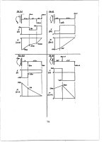
2. Develop the two-dimensional form of the Cartesian equilibrium equations by drawing a
free-body diagram of an infinitesimal section:
5
Prob. 2
3. Use the free body diagram of the previous problem to show that τ
xy
= τ
yx
.
4. Use a free-body diagram approach to show that in polar coordinates the equilibrium equa-
tions are
∂σ
r
∂r
+
1

r
∂τ
rθ
∂θ
+
σ
r
− σ
θ
r
=0
∂τ
rθ
∂r
+
1
r
∂σ
θ
∂θ
+2
τ
rθ
r
=0
5. Develop the above equations for equilibrium in polar coordinates by transforming the
Cartesian equations using
x = r cos θ
y = r sin θ
6. The Airy stress function φ(x, y) is defined such that the Cartesian Cauchy stresses are

σ
x
=
∂
2
φ
∂y
2
,σ
y
=
∂
2
φ
∂x
2
,τ
xy
= −
∂
2
φ
∂x∂y
Show that the stresses obtained from this procedure satisfy the equilibrium equations.
6
Transformation of Stresses and Strains
David Roylance
Department of Materials Science and Engineering
Massachusetts Institute of Technology
Cambridge, MA 02139

May 14, 2001
Introduction
One of the most common problems in mechanics of materials involves transformation of axes.
For instance, we may know the stresses acting on xy planes, but are really more interested in
the stresses acting on planes oriented at, say, 30
◦
to the x axis as seen in Fig. 1, perhaps because
these are close-packed atomic planes on which sliding is prone to occur, or is the angle at which
two pieces of lumber are glued together in a “scarf” joint. We seek a means to transform the
stresses to these new x

y

planes.
Figure 1: Rotation of axes in two dimensions.
These transformations are vital in analyses of stress and strain, both because they are needed
to compute critical values of these entities and also because the tensorial nature of stress and
strain is most clearly seen in their transformation properties. Other entities, such as moment of
inertia and curvature, also transform in a manner similar to stress and strain. All of these are
second-rank tensors, an important concept that will be outlined later in this module.
Direct approach
The rules for stress transformations can be developed directly from considerations of static
equilibrium. For illustration, consider the case of uniaxial tension shown in Fig. 2 in which all
stresses other than σ
y
are zero. A free body diagram is then constructed in which the specimen
is “cut” along the inclined plane on which the stresses, labeled σ
y

and τ

x

y

, are desired. The
key here is to note that the area on which these transformed stresses act is different than the
area normal to the y axis, so that both the areas and the forces acting on them need to be
“transformed.” Balancing forces in the y

direction (the direction normal to the inclined plane):
1
Figure 2: An inclined plane in a tensile specimen.
(σ
y
A)cosθ =σ
y


A
cos θ

σ
y

= σ
y
cos
2
θ (1)
Similarly, a force balance in the tangential direction gives

τ
x

y

= σ
y
sin θ cos θ (2)
Example 1
Consider a unidirectionally reinforced composite ply with strengths ˆσ
1
in the fiber direction, ˆσ
2
in the
transverse direction, and ˆτ
12
in shear. As the angle θ between the fiber direction and an applied tensile
stress σ
y
is increased, the stress in the fiber direction will decrease according to Eqn. 1. If the ply were
to fail by fiber fracture alone, the stress σ
y,b
needed to cause failure would increase with misalignment
according to σ
y,b
=ˆσ
1
/cos
2
θ.

However, the shear stresses as given by Eqn. 2 increase with θ,sotheσ
y
stress needed for shear
failure drops. The strength σ
y,b
is the smaller of the stresses needed to cause fiber-direction or shear
failure, so the strength becomes limited by shear after only a few degrees of misalignment. In fact, a 15
◦
off-axis tensile specimen has been proposed as a means of measuring intralaminar shear strength. When
the orientation angle approaches 90
◦
, failure is dominated by the transverse strength. The experimental
data shown in Fig. 3 are for glass-epoxy composites
1
, which show good but not exact agreement with
these simple expressions.
A similar approach, but generalized to include stresses σ
x
and τ
xy
on the original xy planes
as shown in Fig. 4 (see Prob. 2) gives:
σ
x

= σ
x
cos
2
θ + σ

y
sin
2
θ +2τ
xy
sin θ cos θ
σ
y

= σ
x
sin
2
θ + σ
y
cos
2
θ − 2τ
xy
sin θ cos θ
τ
x

y

=(σ
y
−σ
x
)sinθ cos θ + τ

xy
(cos
2
θ − sin
2
θ)
(3)
These relations can be written in pseudovector-matrix form as





σ
x

σ
y

τ
x

y






=




c
2
s
2
2sc
s
2
c
2
−2sc
−sc sc c
2
− s
2








σ
x
σ
y
τ

xy





(4)
1
R.M. Jones, Mechanics of Composite Materials, McGraw-Hill, 1975.
2
Figure 3: Stress applied at an angle to the fibers in a one-dimensional ply.
Figure 4: Stresses on inclined plane.
where c =cosθand s =sinθ. This can be abbreviated as
σ

= Aσ (5)
where A is the transformation matrix in brackets above. This expression would be valid for
three dimensional as well as two dimensional stress states, although the particular form of A
given in Eqn. 4 is valid in two dimensions only (plane stress), and for Cartesian coordinates.
Using either mathematical or geometric arguments (see Probs. 3 and 4), it can be shown
that the components of infinitesimal strain transform by almost the same relations:






x



y

1
2
γ
x

y






= A






x

y
1
2
γ
xy






(6)
The factor of 1/2 on the shear components arises from the classical definition of shear strain,
which is twice the tensorial shear strain. This introduces some awkwardness into the transfor-
mation relations, some of which can be reduced by defining the Reuter’s matrix as
[R]=



100
010
002



or [R]
−1
=



100
010
00
1
2




(7)
We can now write:






x


y

γ
x

y






= R







x


y

1
2
γ
x

y






= RA






x

y
1
2

γ
xy





= RAR
−1






x

y
γ
xy





3
Or


= RAR

−1
 (8)
As can be verified by expanding this relation, the transformation equations for strain can also
be obtained from the stress transformation equations (e.g. Eqn. 3) by replacing σ with  and τ
with γ/2:

x

= 
x
cos
2
θ + 
y
sin
2
θ + γ
xy
sin θ cos θ

y

= 
x
sin
2
θ + 
y
cos
2

θ − γ
xy
sin θ cos θ
γ
x

y

=2(
y
−
x
)sinθ cos θ + γ
xy
(cos
2
θ − sin
2
θ)
(9)
Example 2
Consider the biaxial strain state
 =




x



y

γ
x

y




=



0.01
−0.01
0



The state of strain 

referred to axes rotated by θ =45
◦
from the x-y axes can be computed by matrix
multiplication as:
A =


c

2
s
2
2sc
s
2
c
2
−2sc
−sc sc c
2
− s
2


=


0.50.51.0
0.50.5−1.0
−0.50.50.0


Then


= RAR
−1

=



1.00.00.0
0.01.00.0
0.00.02.0




0.50.51.0
0.50.5−1.0
−0.50.50.0




1.00.00.0
0.01.00.0
0.00.00.5


=



0.00
0.00
−0.02




Obviously, the matrix multiplication method is tedious unless matrix-handling software is available, in
which case it becomes very convenient.
Mohr’s circle
Everyday experience with such commonplace occurrences as pushing objects at an angle gives
us all a certain intuitive sense of how vector transformations work. Second-rank tensor trans-
formations seem more abstract at first, and a device to help visualize them is of great value. As
it happens, the transformation equations have a famous (among engineers) graphical interpre-
tation known as Mohr’s circle
2
. The Mohr procedure is justified mathematically by using the
trigonometric double-angle relations to show that Eqns. 3 have a circular representation (see
Prob. 5), but it can probably best be learned simply by memorizing the following recipe
3
:
2
Presented in 1900 by the German engineer Otto Mohr (1835–1918).
3
An interactive web demonstration of Mohr’s circle construction is available at
< />4
1. Draw the stress square, noting the values on the x and y faces; Fig. 5(a) shows a hypo-
thetical case for illustration. For the purpose of Mohr’s circle only, regard a shear stress
acting in a clockwise-rotation sense as being positive, and counter-clockwise as negative.
The shear stresses on the x and y faces must then have opposite signs. The normal stresses
are positive in tension and negative in compression, as usual.
Figure 5: Stress square (a) and Mohr’s circle (b) for σ
x
=+5,σ
y
=−3, τ

xy
= +4. (c) Stress
state on inclined plane.
2. Construct a graph with τ as the ordinate (y axis) and σ as abscissa, and plot the stresses
on the x and y faces of the stress square as two points on this graph. Since the shear
stresses on these two faces are the negative of one another, one of these points will be
above the σ-axis exactly as far as the other is below. It is helpful to label the two points
as x and y.
3. Connect these two points with a straight line. It will cross the σ axis at the line’s midpoint.
This point will be at (σ
x
+ σ
y
)/2, which in our illustration is [5 + (−3)]/2=1.
4. Place the point of a compass at the line’s midpoint, and set the pencil at the end of the
line. Draw a circle with the line as a diameter. The completed circle for our illustrative
stress state is shown in Fig. 5(b).
5. To determine the stresses on a stress square that has been rotated through an angle θ
with respect to the original square, rotate the diametral line inthesamedirectionthrough
twice this angle; i.e. 2θ. The new end points of the line can now be labeled x

and y

,and
their σ-τ values are the stresses on the rotated x

-y

axes as shown in Fig. 5(c).
There is nothing mysterious or magical about the Mohr’s circle; it is simply a device to help

visualize how stresses and other second-rank tensors change when the axes are rotated.
It is clear in looking at the Mohr’s circle in Fig. 5(c) that there is something special about
axis rotations that cause the diametral line to become either horizontal or vertical. In the first
case, the normal stresses assume maximal values and the shear stresses are zero. These normal
stresses are known as the principal stresses, σ
p1
and σ
p2
, and the planes on which they act are
the principal planes. If the material is prone to fail by tensile cracking, it will do so by cracking
along the principal planes when the value of σ
p1
exceeds the tensile strength.
Example 3
It is instructive to use a Mohr’s circle construction to predict how a piece of blackboard chalk will break
in torsion, and then verify it in practice. The torsion produces a state of pure shear as shown in Fig. 6,
5
which causes the principal planes to appear at ±45
◦
to the chalk’s long axis. The crack will appear
transverse to the principal tensile stress, producing a spiral-like failure surface. (As the crack progresses
into the chalk, the state of pure shear is replaced by a more complicated stress distribution, so the last
part of the failure surface deviates from this ideal path to one running along the axial direction.) This
is the same type of fracture that occurred all too often in skiers’ femurs, before the advent of modern
safety bindings.
Figure 6: Mohr’s circle for simple torsion.
Figure 7: Principal stresses on Mohr’s circle.
By direct Pythagorean construction as shown in Fig. 7, the Mohr’s circle shows that the
angle from the x-y axes to the principal planes is
tan 2θ

p
=
τ
xy
(σ
x
− σ
y
)/2
(10)
and the values of the principal stresses are
σ
p1,p1
=
σ
x
+ σ
y
2
±


σ
x
− σ
y
2

2
+ τ

2
xy
(11)
where the first term above is the σ-coordinate of the circle’s center, and the second is its radius.
When the Mohr’s circle diametral line is vertical, the shear stresses become maximum, equal
in magnitude to the radius of the circle:
6
τ
max
=


σ
x
− σ
y
2

2
+ τ
2
xy
=
σ
p1
− σ
p2
2
(12)
The points of maximum shear are 90

◦
away from the principal stress points on the Mohr’s circle,
so on the actual specimen the planes of maximum shear are 45
◦
from the principal planes. The
molecular sliding associated with yield is driven by shear, and usually takes place on the planes
of maximum shear. A tensile specimen has principal planes along and transverse to its loading
direction, so shear slippage will occur on planes ±45
◦
from the loading direction. These slip
planes can often be observed as “shear bands” on the specimen.
Note that normal stresses may appear on the planes of maximum shear, so the situation
is not quite the converse of the principal planes, on which the shear stresses vanish while the
normal stresses are maximum. If the normal stresses happen to vanish on the planes of maximum
shear, the stress state is said to be one of “pure shear,” such as is induced by simple torsion.
A state of pure shear is therefore one for which a rotation of axes exists such that the normal
stresses vanish, which is possible only if the center of the Mohr’s circle is at the origin, i.e.
(σ
x
+ σ
y
)/2 = 0. More generally, a state of pure shear is one in which the trace of the stress
(and strain) matrix vanishes.
Example 4
Figure 8: Strain and stress Mohr’s circles for simple shear.
Mohr’s circles can be drawn for strains as well as stresses, with shear strain plotted on the ordinate and
normal strain on the abscissa. However, the ordinate must be γ/2 rather than just γ, due to the way
classical infinitesimal strains are defined. Consider a state of pure shear with strain γ and stress τ as
shown in Fig. 8, such as might be produced by placing a circular shaft in torsion. A Mohr’s circle for
strain quickly shows the principal strain, on a plane 45

◦
away, is given by 
1
= γ/2. Hooke’s law for shear
gives τ = Gγ,so
1
=τ/2G. The principal strain is also related to the principal stresses by

1
=
1
E
(σ
1
− νσ
2
)
The Mohr’s circle for stress gives σ
1
= −σ
2
= τ, so this can be written
τ
2G
=
1
E
[τ − ν(−τ)]
Canceling τ and rearranging, we have the relation among elastic constants stated earlier without proof:
G =

E
2(1 + ν)
7
General approach
Figure 9: Transformation of vectors.
Another approach to the stress transformation equations, capable of easy extension to three
dimensions, starts with the familiar relations by which vectors are transformed in two dimensions
(see Fig. 9):
T
x

= T
x
cos θ + T
y
sin θ
T
y

= −T
x
sin θ + T
y
cos θ
In matrix form, this is

T
x

T

y


=

cos θ sin θ
− sin θ cos θ

T
x
T
y

or
T

= aT (13)
where a is another transformation matrix that serves to transform the vector components in the
original coordinate system to those in the primed system. In index-notation terms, this could
also be denoted a
ij
,sothat
T

i
=a
ij
T
j
The individual elements of a

ij
are the cosines of the angles between the i
th
primed axis and the
j
th
unprimed axis.
It can be shown by direct examination that the a matrix has the useful property that its
inverse equals its transpose; i.e., a
−1
= a
T
. We can multiply Eqn. 13 by a
T
to give
a
T
T

=(a
T
a)T=T (14)
so the transformation can go from primed to unprimed, or the reverse.
These relations can be extended to yield an expression for transformation of stresses (or
strains, or moments of inertia, or other similar quantities). Recall Cauchy’s relation in matrix
form:
[σ]ˆn = T
UsingEqn.14totransformtheˆnand T vectors into their primed counterparts, we have
8
[σ]a

T
ˆn

= a
T
T

Multiplying through by a:
(a[σ]a
T
)ˆn

=(aa
T
)T

= T

This is just Cauchy’s relation again, but in the primed coordinate frame. The quantity in
parentheses must therefore be [σ

]:
[σ

]=a[σ]a
T
(15)
Therefore, transformation of stresses and can be done by pre- and postmultiplying by the same
transformation matrix applicable to vector transformation. This can also be written out using
index notation, which provides another illustration of the transformation differences between

scalars (zero-rank tensors), vectors (first-rank tensors), and second-rank tensors:
rank 0: b

= b
rank 1: T

i
= a
ij
T
j
rank 2: σ

ij
= a
ij
a
kl
σ
kl
(16)
In practical work, it is not always a simple matter to write down the nine elements of the
a matrix needed in Eqn. 15. The squares of the components of ˆn for any given plane must
sum to unity, and in order for the three planes of the transformed stress cube to be mutually
perpendicular the dot product between any two plane normals must vanish. So not just any nine
numbers will make sense. Obtaining a is made much easier by using “Euler angles” to describe
axis transformations in three dimensions.
Figure 10: Transformation in terms of Euler angles.
As shown in Fig. 10, the final transformed axes are visualized as being achieved in three
steps: first, rotate the original x-y-z axes by an angle ψ (psi) around the z-axis to obtain a

new frame we may call x

-y

-z. Next, rotate this new frame by an angle θ about the x

axis to
obtain another frame we can call x

-y

-z

. Finally, rotate this frame by an angle φ (phi) around
the z

axis to obtain the final frame x

-y

-z

. These three transformations correspond to the
transformation matrix
a =


cos ψ sin ψ 0
− sin ψ cos ψ 0
001





10 0
0cosθsin θ
0 − sin θ cos θ




cos φ sin φ 0
− sin φ cos φ 0
001


9
This multiplication would certainly be a pain if done manually, but is a natural for a computa-
tional approach.
Example 5
The output below shows a computer evaluation of a three-dimensional stress transformation, in this
case using Maple
TM
symbolic mathematics software.
# read linear algebra library
> with(linalg):
# Define Euler-angle transformation matrices:
> a1:=array(1 3,1 3,[[cos(psi),sin(psi),0],[-sin(psi),cos(psi),0],[0,0
> ,1]]);
[cos(psi) sin(psi) 0]

a1 := [-sin(psi) cos(psi) 0]
[0 0 1]
> a2:=array(1 3,1 3,[[1,0,0],[0,cos(theta),sin(theta)],[0,-sin(theta),
> cos(theta)]]);
[1 0 0 ]
a2 := [0 cos(theta) sin(theta)]
[0 -sin(theta) cos(theta)]
> a3:=array(1 3,1 3,[[cos(phi),sin(phi),0],[-sin(phi),cos(phi),0],[0,0
> ,1]]);
[cos(phi) sin(phi) 0]
a3 := [-sin(phi) cos(phi) 0]
[0 0 1]
# Overall transformation matrix (multiply individual Euler matrices):
> a:=a1&*a2&*a3;
a := (a1 &* a2) &* a3
# Set precision and read in Euler angles (converted to radians); here
# we are rotating 30 degrees around the z axis only.
> Digits:=4;psi:=0;theta:=30*(Pi/180);phi:=0;
Digits := 4
psi := 0
theta := 1/6 Pi
phi := 0
# Display transformation matrix for these angles: "evalf" evaluates the
# matrix element, and "map" applies the evaluation to each element of
# the matrix.
> aa:=map(evalf,evalm(a));
[1. 0. 0. ]
aa := [0. .8660 .5000]
[0. 5000 .8660]
# Define the stress matrix in the unprimed frame:

> sigma:=array(1 3,1 3,[[1,2,3],[2,4,5],[3,5,6]]);
[1 2 3]
sigma := [2 4 5]
[3 5 6]
# The stress matrix in the primed frame is then given by Eqn. 15:
> ’sigma_prime’=map(evalf,evalm(aa&*sigma&*transpose(aa)));
[ 1. 3.232 1.598]
sigma_prime = [3.232 8.830 3.366]
[1.598 3.366 1.170]
10
Principal stresses and planes in three dimensions
Figure 11: Traction vector normal to principal plane.
The Mohr’s circle procedure is not capable of finding principal stresses for three-dimensional
stress states, and a more general method is needed. In three dimensions, we seek orientations
of axes such that no shear stresses appear, leaving only normal stresses in three orthogonal
directions. The vanishing of shear stresses on a plane means that the stress vector T is normal
to the plane, illustrated in two dimensions in Fig. 11. The traction vector can therefore be
written as
T = σ
p
ˆ
n
where σ
p
is a simple scalar quantity, the magnitude of the stress vector. Using this in Cauchy’s
relation:
σ ˆn = T = σ
p
ˆn
(σ − σ

p
I) ˆn = 0 (17)
Here I is the unit matrix. This system will have a nontrivial solution (ˆn = 0)onlyifits
determinant is zero:
|σ − σ
p
I| =







σ
x
− σ
p
τ
xy
τ
xz
τ
xy
σ
y
− σ
p
τ
yz

τ
xz
τ
yz
σ
z
− σ
p







= 0
Expanding the determinant yields a cubic polynomial equation in σ
p
:
f(σ
p
)=σ
3
p
−I
1
σ
2
p
+I

2
σ
p
−I
3
= 0 (18)
This is the characteristic equation for stress, where the coefficients are
I
1
= σ
x
+ σ
y
+ σ
z
= σ
kk
(19)
I
2
= σ
x
σ
y
+ σ
x
σ
z
+ σ
y

σ
z
− τ
2
xy
− τ
2
yz
− τ
2
xz
=
1
2
(σ
ii
σ
jj
− σ
ij
σ
ij
) (20)
11
I
3
=det|σ|=
1
3
σ

ij
σ
jk
σ
ki
(21)
These I parameters are known as the invariants of the stress state; they do not change with
transformation of the coordinates and can be used to characterize the overall nature of the
stress. For instance I
1
, which has been identified earlier as the trace of the stress matrix, will be
seen in a later section to be a measure of the tendency of the stress state to induce hydrostatic
dilation or compression. We have already noted that the stress state is one of pure shear if its
trace vanishes.
Since the characteristic equation is cubic in σ
p
, it will have three roots, and it can be shown
that all three roots must be real. These roots are just the principal stresses σ
p1
, σ
p2
,andσ
p3
.
Example 6
Consider a state of simple shear with τ
xy
= 1 and all other stresses zero:
[σ]=



010
100
000


The invariants are
I
1
=0,I
2
=−1,I
3
=0
and the characteristic equation is
σ
3
p
− σ
p
=0
This equation has roots of (-1,0,1) corresponding to principal stresses σ
p1
=1,σ
p2
=0,σ
p3
=−1,
and is plotted in Fig. 12. This is the same stress state considered in Example 4, and the roots of the
characteristic equation agree with the principal values shown by the Mohr’s circle.

Figure 12: The characteristic equation for τ
xy
= 1, all other stresses zero.
12
Problems
1. Develop an expression for the stress needed to cause transverse failure in a unidirectionally
oriented composite as a function of the angle between the load direction and the fiber
direction, and show this function in a plot of strength versus θ.
2. Use a free-body force balance to derive the two-dimensional Cartesian stress transformation
equations as
σ
x

= σ
x
cos
2
θ + σ
y
sin
2
θ +2τ
xy
sin θ cos θ
σ
y

= σ
x
sin

2
θ + σ
y
cos
2
θ − 2τ
xy
sin θ cos θ
τ
x

y

=(σ
y
−σ
x
)sinθ cos θ + τ
xy
(cos
2
θ − sin
2
θ)
Or






σ
x

σ
y

τ
x

y






=



c
2
s
2
2sc
s
2
c
2
−2sc

−sc sc c
2
− s
2








σ
x
σ
y
τ
xy





where c =cosθand s =sinθ.
Prob. 2
3. Develop mathematical relations for displacements and gradients along transformed axes
of the form
u

= u cos θ + v sin θ

∂
∂x

=
∂
∂x
·
∂x
∂x

+
∂
∂y
·
∂y
∂x

=
∂
∂x
· cos θ +
∂
∂y
· sin θ
with analogous expressions for v

and ∂/∂y

. Use these to obtain the strain transformation
equations (Eqn. 6).

4. Consider a line segment AB of length ds
2
= dx
2
+ dy
2
, oriented at an angle θ from the
Cartesian x − y axes as shown. Let the differential displacement of end B relative to end
A be
du =
∂u
∂x
dx +
∂u
∂y
dy
13
dv =
∂v
∂x
dx +
∂v
∂y
dy
Use this geometry to derive the strain transformation equations (Eqn. 6), where the x

axis is along line AB.
Prob. 4
5. Employ double-angle trigonometric relations to show that the two-dimensional Cartesian
stress transformation equations can be written in the form

σ
x

=
σ
x
+σ
y
2
+
σ
x
−σ
y
2
cos 2θ + τ
xy
sin 2θ
τ
x

y

= −
σ
x
−σ
y
2
sin 2θ + τ

xy
cos 2θ
σ
y

=
σ
x
+σ
y
2
+
σ
x
−σ
y
2
cos 2θ − τ
xy
sin 2θ
Use these relations to justify the Mohr’s circle construction.
6. Use matrix multiplication (Eqns. 5 or 8) to transform the following stress and strain states
to axes rotated by θ =30
◦
from the original x-y axes.
(a)
σ =






1.0
−2.0
3.0





(b)
 =





0.01
−0.02
0.03





7. Sketch the Mohr’s circles for each of the stress states shown in the figure below.
8. Construct Mohr’s circle solutions for the transformations of Prob. 6.
9. Draw the Mohr’s circles and determine the magnitudes of the principal stresses for the
following stress states. Denote the principal stress state on a suitably rotated stress square.
(a) σ

x
=30MPa,σ
y
=−10 MPa, τ
xy
=25MPa.
(b) σ
x
= −30 MPa, σ
y
= −90 MPa, τ
xy
= −40 MPa.
(c) σ
x
= −10 MPa, σ
y
=20MPa,τ
xy
= −15 MPa.
14
Prob. 7
10. Show that the values of principal stresses given by Mohr’s circle agree with those ob-
tained mathematically by setting to zero the derivatives of the stress with respect to the
transformation angle.
11. For the 3-dimensional stress state σ
x
= 25, σ
y
= −15, σ

z
= −30, τ
yz
= 20, τ
xz
= 10,
τ
xy
=30(allinMPa):
(a) Determine the stress state for Euler angles ψ =20
◦
,θ=30
◦
,φ=25
◦
.
(b) Plot the characteristic equation.
(c) Determine the principal stresses.
15