david roylance mechanics of materials Part 2 pdf
Bạn đang xem bản rút gọn của tài liệu. Xem và tải ngay bản đầy đủ của tài liệu tại đây (471.93 KB, 25 trang )
U = −
(n − 1)ACe
2
nr
0
where A is the Madelung constant, C is the appropriate units conversion factor, and e is
the ionic charge.
3. Measurements of bulk compressibility are valuable for probing the bond energy function,
because unlike simple tension, hydrostatic pressure causes the interionic distance to de-
crease uniformly. The modulus of compressibility K of a solid is the ratio of the pressure
p needed to induce a relative change in volume dV/V :
K = −
dp
(dV )/V
The minus sign is needed because positive pressures induce reduced volumes (volume
change negative).
(a) Use the relation dU = pdV for the energy associated with pressure acting through a
small volume change to show
K
V
0
=
d
2
U
dV
2
V =V
0
where V
0
is the crystal volume at the equilibrium interionic spacing r = a
0
.
(b) The volume of an ionic crystal containing N negative and N positive ions can be
written as V = cNr
3
where c is a constant dependent on the type of lattice (2 for NaCl).
Use this to obtain the relation
K
V
0
=
d
2
U
dV
2
V =V
0
=
1
9c
2
N
2
r
2
·
d
dr
1
r
2
dU
dr
(c) Carry out the indicated differentiation of the expression for binding energy to obtain
the expression
K
V
0
=
K
cNr
3
0
=
N
9c
2
Nr
2
0
−4ACe
r
5
0
+
n(n +3)B
r
n+4
0
Then using the expression B = ACe
2
r
n−1
0
/n, obtain the formula for n in terms of com-
pressibility:
n =1+
9cr
4
0
K
ACe
2
4. Complete the spreadsheet below, filling in the values for repulsion exponent n and lattice
energy U.
16
type r
0
(pm) K (GPa) A n U(kJ/mol) U
expt
LiF 201.4 6.710e+01 1.750 -1014
NaCl 282.0 2.400e+01 1.750 -764
KBr 329.8 1.480e+01 1.750 -663
The column labeled U
expt
lists experimentally obtained values of the lattice energy.
5. Given the definition of Helmholtz free energy:
A = U − TS
along with the first and second laws of thermodynamics:
dU = dQ + dW
dQ = TdS
where U is the internal energy, T is the temperature, S is the entropy, Q is the heat and
W is the mechanical work, show that the force F required to hold the ends of a tensile
specimen a length L apart is related to the Helmholtz energy as
F =
∂A
∂L
T,V
6. Show that the temperature dependence of the force needed to hold a tensile specimen at
fixed length as the temperature is changed (neglecting thermal expansion effects) is related
to the dependence of the entropy on extension as
∂F
∂T
L
= −
∂S
∂L
T
7. (a) Show that if an ideal rubber (dU =0)ofmassMand specific heat c is extended
adiabatically, its temperature will change according to the relation
∂T
∂L
=
−T
Mc
∂S
∂L
i.e. if the entropy is reduced upon extension, the temperature will rise. This is known as
the thermoelastic effect.
(b) Use this expression to obtain the temperature change dT in terms of an increase dλ in
the extension ratio as
dT =
σ
ρc
dλ
where σ is the engineering stress (load divided by original area) and ρ is the mass density.
8. Show that the end-to-end distance r
0
of a chain composed of n freely-jointed links of length
a is given by r
o
= na
2
.
17
9. Evalute the temperature rise in a rubber specimen of ρ = 1100 kg/m
3
, c = 2 kJ/kg·K,
NkT = 500 kPa, subjected to an axial extension λ =4.
10. Show that the initial engineering modulus of a rubber whose stress-strain curve is given
by Eqn. 14 is E =3NRT.
11. Calculate the Young’s modulus of a rubber of density 1100 gm/mol and whose inter-
crosslink segments have a molecular weight of 2500 gm/mol. The temperature is 25
◦
C.
12. Show that in the case of biaxial extension (λ
x
and λ
y
prescribed), the x-direction stress
based on the original cross-sectional dimensions is
σ
x
= NkT
λ
x
−
1
λ
3
x
λ
2
y
and based on the deformed dimensions
t
σ
x
= NkT
λ
2
x
−
1
λ
2
x
λ
2
y
where the t subscript indicates a “true” or current stress.
13. Estimate the initial elastic modulus E, at a temperature of 20C, of an elastomer having a
molecular weight of 7,500 gm/mol between crosslinks and a density of 1.0 gm/cm
3
.What
is the percentage change in the modulus if the temperature is raised to 40C?
14. Consider a line on a rubber sheet, originally oriented at an angle φ
0
from the vertical.
When the sheet is stretched in the vertical direction by an amount λ
y
= λ, the line rotates
to a new inclination angle φ
. Show that
tan φ
=
1
λ
3/2
tan φ
0
15. Before stretching, the molecular segments in a rubber sheet are assumed to be distributed
uniformly over all directions, so the the fraction of segments f(φ) oriented in a particular
range of angles dφ is
f(φ)=
dA
A
=
2πr
2
sin φdφ
2πr
18
The Herrman orientation parameter is defined in terms of the mean orientation as
f =
1
2
3cos
2
φ
−1
, cos
2
φ
=
π/2
0
cos
2
φ
f(φ) dφ
Using the result of the previous problem, plot the orientation function f as a function of
the extension ratio λ.
19
INTRODUCTION TO COMPOSITE MATERIALS
David Roylance
Department of Materials Science and Engineering
Massachusetts Institute of Technology
Cambridge, MA 02139
March 24, 2000
Introduction
This module introduces basic concepts of stiffness and strength underlying the mechanics of
fiber-reinforced advanced composite materials. This aspect of composite materials technology
is sometimes terms “micromechanics,” because it deals with the relations between macroscopic
engineering properties and the microscopic distribution of the material’s constituents, namely
the volume fraction of fiber. This module will deal primarily with unidirectionally-reinforced
continuous-fiber composites, and with properties measured along and transverse to the fiber
direction.
Materials
The term comp osite could mean almost anything if taken at face value, since all materials are
composed of dissimilar subunits if examined at close enough detail. But in modern materials
engineering, the term usually refers to a “matrix” material that is reinforced with fibers. For in-
stance, the term “FRP” (for Fiber Reinforced Plastic) usually indicates a thermosetting polyester
matrix containing glass fibers, and this particular composite has the lion’s share of today’s
commercial market. Figure 1 shows a laminate fabricated by “crossplying” unidirectionally-
reinforced layers in a 0
◦
-90
◦
stacking sequence.
Many composites used today are at the leading edge of materials technology, with perfor-
mance and costs appropriate to ultrademanding applications such as spacecraft. But heteroge-
neous materials combining the best aspects of dissimilar constituents have been used by nature
for millions of years. Ancient society, imitating nature, used this approach as well: the Book of
Exodus speaks of using straw to reinforce mud in brickmaking, without which the bricks would
have almost no strength.
As seen in Table 1
1
, the fibers used in modern composites have strengths and stiffnesses
far above those of traditional bulk materials. The high strengths of the glass fibers are due to
processing that avoids the internal or surface flaws which normally weaken glass, and the strength
and stiffness of the polymeric aramid fiber is a consequence of the nearly perfect alignment of
the molecular chains with the fiber axis.
1
F.P. Gerstle, “Composites,” Encyclopedia of Polymer Science and Engineering, Wiley, New York, 1991. Here
E is Young’s modulus, σ
b
is breaking stress,
b
is breaking strain, and ρ is density.
1
Figure 1: A crossplied FRP laminate, showing nonuniform fiber packing and microcracking
(from Harris, 1986).
Table 1: Properties of Composite Reinforcing Fibers.
Material Eσ
b
b
ρE/ρσ
b
/ρ cost
(GPa) (GPa) (%) (Mg/m
3
) (MJ/kg) (MJ/kg) ($/kg)
E-glass 72.4 2.4 2.6 2.54 28.5 0.95 1.1
S-glass 85.5 4.5 2.0 2.49 34.3 1.8 22–33
aramid 124 3.6 2.3 1.45 86 2.5 22–33
boron 400 3.5 1.0 2.45 163 1.43 330–440
HS graphite 253 4.5 1.1 1.80 140 2.5 66–110
HM graphite 520 2.4 0.6 1.85 281 1.3 220–660
Of course, these materials are not generally usable as fibers alone, and typically they are
impregnated by a matrix material that acts to transfer loads to the fibers, and also to pro-
tect the fibers from abrasion and environmental attack. The matrix dilutes the properties to
some degree, but even so very high specific (weight-adjusted) properties are available from these
materials. Metal and glass are available as matrix materials, but these are currently very ex-
pensive and largely restricted to R&D laboratories. Polymers are much more commonly used,
with unsaturated styrene-hardened polyesters having the majority of low-to-medium perfor-
mance applications and epoxy or more sophisticated thermosets having the higher end of the
market. Thermoplastic matrix composites are increasingly attractive materials, with processing
difficulties being perhaps their principal limitation.
Stiffness
The fibers may be oriented randomly within the material, but it is also possible to arrange for
them to be oriented preferentially in the direction expected to have the highest stresses. Such
a material is said to be anisotropic (different properties in different directions), and control of
the anisotropy is an important means of optimizing the material for specific applications. At
a microscopic level, the properties of these composites are determined by the orientation and
2
distribution of the fibers, as well as by the properties of the fiber and matrix materials. The
topic known as composite micromechanics is concerned with developing estimates of the overall
material properties from these parameters.
Figure 2: Loading parallel to the fibers.
Consider a typical region of material of unit dimensions, containing a volume fraction V
f
of
fibers all oriented in a single direction. The matrix volume fraction is then V
m
=1−V
f
.This
region can be idealized as shown in Fig. 2 by gathering all the fibers together, leaving the matrix
to occupy the remaining volume — this is sometimes called the “slab model.” If a stress σ
1
is
applied along the fiber direction, the fiber and matrix phases act in parallel to support the load.
In these parallel connections the strains in each phase must be the same, so the strain
1
in the
fiber direction can be written as:
f
=
m
=
1
The forces in each phase must add to balance the total load on the material. Since the forces in
each phase are the phase stresses times the area (here numerically equal to the volume fraction),
we have
σ
1
= σ
f
V
f
+ σ
m
V
m
= E
f
1
V
f
+ E
m
1
V
m
The stiffness in the fiber direction is found by dividing by the strain:
E
1
=
σ
1
1
= V
f
E
f
+ V
m
E
m
(1)
This relation is known as a rule of mixtures prediction of the overall modulus in terms of the
moduli of the constituent phases and their volume fractions.
If the stress is applied in the direction transverse to the fibers as depicted in Fig. 3, the slab
model can be applied with the fiber and matrix materials acting in series. In this case the stress
in the fiber and matrix are equal (an idealization), but the deflections add to give the overall
transverse deflection. In this case it can be shown (see Prob. 5)
1
E
2
=
V
f
E
f
+
V
m
E
m
(2)
Figure 4 shows the functional form of the parallel (Eqn. 1) and series (Eqn. 2) predictions for
the fiber- and transverse-direction moduli.
The prediction of transverse modulus given by the series slab model (Eqn. 2) is considered
unreliable, in spite of its occasional agreement with experiment. Among other deficiencies the
3
Figure 3: Loading perpendicular to the fibers.
assumption of uniform matrix strain being untenable; both analytical and experimental studies
have shown substantial nonuniformity in the matirx strain. Figure 5 shows the photoelastic
fringes in the matrix caused by the perturbing effect of the stiffer fibers. (A more complete
description of these phtoelasticity can be found in the Module on Experimental Strain Analysis,
but this figure can be interpreted simply by noting that closely-spaced photoelastic fringes are
indicative of large strain gradients.
In more complicated composites, for instance those with fibers in more than one direction
or those having particulate or other nonfibrous reinforcements, Eqn. 1 provides an upper bound
to the composite modulus, while Eqn. 2 is a lower bound (see Fig. 4). Most practical cases
will be somewhere between these two values, and the search for reasonable models for these
intermediate cases has occupied considerable attention in the composites research community.
Perhaps the most popular model is an empirical one known as the Halpin-Tsai equation
2
,which
can be written in the form:
E =
E
m
[E
f
+ ξ(V
f
E
f
+ V
m
E
m
)]
V
f
E
m
+ V
m
E
f
+ ξE
m
(3)
Here ξ is an adjustable parameter that results in series coupling for ξ = 0 and parallel averaging
for very large ξ.
Strength
Rule of mixtures estimates for strength proceed along lines similar to those for stiffness. For
instance, consider a unidirectionally reinforced composite that is strained up to the value at
which the fibers begin to break. Denoting this value
fb
, the stress transmitted by the composite
is given by multiplying the stiffness (Eqn. 1):
σ
b
=
fb
E
1
= V
f
σ
fb
+(1−V
f
)σ
∗
The stress σ
∗
is the stress in the matrix, which is given by
fb
E
m
. This relation is linear in V
f
,
rising from σ
∗
to the fiber breaking strength σ
fb
= E
f
fb
. However, this relation is not realistic
at low fiber concentration, since the breaking strain of the matrix
mb
is usually substantially
greater than
fb
. If the matrix had no fibers in it, it would fail at a stress σ
mb
= E
m
mb
.Ifthe
fibers were considered to carry no load at all, having broken at =
fb
and leaving the matrix
2
c.f. J.C Halpin and J.L. Kardos, Polymer Engineering and Science, Vol. 16, May 1976, pp. 344–352.
4
Figure 4: Rule-of-mixtures predictions for longitudinal (E
1
) and transverse (E
2
) modulus, for
glass-polyester composite (E
f
=73.7MPa,E
m
= 4 GPa). Experimental data taken from Hull
(1996).
to carry the remaining load, the strength of the composite would fall off with fiber fraction
according to
σ
b
=(1−V
f
)σ
mb
Since the breaking strength actually observed in the composite is the greater of these two
expressions, there will be a range of fiber fraction in which the composite is weakened by the
addition of fibers. These relations are depicted in Fig. 6.
References
1. Ashton, J.E., J.C. Halpin and P.H. Petit, Primer on Composite Materials: Analysis,Technomic
Press, Westport, CT, 1969.
2. , Harris, B., Engineering Composite Materials, The Institute of Metals, London, 1986.
3. Hull, D. and T.W. Clyne, An Introduction to Composites Materials, Cambridge University
Press, 1996.
4. Jones, R.M., Mechanics of Composite Materials, McGraw-Hill, New York, 1975.
5. Powell, P.C, Engineering with Polymers, Chapman and Hall, London, 1983.
6. Roylance, D., Mechanics o f Materials, Wiley & Sons, New York, 1996.
5
Figure 5: Photoelastic (isochromatic) fringes in a composite model subjected to transverse
tension (from Hull, 1996).
Figure 6: Strength of unidirectional composite in fiber direction.
Problems
1. Compute the longitudinal and transverse stiffness (E
1
,E
2
) of an S-glass epoxy lamina for
a fiber volume fraction V
f
=0.7, using the fiber properties from Table 1, and matrix
properties from the Module on Materials Properties.
2. Plot the longitudinal stiffness E
1
of an E-glass/nylon unidirectionally-reinforced composite,
as a function of the volume fraction V
f
.
3. Plot the longitudinal tensile strength of a E-glass/epoxy unidirectionally-reinforced com-
posite, as a function of the volume fraction V
f
.
4. What is the maximum fiber volume fraction V
f
that could be obtained in a unidirectionally
reinforced with optimal fiber packing?
5. Using the slab model and assuming uniform strain in the matrix, show the transverse
modulus of a unidirectionally-reinforced composite to be
6
1
E
2
=
V
f
E
f
+
V
m
E
m
or in terms of compliances
C
2
= C
f
V
f
+ C
m
V
m
7
STRESS-STRAIN CURVES
David Roylance
Department of Materials Science and Engineering
Massachusetts Institute of Technology
Cambridge, MA 02139
August 23, 2001
Introduction
Stress-strain curves are an extremely important graphical measure of a material’s mechanical
properties, and all students of Mechanics of Materials will encounter them often. However, they
are not without some subtlety, especially in the case of ductile materials that can undergo sub-
stantial geometrical change during testing. This module will provide an introductory discussion
of several points needed to interpret these curves, and in doing so will also provide a preliminary
overview of several aspects of a material’s mechanical properties. However, this module will
not attempt to survey the broad range of stress-strain curves exhibited by modern engineering
materials (the atlas by Boyer cited in the References section can be consulted for this). Several
of the topics mentioned here — especially yield and fracture — will appear with more detail in
later modules.
“Engineering” Stress-Strain Curves
Perhaps the most important test of a material’s mechanical response is the tensile test
1
,inwhich
one end of a rod or wire specimen is clamped in a loading frame and the other subjected to
a controlled displacement δ (see Fig. 1). A transducer connected in series with the specimen
provides an electronic reading of the load P (δ) corresponding to the displacement. Alternatively,
modern servo-controlled testing machines permit using load rather than displacement as the
controlled variable, in which case the displacement δ(P ) would be monitored as a function of
load.
The engineering measures of stress and strain, denoted in this module as σ
e
and
e
respec-
tively, are determined from the measured the load and deflection using the original specimen
cross-sectional area A
0
and length L
0
as
σ
e
=
P
A
0
,
e
=
δ
L
0
(1)
When the stress σ
e
is plotted against the strain
e
,anengineering stress-strain curve such as
that shown in Fig. 2 is obtained.
1
Stress-strain testing, as well as almost all experimental procedures in mechanics of materials, is detailed by
standards-setting organizations, notably the American Society for Testing and Materials (ASTM). Tensile testing
of metals is prescribed by ASTM Test E8, plastics by ASTM D638, and composite materials by ASTM D3039.
1
Figure 1: The tension test.
Figure 2: Low-strain region of the engineering stress-strain curve for annealed polycrystaline
copper; this curve is typical of that of many ductile metals.
In the early (low strain) portion of the curve, many materials obey Hooke’s law to a reason-
able approximation, so that stress is proportional to strain with the constant of proportionality
being the modulus of elasticity or Young’s modulus, denoted E:
σ
e
= E
e
(2)
As strain is increased, many materials eventually deviate from this linear proportionality,
the point of departure being termed the proportional limit. This nonlinearity is usually as-
sociated with stress-induced “plastic” flow in the specimen. Here the material is undergoing
a rearrangement of its internal molecular or microscopic structure, in which atoms are being
moved to new equilibrium positions. This plasticity requires a mechanism for molecular mo-
bility, which in crystalline materials can arise from dislocation motion (discussed further in a
later module.) Materials lacking this mobility, for instance by having internal microstructures
that block dislocation motion, are usually brittle rather than ductile. The stress-strain curve
for brittle materials are typically linear over their full range of strain, eventually terminating in
fracture without appreciable plastic flow.
Note in Fig. 2 that the stress needed to increase the strain beyond the proportional limit
in a ductile material continues to rise beyond the proportional limit; the material requires an
ever-increasing stress to continue straining, a mechanism termed strain hardening.
These microstructural rearrangements associated with plastic flow are usually not reversed
2
when the load is removed, so the proportional limit is often the same as or at least close to the
materials’s elastic limit. Elasticity is the property of complete and immediate recovery from
an imposed displacement on release of the load, and the elastic limit is the value of stress at
which the material experiences a permanent residual strain that is not lost on unloading. The
residual strain induced by a given stress can be determined by drawing an unloading line from
the highest point reached on the se - ee curve at that stress back to the strain axis, drawn with
a slope equal to that of the initial elastic loading line. This is done because the material unloads
elastically, there being no force driving the molecular structure back to its original position.
A closely related term is the yield stress, denoted σ
Y
in these modules; this is the stress
needed to induce plastic deformation in the specimen. Since it is often difficult to pinpoint the
exact stress at which plastic deformation begins, the yield stress is often taken to be the stress
needed to induce a specified amount of permanent strain, typically 0.2%. The construction used
to find this “offset yield stress” is shown in Fig. 2, in which a line of slope E is drawn from the
strain axis at
e
=0.2%; this is the unloading line that would result in the specified permanent
strain. The stress at the point of intersection with the σ
e
−
e
curve is the offset yield stress.
Figure 3 shows the engineering stress-strain curve for copper with an enlarged scale, now
showing strains from zero up to specimen fracture. Here it appears that the rate of strain
hardening
2
diminishes up to a point labeled UTS, for Ultimate Tensile Strength (denoted σ
f
in
these modules). Beyond that point, the material appears to strain soften, so that each increment
of additional strain requires a smaller stress.
Figure 3: Full engineering stress-strain curve for annealed polycrystalline copper.
The apparent change from strain hardening to strain softening is an artifact of the plotting
procedure, however, as is the maximum observed in the curve at the UTS. Beyond the yield
point, molecular flow causes a substantial reduction in the specimen cross-sectional area A,so
thetruestressσ
t
= P/A actually borne by the material is larger than the engineering stress
computed from the original cross-sectional area (σ
e
= P/A
0
). The load must equal the true
stress times the actual area (P = σ
t
A), and as long as strain hardening can increase σ
t
enough
to compensate for the reduced area A, the load and therefore the engineering stress will continue
to rise as the strain increases. Eventually, however, the decrease in area due to flow becomes
larger than the increase in true stress due to strain hardening, and the load begins to fall. This
2
The strain hardening rate is the slope of the stress-strain curve, also called the tangent modulus.
3
is a geometrical effect, and if the true stress rather than the engineering stress were plotted no
maximum would be observed in the curve.
At the UTS the differential of the load P is zero, giving an analytical relation between the
true stress and the area at necking:
P = σ
t
A → dP =0=σ
t
dA + Adσ
t
→−
dA
A
=
dσ
t
σ
t
(3)
The last expression states that the load and therefore the engineering stress will reach a maxi-
mum as a function of strain when the fractional decrease in area becomes equal to the fractional
increase in true stress.
Even though the UTS is perhaps the materials property most commonly reported in tensile
tests, it is not a direct measure of the material due to the influence of geometry as discussed
above, and should be used with caution. The yield stress σ
Y
is usually preferred to the UTS in
designing with ductile metals, although the UTS is a valid design criterion for brittle materials
that do not exhibit these flow-induced reductions in cross-sectional area.
The true stress is not quite uniform throughout the specimen, and there will always be
some location - perhaps a nick or some other defect at the surface - where the local stress is
maximum. Once the maximum in the engineering curve has been reached, the localized flow at
this site cannot be compensated by further strain hardening, so the area there is reduced further.
This increases the local stress even more, which accelerates the flow further. This localized and
increasing flow soon leads to a “neck” in the gage length of the specimen such as that seen in
Fig. 4.
Figure 4: Necking in a tensile specimen.
Until the neck forms, the deformation is essentially uniform throughout the specimen, but
after necking all subsequent deformation takes place in the neck. The neck becomes smaller and
smaller, local true stress increasing all the time, until the specimen fails. This will be the failure
mode for most ductile metals. As the neck shrinks, the nonuniform geometry there alters the
uniaxial stress state to a complex one involving shear components as well as normal stresses.
The specimen often fails finally with a “cup and cone” geometry as seen in Fig. 5, in which
the outer regions fail in shear and the interior in tension. When the specimen fractures, the
engineering strain at break — denoted
f
— will include the deformation in the necked region
and the unnecked region together. Since the true strain in the neck is larger than that in the
unnecked material, the value of
f
will depend on the fraction of the gage length that has necked.
Therefore,
f
is a function of the specimen geometry as well as the material, and thus is only a
4
crude measure of material ductility.
Figure 5: Cup-and-cone fracture in a ductile metal.
Figure 6 shows the engineering stress-strain curve for a semicrystalline thermoplastic. The
response of this material is similar to that of copper seen in Fig. 3, in that it shows a proportional
limit followed by a maximum in the curve at which necking takes place. (It is common to term
this maximum as the yield stress in plastics, although plastic flow has actually begun at earlier
strains.)
Figure 6: Stress-strain curve for polyamide (nylon) thermoplastic.
The polymer, however, differs dramatically from copper in that the neck does not continue
shrinking until the specimen fails. Rather, the material in the neck stretches only to a “natural
draw ratio” which is a function of temperature and specimen processing, beyond which the
material in the neck stops stretching and new material at the neck shoulders necks down. The
neck then propagates until it spans the full gage length of the specimen, a process called drawing.
This process can be observed without the need for a testing machine, by stretching a polyethylene
“six-pack holder,” as seen in Fig. 7.
Not all polymers are able to sustain this drawing process. As will be discussed in the
next section, it occurs when the necking process produces a strengthened microstructure whose
breaking load is greater than that needed to induce necking in the untransformed material just
outside the neck.
5
Figure 7: Necking and drawing in a 6-pack holder.
“True” Stress-Strain Curves
As discussed in the previous section, the engineering stress-strain curve must be interpreted with
caution beyond the elastic limit, since the specimen dimensions experience substantial change
from their original values. Using the true stress σ
t
= P/A rather than the engineering stress
σ
e
= P/A
0
can give a more direct measure of the material’s response in the plastic flow range.
A measure of strain often used in conjunction with the true stress takes the increment of strain
to be the incremental increase in displacement dL divided by the current length L:
d
t
=
dL
l
→
t
=
L
l
0
1
L
dL =ln
L
L
0
(4)
This is called the “true” or “logarithmic” strain.
During yield and the plastic-flow regime following yield, the material flows with negligible
change in volume; increases in length are offset by decreases in cross-sectional area. Prior to
necking, when the strain is still uniform along the specimen length, this volume constraint can
be written:
dV =0→ AL = A
0
L
0
→
L
L
0
=
A
A
0
(5)
The ratio L/L
0
is the extension ratio, denoted as λ. Using these relations, it is easy to develop
relations between true and engineering measures of tensile stress and strain (see Prob. 2):
σ
t
= σ
e
(1 +
e
)=σ
e
λ,
t
=ln(1+
e
)=lnλ (6)
These equations can be used to derive the true stress-strain curve from the engineering curve, up
to the strain at which necking begins. Figure 8 is a replot of Fig. 3, with the true stress-strain
curve computed by this procedure added for comparison.
Beyond necking, the strain is nonuniform in the gage length and to compute the true stress-
strain curve for greater engineering strains would not be meaningful. However, a complete true
stress-strain curve could be drawn if the neck area were monitored throughout the tensile test,
since for logarithmic strain we have
L
L
0
=
A
A
0
→
t
=ln
L
L
0
=ln
A
A
0
(7)
Ductile metals often have true stress-strain relations that can be described by a simple
power-law relation of the form:
6
Figure 8: Comparison of engineering and true stress-strain curves for copper. An arrow indicates
the position on the “true” curve of the UTS on the engineering curve.
σ
t
= A
n
t
→ log σ
t
=logA + n log
t
(8)
Figure 9 is a log-log plot of the true stress-strain data
3
for copper from Fig. 8 that demonstrates
this relation. Here the parameter n =0.474 is called the strain hardening parameter, useful as a
measure of the resistance to necking. Ductile metals at room temperature usually exhibit values
of n from 0.02 to 0.5.
Figure 9: Power-law representation of the plastic stress-strain relation for copper.
A graphical method known as the “Consid`ere construction” uses a form of the true stress-
strain curve to quantify the differences in necking and drawing from material to material. This
method replots the tensile stress-strain curve with true stress σ
t
as the ordinate and extension
ratio λ = L/L
0
as the abscissa. From Eqn. 6, the engineering stress σ
e
corresponding to any
3
Here percent strain was used for
t
; this produces the same value for n but a different A than if full rather
than percentage values were used.
7
valueoftruestressσ
t
is slope of a secant line drawn from origin (λ =0,notλ = 1) to intersect
the σ
t
− λ curve at σ
t
.
Figure 10: Consid`ere construction. (a) True stress-strain curve with no tangents - no necking or
drawing. (b) One tangent - necking but not drawing. (c) Two tangents - necking and drawing.
Among the many possible shapes the true stress-strain curves could assume, let us consider
the concave up, concave down, and sigmoidal shapes shown in Fig. 10. These differ in the
number of tangent points that can be found for the secant line, and produce the following yield
characteristics:
(a) No tangents: Here the curve is always concave upward as in part (a) of Fig. 10, so the
slope of the secant line rises continuously. Therefore the engineering stress rises as well,
without showing a yield drop. Eventually fracture intercedes, so a true stress-strain curve
of this shape identifies a material that fractures before it yields.
(b) One tangent: The curve is concave downward as in part (b) of Fig. 10, so a secant line
reaches a tangent point at λ = λ
Y
. The slope of the secant line, and therefore the
engineering stress as well, begins to fall at this point. This is then the yield stress σ
Y
seen
as a maximum in stress on a conventional stress-strain curve, and λ
Y
is the extension ratio
at yield. The yielding process begins at some adventitious location in the gage length of
the specimen, and continues at that location rather than being initiated elsewhere because
the secant modulus has been reduced at the first location. The specimen is now flowing at
a single location with decreasing resistance, leading eventually to failure. Ductile metals
such as aluminum fail in this way, showing a marked reduction in cross sectional area at
the position of yield and eventual fracture.
(c) Two tangents: For sigmoidal stress-strain curves as in part (c) of Fig. 10, the engineering
stress begins to fall at an extension ration λ
Y
, but then rises again at λ
d
. As in the previous
one-tangent case, material begins to yield at a single position when λ = λ
Y
, producing
a neck that in turn implies a nonuniform distribution of strain along the gage length.
Material at the neck location then stretches to λ
d
, after which the engineering stress there
would have to rise to stretch it further. But this stress is greater than that needed to
stretch material at the edge of the neck from λ
Y
to λ
d
, so material already in the neck
stops stretching and the neck propagates outward from the initial yield location. Only
material within the neck shoulders is being stretched during propagation, with material
inside the necked-down region holding constant at λ
d
, the material’s “natural draw ratio,”
and material outside holding at λ
Y
. When all the material has been drawn into the necked
region, the stress begins to rise uniformly in the specimen until eventually fracture occurs.
The increase in strain hardening rate needed to sustain the drawing process in semicrys-
talline polymers arises from a dramatic transformation in the material’s microstructure. These
materials are initially “spherulitic,” containing flat lamellar crystalline plates, perhaps 10 nm
8
thick, arranged radially outward in a spherical domain. As the induced strain increases, these
spherulites are first deformed in the straining direction. As the strain increases further, the
spherulites are broken apart and the lamellar fragments rearranged with a dominantly axial
molecular orientation to become what is known as the fibrillar microstructure. With the strong
covalent bonds now dominantly lined up in the load-bearing direction, the material exhibits
markedly greater strengths and stiffnesses — by perhaps an order of magnitude — than in the
original material. This structure requires a much higher strain hardening rate for increased
strain, causing the upturn and second tangent in the true stress-strain curve.
Strain energy
The area under the σ
e
−
e
curve up to a given value of strain is the total mechanical energy
per unit volume consumed by the material in straining it to that value. This is easily shown as
follows:
U
∗
=
1
V
PdL=
L
0
P
A
0
dL
L
0
=
0
σd (9)
In the absence of molecular slip and other mechanisms for energy dissipation, this mechanical
energy is stored reversibly within the material as strain energy. When the stresses are low enough
that the material remains in the elastic range, the strain energy is just the triangular area in
Fig. 11:
Figure 11: Strain energy = area under stress-strain curve.
Note that the strain energy increases quadratically with the stress or strain; i.e. that as the
strain increases the energy stored by a given increment of additional strain grows as the square
of the strain. This has important consequences, one example being that an archery bow cannot
be simply a curved piece of wood to work well. A real bow is initially straight, then bent when
it is strung; this stores substantial strain energy in it. When it is bent further on drawing the
arrow back, the energy available to throw the arrow is very much greater than if the bow were
simply carved in a curved shape without actually bending it.
Figure 12 shows schematically the amount of strain energy available for two equal increments
of strain ∆, applied at different levels of existing strain.
The area up to the yield point is termed the modulus of resilience, and the total area up to
fracture is termed the modulus of toughness; these are shown in Fig. 13. The term “modulus”
is used because the units of strain energy per unit volume are N-m/m
3
or N/m
2
, which are the
same as stress or modulus of elasticity. The term “resilience” alludes to the concept that up
to the point of yielding, the material is unaffected by the applied stress and upon unloading
9
Figure 12: Energy associated with increments of strain
Table 1: Energy absorption of various materials.
Material Maximum Maximum Modulus of Density Max. Energy
Strain, % Stress, MPa Toughness, MJ/m
3
kg/m
3
J/kg
Ancient Iron 0.03 70 0.01 7,800 1.3
Modern spring steel 0.3 700 1.0 7,800 130
Yew wood 0.3 120 0.5 600 900
Tendon 8.0 70 2.8 1,100 2,500
Rubber 300 7 10.0 1,200 8,000
will return to its original shape. But when the strain exceeds the yield point, the material is
deformed irreversibly, so that some residual strain will persist even after unloading. The modulus
of resilience is then the quantity of energy the material can absorb without suffering damage.
Similarly, the modulus of toughness is the energy needed to completely fracture the material.
Materials showing good impact resistance are generally those with high moduli of toughness.
Figure 13: Moduli of resilience and toughness.
Table 1
4
lists energy absorption values for a number of common materials. Note that natural
and polymeric materials can provide extremely high energy absorption per unit weight.
During loading, the area under the stress-strain curve is the strain energy per unit volume
absorbed by the material. Conversely, the area under the unloading curve is the energy released
by the material. In the elastic range, these areas are equal and no net energy is absorbed. But
4
J.E. Gordon, Structures, or Why Things Don’t Fall Down, Plenum Press, New York, 1978.
10
if the material is loaded into the plastic range as shown in Fig. 14, the energy absorbed exceeds
the energy released and the difference is dissipated as heat.
Figure 14: Energy loss = area under stress-strain loop.
Compression
The above discussion is concerned primarily with simple tension, i.e. uniaxial loading that
increases the interatomic spacing. However, as long as the loads are sufficiently small (stresses
less than the proportional limit), in many materials the relations outlined above apply equally
well if loads are placed so as to put the specimen in compression rather than tension. The
expression for deformation and a given load δ = PL/AE applies just as in tension, with negative
values for δ and P indicating compression. Further, the modulus E is the same in tension and
compression to a good approximation, and the stress-strain curve simply extends as a straight
line into the third quadrant as shown in Fig. 15.
Figure 15: Stress-strain curve in tension and compression.
There are some practical difficulties in performing stress-strain tests in compression. If
excessively large loads are mistakenly applied in a tensile test, perhaps by wrong settings on the
testing machine, the specimen simply breaks and the test must be repeated with a new specimen.
But in compression, a mistake can easily damage the load cell or other sensitive components,
since even after specimen failure the loads are not necessarily relieved.
Specimens loaded cyclically so as to alternate between tension and compression can exhibit
hysteresis loops if the loads are high enough to induce plastic flow (stresses above the yield
stress). The enclosed area in the loop seen in Fig. 16 is the strain energy per unit volume
released as heat in each loading cycle. This is the well-known tendency of a wire that is being
11
bent back and forth to become quite hot at the region of plastic bending. The temperature of
the specimen will rise according to the magnitude of this internal heat generation and the rate
at which the heat can be removed by conduction within the material and convection from the
specimen surface.
Figure 16: Hysteresis loop.
Specimen failure by cracking is inhibited in compression, since cracks will be closed up rather
than opened by the stress state. A number of important materials are much stronger in com-
pression than in tension for this reason. Concrete, for example, has good compressive strength
and so finds extensive use in construction in which the dominant stresses are compressive. But
it has essentially no strength in tension, as cracks in sidewalks and building foundations attest:
tensile stresses appear as these structures settle, and cracks begin at very low tensile strain in
unreinforced concrete.
References
1. Boyer, H.F., Atlas of Stress-Strain Curves, ASM International, Metals Park, Ohio, 1987.
2. Courtney, T.H., Mechanical Behavior of Materials, McGraw-Hill, New York, 1990.
3. Hayden, H.W., W.G. Moffatt and J. Wulff, The Structure and Properties of Materials:
Vol. III Mechanical Behavior, Wiley, New York, 1965.
Problems
1. The figure below shows the engineering stress-strain curve for pure polycrystalline alu-
minum; the numerical data for this figure are in the file aluminum.txt,whichcanbe
imported into a spreadsheet or other analysis software. For this material, determine (a)
Young’s modulus, (b) the 0.2% offset yield strength, (c) the Ultimate Tensile Strength
(UTS), (d) the modulus of resilience, and (e) the modulus of toughness.
2. Develop the relations given in Eqn. 6:
σ
t
= σ
e
(1 +
e
)=σ
e
λ,
t
=ln(1+
e
)=lnλ
12
Prob. 1
3. Using the relations of Eqn. 6, plot the true stress-strain curve for aluminum (using data
from Prob.1) up to the strain of neck formation.
4. Replot the the results of the previous problem using log-log axes as in Fig. 9 to determine
the parameters A and n in Eqn. 8 for aluminum.
5. Using Eqn. 8 with parameters A = 800 MPa, n =0.2, plot the engineering stress-strain
curve up to a strain of
e
=0.4. Does the material neck? Explain why the curve is or is
not valid at strains beyond necking.
6. Using the parameters of the previous problem, use the condition (dσ
e
/d
e
)
neck
=0toshow
that the engineering strain at necking is
e,neck
= 0.221.
7. Use a Consid`ere construction (plot σ
t
vs. λ, as in Fig. 10 ) to verify the result of the
previous problem.
8. Elastomers (rubber) have stress-strain relations of the form
σ
e
=
E
3
λ −
1
λ
2
,
where E is the initial modulus. Use the Consid`ere construction to show whether this
material will neck, or draw.
9. Show that a power-law material (one obeying Eqn. 8) necks when the true strain
t
becomes
equal to the strain-hardening exponent n .
10. Show that the UTS (engineering stress at incipient necking) for a power-law material
(Eqn. 8) is
σ
f
=
An
n
e
n
11. Show that the strain energy U =
σdcan be computed using either engineering or true
values of stress and strain, with equal result.
13
12. Show that the strain energy needed to neck a power-law material (Eqn.8) is
U =
An
n+1
n +1
14