Cutting Edge Robotics Part 9 docx

Bạn đang xem bản rút gọn của tài liệu. Xem và tải ngay bản đầy đủ của tài liệu tại đây (1.43 MB, 30 trang )

TheFormationStabilityofaMulti-RoboticFormationControlSystem 231

following condition:




0
,
lim
f
ij dij z
t t t
j
z t z t

 

 



for all
i
, the MRFS is said to be
interconnection stable.
Definition 2.2(Formation system stable): Let
ij
z
be continuous in
t

. The equilibrium point
 
0 0
ij
z 
and


0 0
i
q

information variable and individual variable respectively for all
,i j

is
 formation system stable: Definition 2.1 holds and if there exists




0 0ij dij z
j
z t z t

 

;





0 0i di q
q t q t



then




0
,
lim
f
i di q
t t t
q t q t

 

 


, for all i ;
 asymptotically formation system stable: Definition 2.1 holds and if there exists






0 0ij dij z
j
z t z t

 

;




0 0i di q
q t q t



then




lim 0
i di
t
q t q t




, for all i ;
 formation system unstable: if it is not formation system stable.
According to Definition 2.2, if the MRFS has the formation system stable, one of the
necessary condition is that the interconnection sable has to be held. On the contrary, the
interconnection stable cannot be the necessary condition for the formation system stable. In
other words, the interconnection stability is clearly defined as the sufficient condition for
achieving the formation stable. The formation system stability, no doubt, is thus based on
the interconnection stable and the subsystem stable simeltineously. In addition, we have
proved that if the Definition 2.2 is commitment, then the final state of the WMRs in the
MRFS will be reached:


df d f
q c t , in section IV.
Remark 2.3: Considering the Definition 2.2, the following condition yields:
 if there exists




0
,
lim
f
i di q
t t t
q t q t

 


 


then




0
,
lim
f
ij dij z
t t t
j
z t z t

 

 



;
 if there exists




lim 0

i di
t
q t q t



then




lim 0
ij dij
t
j
z t z t




.

Thus, the formation system stable can be guaranteed by evaluating the convergence
property of the individual states while performing the full state formation tracking.
As we know, the formation variables: the relative length and the relative heading angle, is
abstracted from a collection of the states of nonholonomic WMRs. Also, the formation states
can be written by general functions:



 
,
, , ,
pij pi pj
ij
ij
ij
ij pi pj i j
f q q
l
z Q
f q q q q
 

 
 
 

 
 
 
 
 

with
T
i pi i i
q q q N

 

 
 
and
T
j pj j j
q q q N

 
 
 
where
,
m k
i
Q N  
and
k
j
N  

denote the compact and differentiable manifolds.
Suppose the desired formation states are given and the formation system satisfies the
condition of interconnection stable such that the solution of the individual states may not
unique. For example,




1
,

p
i pj pij ij
q q f l


and




1
, , ,
p
i pj i j ij ij
q q q q f
 



, there are two
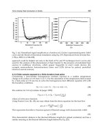
equations but more than two unknown variables in both of the equations. Figure 1 shows
the illustrated scenario with three WMRs in the MRFS.

Fig. 1. A MRFS with three WMRs.

In Figure 1, the interconnected structures:
1
s
F and

2
s
F , are both the solutions. If the
additional nonholonomic constraints in each of the WMRs are called the nonholonomy, the
design challenge of the MRFCS immediately arises that there may be infinite solutions or
conversely no solutions. Thus we can conclude that the conditions of the solution depends
on the nonholonomy. We can further explain that the nonholonomic constraint always
forbids locally to reach some of the neighborhood of the WMR so that the nonholonomic
system with redundent nonholonomy or holonomy equations(ususally the total equation
number is over or equal to the dimension of the system) may not have physical solution.
Now we set oriented direction of the MRFS from
c
q to
1
q tangent to the desired path


c t ,
see Figure 1. With respect to the interconnection stability and the subsystem stability,
Definition 2.2 shall be further modified.
Definition 2.4: Let
ij
z
be piecewise continuous in
t
. The equilibrium point
 
0 0
ij
z 

and
 
0 0
i
q 
in formation variable and individual variable respectively for all
,i j
is
 formation system stable: Definition 2.1 holds and if there exist




0 0ij dij z
j
z t z t

 

and
   
0 0i di q
q t q t

 
then


 
0

,
lim
f
ij dij z
t t t
j
z t z t

 

 
 

and
   
0
,
lim
f
i di
t t t
q t q t

 

 
 
, for all
i
;

 asymptotically formation system stable: Definition 2.1 holds and if there exist
   
0 0ij dij z
j
z t z t

 


and




0 0i di q
q t q t

 
then
   
0
,
lim
f
i di q
t t t
q t q t

 


 

 and
   
lim 0
i di
t
q t q t

 
, for all i ;
 formation system unstable: if it is not formation system stable.
No doubt, Definition 2.4 is more rigorous than Definiton 2.2 particularly it can be put on the
condition after releasing the constraints on the formation state. So far, we got two unsolved
problems in the design of the MRFS: first, the the uniqueness of the solution; second, the
subsystem stability with respect to the interconnection stability.
For the first point, coneptually, the key step is how to select the adequate stable
interconnected structure which corresponds to the number of the additional constraints.
CuttingEdgeRobotics2010232

Actually, this idea is simple but it is much complex than we expect in the design process
resulted by the nonholonomic system of the WMR. As we know, the choice of the state of
the MRFS can be either the relative length or the relative angle or even mix both of them and
they are all capable to be the abstractive variables which are abstracted from the states of the
nonholonomic subsystems. There also exists the nonlinear transfomation between the
position and the oriented angle of the WMR so that, in the MRFS, the relative length couples
the relative angle or vice versa. We, therefore, usually select one of them as the abstractive
variables for simplifing the design complexity. With this aspect, if the minimal
interconnected structure of the MRFS is performed, the process is the way regarded as to
release some redundent abstracted equations. In this research, for this issue, we have

proposed the minimal relization with respect to the stable interconnected structure in the
controller design of the MRFS.
The second issue requires more detail study on the nonholonomic system. The
nonholonomic constraints are assumed to be strictly satisfied in this research for applying
the kinematics of the WMR. Hence, the output of the control velocity and the angular
velocity is limited for avoiding to generate the large torque of the WMR. It immediately
implies us that the unreachable region of the nonholonomic system is locally restricted by
the limited torque. In real application of the MRFS, the desired state is usually given in the
abstracted space. When we switch the interconnected topology, following the Remark 2.3,
the nonholonomic subsystem may not be stable if


 
lim 0
ij dij
t
j
z t z t

 

. In this research,
the Lyapunov based approach is proposed for dealing with this design issue.

3. Interconnected Stability and Formation Control Design

Formally, considering the nonholonomic constraints in a differential type WMR, the
kinematics is able to be written by
i i i
q S u



(1)
where
3
T
i pi i
q q q

 
 
 

denote the state of the WMR;
0 0 1
cos sin 0
T
i
i i
S
q q
 
 

 
 
denotes
the distribution;
 
2

T
i i i
u v w  
denotes the control input. The formation state between
two WMRs is distinctly defined as
pj pi
ij
ij
ij
j i
q q
l
z
q q
 

 

 
 

 
 

 
 


(2)
In contrast to the relative formulation with two WMRs, the formation state to the i

th
WMR
with respect to all j
th
connection without regarding with the interconnection structure is
simply defined as the sum of the relative state:
1
1
p pi pn pi
i ij
j
i n i
q q q q
z z
q q q q
   
   
 
   
   
 
   
   


(3)
and if
i j
,
0

ij
z 
. Taking partial derivative to Eq. (3), we have the following equation:

ij
j
i i
i
j
i j
ij
j
l
z z
z
q q

 
 
  
  
 
 
 
 
 
 
 








(4)
For a MRFS, the neighbours of the i
th
WMR is noted as
j
i
q q
which corresponds to the
interconnected structure and can be equivalently interpreted as an adjacency matrix. The
adjacency matrix(Chung 1949) (or so-called interconnection matrix),
G
A
, is represented as a
binary matrix which is one-one maps from the interconnected structure to the elements of
the matrix, i.e.,
j
q
acts on
i
q
if the element in i
th
row and j
th
column of the matrix equals “1”,

 
, 1
G
A i j 
but if i j

,


, 0
G
A i j

. It is the fact that all of the connections of the i
th
WMR to
the neighbour ones are a set:
 


, 1
ij G
a A i j j n

 
where i and
j
denotes the i
th
raw and

j
th
column in the adjacency matrix. Therefore Eq. (4) could be naturally rewritten as
2
2
T T I
ij
p
ij pij pij ij pij
i
T T J
j j
p
ij pij pij ij pij
ij
a
q I q q q
z
q J q q q
l

  

 

  


  


  
 
 

 

(5)
with
3
T
ij pij ij
q q q

 
 
 

;

2ij
I
ij
ij
a I
l
 
;
2ij
J
ij

ij
a J
l
 
;
2
1 0
0 1
I







;
2
0 1
1 0
J








.

Now we summarize the result to the general formation dynamics form Eq. (1) and Eq. (5):
1 1
1 1
2
j
j
i j
n n
n nj
j
i j
z z
z a
q q
n
z z
z a
q q

 
 
 

 
 
 

 




 
 

 
 

 
 
 







(6)
1 1 1
3
n n n
q S u
n
q S u












(7)
There are totally
5n
equations in Eq. (6-7). Obviously, a number of
3n
physical variables
need to be solved so that we can freely choose
2n
equations as a constraints, for example,
minimizing Eq.(7) subject to Eq.(6) or minimizing the position subject to the heading angle
of each WMRs and Eq.(6) and so forth. However, regarding with the interconnected
structure, two problems yield: first, how to determine the minimal stable interconnected
structure; second, how to guarantee the existence of the solution. For the first question, the
following lemma will help us to make such a design:
Lemma 3.1: Considering the MRFS with a selective interconnection structure with totally
p

connections, the stable minimal connection number of
p
is
2 3n

.
The proof follows the rigidity condition of the two dimensional graph, see (Laman 1970).
Now we begin with the second question for the existence of the MRFS. The existence of the

solution is somehow linked to the subsystem stability if the designed nonholonomic control
can derive the WMR to the admissible region within the control time. In other words, the
existence of the solution is in the sense that there locally exist the reachable states of the
TheFormationStabilityofaMulti-RoboticFormationControlSystem 233

Actually, this idea is simple but it is much complex than we expect in the design process
resulted by the nonholonomic system of the WMR. As we know, the choice of the state of
the MRFS can be either the relative length or the relative angle or even mix both of them and
they are all capable to be the abstractive variables which are abstracted from the states of the
nonholonomic subsystems. There also exists the nonlinear transfomation between the
position and the oriented angle of the WMR so that, in the MRFS, the relative length couples
the relative angle or vice versa. We, therefore, usually select one of them as the abstractive
variables for simplifing the design complexity. With this aspect, if the minimal
interconnected structure of the MRFS is performed, the process is the way regarded as to
release some redundent abstracted equations. In this research, for this issue, we have
proposed the minimal relization with respect to the stable interconnected structure in the
controller design of the MRFS.
The second issue requires more detail study on the nonholonomic system. The
nonholonomic constraints are assumed to be strictly satisfied in this research for applying
the kinematics of the WMR. Hence, the output of the control velocity and the angular
velocity is limited for avoiding to generate the large torque of the WMR. It immediately
implies us that the unreachable region of the nonholonomic system is locally restricted by
the limited torque. In real application of the MRFS, the desired state is usually given in the
abstracted space. When we switch the interconnected topology, following the Remark 2.3,
the nonholonomic subsystem may not be stable if




lim 0

ij dij
t
j
z t z t




. In this research,
the Lyapunov based approach is proposed for dealing with this design issue.

3. Interconnected Stability and Formation Control Design

Formally, considering the nonholonomic constraints in a differential type WMR, the
kinematics is able to be written by
i i i
q S u



(1)
where
3
T
i pi i
q q q

 
 
 


denote the state of the WMR;
0 0 1
cos sin 0
T
i
i i
S
q q
 







denotes
the distribution;
 
2
T
i i i
u v w  
denotes the control input. The formation state between
two WMRs is distinctly defined as
pj pi
ij
ij
ij

j i
q q
l
z
q q
 




 



 



 




(2)
In contrast to the relative formulation with two WMRs, the formation state to the i
th
WMR
with respect to all j
th
connection without regarding with the interconnection structure is

simply defined as the sum of the relative state:
1
1
p pi pn pi
i ij
j
i n i
q q q q
z z
q q q q
   

  
 
   

  
 

  

  


(3)
and if
i j
,
0
ij

z 
. Taking partial derivative to Eq. (3), we have the following equation:

ij
j
i i
i
j
i j
ij
j
l
z z
z
q q

 
 
  
  
 
 
 
 
 
 
 








(4)
For a MRFS, the neighbours of the i
th
WMR is noted as
j
i
q q
which corresponds to the
interconnected structure and can be equivalently interpreted as an adjacency matrix. The
adjacency matrix(Chung 1949) (or so-called interconnection matrix),
G
A
, is represented as a
binary matrix which is one-one maps from the interconnected structure to the elements of
the matrix, i.e.,
j
q
acts on
i
q
if the element in i
th
row and j
th
column of the matrix equals “1”,
 

, 1
G
A i j 
but if i j

,


, 0
G
A i j 
. It is the fact that all of the connections of the i
th
WMR to
the neighbour ones are a set:
 


, 1
ij G
a A i j j n  
where i and
j
denotes the i
th
raw and
j
th
column in the adjacency matrix. Therefore Eq. (4) could be naturally rewritten as
2

2
T T I
ij
p
ij pij pij ij pij
i
T T J
j j
p
ij pij pij ij pij
ij
a
q I q q q
z
q J q q q
l
   

 
   

   
   
 
 

 

(5)
with

3
T
ij pij ij
q q q

 
 
 

;

2ij
I
ij
ij
a I
l
 
;
2ij
J
ij
ij
a J
l
 
;
2
1 0
0 1

I
 

 
 
;
2
0 1
1 0
J

 

 
 
.
Now we summarize the result to the general formation dynamics form Eq. (1) and Eq. (5):
1 1
1 1
2
j
j
i j
n n
n nj
j
i j
z z
z a
q q

n
z z
z a
q q

 
 
 

 
 
 

 



 
 

 
 

 
 
 








(6)
1 1 1
3
n n n
q S u
n
q S u











(7)
There are totally
5n
equations in Eq. (6-7). Obviously, a number of
3n
physical variables
need to be solved so that we can freely choose
2n
equations as a constraints, for example,

minimizing Eq.(7) subject to Eq.(6) or minimizing the position subject to the heading angle
of each WMRs and Eq.(6) and so forth. However, regarding with the interconnected
structure, two problems yield: first, how to determine the minimal stable interconnected
structure; second, how to guarantee the existence of the solution. For the first question, the
following lemma will help us to make such a design:
Lemma 3.1: Considering the MRFS with a selective interconnection structure with totally
p

connections, the stable minimal connection number of
p
is
2 3n 
.
The proof follows the rigidity condition of the two dimensional graph, see (Laman 1970).
Now we begin with the second question for the existence of the MRFS. The existence of the
solution is somehow linked to the subsystem stability if the designed nonholonomic control
can derive the WMR to the admissible region within the control time. In other words, the
existence of the solution is in the sense that there locally exist the reachable states of the
CuttingEdgeRobotics2010234

nonholonomic subsystem such that the WMR moves within the reachable region such that
the sufficient condition of the subsystem stability is achieved.
Moreover, the coupling effect of the states in the WMR has to be considered. The state
equation in Eq. (1) can be generally rewritten as


p
i pi i i
i i
q f q v

q w







(8)
where
2
:
pi
f  
denotes a continuous and differentiable function;
i
v and
i
w denote the
velocity and angular velocity respectively. Eq. (8) clearly represents the coupled effect
between
pi
q
and
i
q

in the nonholonomic system. It may be safety to assume that the
velocity is a constant in the practical control design, the position and oriented angle can be
derived by the assigned angular velocity simultaneously due to non-invloutive

characteristic from Frobenious Thorem(Abraham and Marsden 1967). Conversely, if we set
the angular velocity as a constant, the WMR is restricted to move along a line for the
constrained oriented angle in the abstracted space. (BLOC and CROUC 1998) has indicated
the general design rule of the nonholonomic control design which is stated in the following
Remark:
Remark 3.2: Consider the nonholonomic system in Eq. (8). The system stability holds if the
controller is designed for the WMR whose convergence rate of
i
q

is always faster than the
one of
pi
q
.
Remark 3.2, for the MRFS, implies us that the subsystem stability is able to be designed by
choosing the interconnected structure with respect to the relative length which is the
function of
p
i
q . Through the way, another variable
i
q

is set free and is configurable.
Therefore, the MRFS will be stable if the controller of the MRFS is carefully designed for
satisfying Remark 3.2. Hence the formation dynamics for the i
th
WMR in Eq.(5) could be
further reduced:

 
2
1
T T I
i ij pij pij pij ij pij
j j
ij
z a q I q q q
l
  
 
 


(9)
Rearranging the equation, the canonical form of the MRFS is further obtained with Eq. (6):
 
 


1 1
T I
i pij ij pj j j pi i i
j
n n
z q f q v f q v
q w
q w
 




  
















(10)
Corollary 3.3: Consider the formation dynamics in Eq. (10), the state flow of the MRFS is
equivalent to the state flow of the nonholonomic WMR. It can generally be written as the
following formula:

   
1 2
1 1
, , , , , , , ,
i i ij ij pi pj j i ij ij pi pj i i

j j
n n
z f a z q q q f a z q q q v
q w
q w
 


 
 
 
 


 





(11)
Figure 2. shows the nonholonomic hierarchical structure in the nonholonomic formation
dynamics in Eq. (11).

Fig. 2. the system structure of the nonholonomic formation dynamics.

Remark 3.4: Considering the MRFS, the interconnection matrix can be regarded as a linear
operator of the formation dynamics.
For the Remark 3.4, an immediately result can be observed in Eq. (10). Hence, once the

interconnected structure of the MRFS changes on-line so as to the interconnection matrix,
the formation shape is able to be dynamically modified by applying the operator with the
refreshed interconnection matrix. It is helpful in the implementation of the MRFS.
Now we shall prove the following statement: the interconnection stable is hold if and only if
all of the eigenvalues of the interconnection matrix is positive. Purposely, the Lyapunov
approach is adopted for minimizing the energy generated from the individual WMRs and
the formation system. We select the Lyapunov function:
1
2
T
i ii i i
L
a q q
, in each of the
subsystem. This leads into the convergence rate of the heading angle of the WMR could be
under our control. For helping the judgement, we also define the interconnection Lyapunov
function:
:
1
2
T
ij ij ij ij
j j i
L
a z z



. Following these definitions, the formation Lyapunov function
F

i
L
can be simply split into two parts: the individual Lyapunov function of the i
th
WMR and
the interconnection Lyapunov functions of the j
th
WMR which acts on the i
th
WMR:

F
i i ij
j
L L L 


(12)
TheFormationStabilityofaMulti-RoboticFormationControlSystem 235

nonholonomic subsystem such that the WMR moves within the reachable region such that
the sufficient condition of the subsystem stability is achieved.
Moreover, the coupling effect of the states in the WMR has to be considered. The state
equation in Eq. (1) can be generally rewritten as


p
i pi i i
i i
q f q v

is produced by the
interconnection of the MRFS for the i
th
subsystem. In the component form, it is able to be
written as
1 1
1 1
2 2
T
pi
F T T
i pi i i Gi n n
i
q
L
q q P A z z z z
q


 
 
 
 
 
 
 
 


(13)

where
3 3
i
P

 denotes the positive diagonal matrix of the i
th
WMR;
Gi
A
denotes the i
th
raw
of the interconnection matrix. Hence the necessary condition for the asymptotically
formation stable is established via the following theorem:
Theorem 3.5: Considering the MRFS described in Eq. (11), the system, follows Definition 2.2,
is said to be asymptotically interconnection stable.

Proof. Using Eq. (9), the time derivative of the Eq. (12) can be written as:
 
1 1
2 2
T I T I T I I
ij pij ij pij pij ij pij pij i ij ij i pij
j j j
L
q q q q q F F q
   
       
   

   
  

 

(14)
where
i pi i
F f q  
denotes a linearized matrix from the nonlinear function
pi
f
in Eq. (8). In
order to state the stability condition on the MRFS, the Lyapunov function can be reproduced
by Eq. (14) from single WMR to all WMRs in a formation team. Thus we reformulate the
result in Eq. (14) in associated with a matrix formula:
I I
F F Q    
(15)
where
i
Q
are positive matrix. According to the Lyapunov stability theorem, if
I

and
i
Q

are positive definite, then the MRFS in Eq. (11) is asymptotically stable. Q. E. D.

So far, the analysis result of the interconnection stability reveals us that the sufficient
condition of the formation stable satisfies not only the existence of the positive definite
interconnection matrix but also the subsystem stable by the Definition 2.4. Namely, if the
formation stable holds, the necessary condition is that the interconnection matrix has to be
positive definite. Note that the formation dynamics can be identified without driving the
formation dynamics via Theorem 3.5. Practically, let us now consider the design of the
control of the MRFS. The Lyapunov function in Eq. (12) can be further taken the partial
derivative:
   
1 2
, , , , , , , ,
ij
F
i
i
j
i j
i ij ij pi pj j pi i i ij ij pi pj i i i i
j j
L
L
L
q q
f
a z q q q q S f a z q q q v q w
  


 
 

 
   
 
 

 


(16)
Therefore, the formation control can be chosen by the following Theorem:
Theorem 3.6: Considering the MRFS follows Eq. (11), if the velocity and angular velocity is
chosen by:



 
 
1
2
2
, , , ,
;
, , , ,
0 if , , , , 0;
.
F
i ij ij pi pj j pi i
j
pi i i ij ij pi pj i
i

j
pi i i ij ij pi pj i
j
i i i
f a z q q q K L
q S f a z q q q
v
q S f a z q q q
w K q



 




 


 


 

 

 
 


 

 




(17)
then the MRFS is exponentially stable where
0
pi i
K K

 
denote the constant real number.
Proof: After taking the controller in Eq. (17) into Eq. (16), the Lyapunov equation is
obtained:


2
F
F F
i pi i pi i i pi i
L
K L K K q K L
 
     


(18)

Consequently, the system is exponentially stable.
Remark 3.7 According to Theorem 3.6, the controller is capable of switching the
interconnection structure in real-time by modifying the parameter:
ij
a .
Finally, the proposed formation stability theories and control design process in this section
can be regarded as a useful tool.

4. Simulation

In this section, a simulation is performed for demonstrating the performance of the
proposed nonholonomic multi-robotic formation control with respect to the formation
stability. Figure 3 shows the simulation scenario with four WMRs in the MRFS. The team
begins with the triangular shape and moves along a curve to the target with a square shape
that shall change the interconnected structure on the middle way of the motion curve drawn
as the solid line in Figure 3. Observing the interconnected structures, they satisfy the rigid
condition which implies the interconnection stable of the MRFS in Lemma 3.1 so that the
interconnection stability is promised by Definition 2.2.
TheFormationStabilityofaMulti-RoboticFormationControlSystem 237

In Eq. (12),
i
L
is generated from the i
th
subsystem and
ij
j
L


is produced by the
interconnection of the MRFS for the i
th
subsystem. In the component form, it is able to be
written as
1 1
1 1
2 2
T
pi
F T T
i pi i i Gi n n
i
q
L
q q P A z z z z
q


 


 
 
 
 


 


(13)
where
3 3
i
P

 denotes the positive diagonal matrix of the i
th
WMR;
Gi
A
denotes the i
th
raw
of the interconnection matrix. Hence the necessary condition for the asymptotically
formation stable is established via the following theorem:
Theorem 3.5: Considering the MRFS described in Eq. (11), the system, follows Definition 2.2,
is said to be asymptotically interconnection stable.

Proof. Using Eq. (9), the time derivative of the Eq. (12) can be written as:
 
1 1
2 2
T I T I T I I
ij pij ij pij pij ij pij pij i ij ij i pij
j j j
L
q q q q q F F q
   

       
   
   
  

 

(14)
where
i pi i
F f q  
denotes a linearized matrix from the nonlinear function
pi
f
in Eq. (8). In
order to state the stability condition on the MRFS, the Lyapunov function can be reproduced
by Eq. (14) from single WMR to all WMRs in a formation team. Thus we reformulate the
result in Eq. (14) in associated with a matrix formula:
I I
F F Q

   
(15)
where
i
Q
are positive matrix. According to the Lyapunov stability theorem, if
I

and

i
Q

are positive definite, then the MRFS in Eq. (11) is asymptotically stable. Q. E. D.
So far, the analysis result of the interconnection stability reveals us that the sufficient
condition of the formation stable satisfies not only the existence of the positive definite
interconnection matrix but also the subsystem stable by the Definition 2.4. Namely, if the
formation stable holds, the necessary condition is that the interconnection matrix has to be
positive definite. Note that the formation dynamics can be identified without driving the
formation dynamics via Theorem 3.5. Practically, let us now consider the design of the
control of the MRFS. The Lyapunov function in Eq. (12) can be further taken the partial
derivative:
   
1 2
, , , , , , , ,
ij
F
i
i
j
i j
i ij ij pi pj j pi i i ij ij pi pj i i i i
j j
L
L
L
q q
f
a z q q q q S f a z q q q v q w
  



 
 
 
   
 
 

 


(16)
Therefore, the formation control can be chosen by the following Theorem:
Theorem 3.6: Considering the MRFS follows Eq. (11), if the velocity and angular velocity is
chosen by:



 
 
1
2
2
, , , ,
;
, , , ,
0 if , , , , 0;
.
F

i ij ij pi pj j pi i
j
pi i i ij ij pi pj i
i
j
pi i i ij ij pi pj i
j
i i i
f a z q q q K L
q S f a z q q q
v
q S f a z q q q
w K q



 




 


 


 

 


 
 

 

 




(17)
then the MRFS is exponentially stable where
0
pi i
K K

 
denote the constant real number.
Proof: After taking the controller in Eq. (17) into Eq. (16), the Lyapunov equation is
obtained:


2
F
F F
i pi i pi i i pi i
L
K L K K q K L
 

     


(18)
Consequently, the system is exponentially stable.
Remark 3.7 According to Theorem 3.6, the controller is capable of switching the
interconnection structure in real-time by modifying the parameter:
ij
a .
Finally, the proposed formation stability theories and control design process in this section
can be regarded as a useful tool.

4. Simulation

In this section, a simulation is performed for demonstrating the performance of the
proposed nonholonomic multi-robotic formation control with respect to the formation
stability. Figure 3 shows the simulation scenario with four WMRs in the MRFS. The team
begins with the triangular shape and moves along a curve to the target with a square shape
that shall change the interconnected structure on the middle way of the motion curve drawn
as the solid line in Figure 3. Observing the interconnected structures, they satisfy the rigid
condition which implies the interconnection stable of the MRFS in Lemma 3.1 so that the
interconnection stability is promised by Definition 2.2.
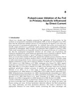
CuttingEdgeRobotics2010238

Fig. 3. the simulation scenario: from triangular to square structure of the MRFS.

In this simulation, we suppose that each of the WMRs is able to know the states from rest of
the WMRs within the control time. Also, the physical configurations for the simulation are
listed: the desired relative length is



12 13 14
5l l l m  
;
 
23 34 24
5 3l l l m   and the initial
relative length is


12 13 14
4l l l m   ;
 
23 34 24
4 3l l l m  
in the triangular shape and


12 24 34 13
5l l l l m    ;
 
14
5 2l m in the squire shape respectively. Considering the
configuration of the single WMR, the initial oriented angles of the WMRs set to zero. The
radius of the active wheels are 0.3( )m and the length of the axis of the active wheels is
0.5( )m . Practically, the control time is set to


0.01 sec

in each of the WMRs.

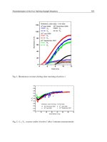
Fig. 4. The trajectory error of the relative length:
23 13 23 14
; ; ;l l l l .

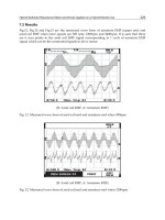
Fig. 5. The error trajectories on the X(red)-Y(blue) Plane from WMR 1-4.

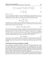
The simulation results are drawn in Figure 4-5 where Figure 4 describes the relative lengths
of the WMRs in the MRFS; Figure 5 draws the tracking error of the WMRs respectively. The
diagrams indicate that the there exists impulse responses on each of the states of the
subsystems when the interconnected structure is changed. In our proposed design, the
subsystem stability can easily be handled.
TheFormationStabilityofaMulti-RoboticFormationControlSystem 239

Fig. 3. the simulation scenario: from triangular to square structure of the MRFS.

In this simulation, we suppose that each of the WMRs is able to know the states from rest of
the WMRs within the control time. Also, the physical configurations for the simulation are
listed: the desired relative length is


12 13 14
5l l l m  
;


23 34 24

5 3l l l m   and the initial
relative length is


12 13 14
4l l l m   ;


23 34 24
4 3l l l m  
in the triangular shape and


12 24 34 13
5l l l l m    ;


14
5 2l m in the squire shape respectively. Considering the
configuration of the single WMR, the initial oriented angles of the WMRs set to zero. The
radius of the active wheels are 0.3( )m and the length of the axis of the active wheels is
0.5( )m . Practically, the control time is set to


0.01 sec
in each of the WMRs.

Fig. 4. The trajectory error of the relative length:
23 13 23 14

; ; ;l l l l .

Fig. 5. The error trajectories on the X(red)-Y(blue) Plane from WMR 1-4.

The simulation results are drawn in Figure 4-5 where Figure 4 describes the relative lengths
of the WMRs in the MRFS; Figure 5 draws the tracking error of the WMRs respectively. The
diagrams indicate that the there exists impulse responses on each of the states of the
subsystems when the interconnected structure is changed. In our proposed design, the
subsystem stability can easily be handled.
CuttingEdgeRobotics2010240

5. Conclusion

The research reveal several important results: first, the formation stability could be
hierarchically decoupled with the interconnection stability and the subsystem stability;
second, the general framework of the MRFS with respect to the nonholonomic subsystems is
obtained; third, the practical exponentially stable formation control is derived with respect
to the minimal interconnection structure of the MRFS that can guarantee the subsystem
stability. Clearly, our study provides a framework for designing and studying the modelling
and the control problem in the nonholonomic MRFS. Finally, the simulation result shows
the control performance so that the approach can be practically used in the switching
interconnected structure of the MRFS on-line without adjusting any control parameters.

6. References

Abraham, R. and J. E. Marsden (1967). Foundations of mechanics. New York, W. A.
Benjamin Inc.
BLOCH, A. M. and P. E. CROUC (1998). "NEWTON'S LAW AND INTEGRABILITY OF
NONHOLONOMIC SYSTEMS." SIAM JOURNAL OF CONTROL
OPTIMIZATION 36(6): 2020-2039.

BLOCH, A. M., S. V. DRAKUNOV, et al. (2000). "STABILIZATION OF NONHOLONOMIC
SYSTEMS USING ISOSPECTRAL FLOWS." SIAM JOURNAL OF CONTROL
OPTIMIZATION 38(3): 855–874.
Brokett, R. W. (1983). "Asymptotic Stability and Feedback Stabilization." Differential
Geometric Control Theory: 181-191.
Chang, C F. and L C. Fu (2008). A Formation Control Framework Based on Lyapunov
Approach. IEEE IROS, Nice, France.
Chung, F. R. K. (1949). Spectral Graph Theory, American Mathematical Society.
Consolinia, L., F. Morbidib, et al. (2008). "Leader–follower formation control of
nonholonomic mobile robots with input constraints." Automatica
.
Das, A. K., R. Fierro, et al. (2002). "A Vision-Based Formation Control Framework." IEEE
TRANSACTIONS ON ROBOTICS AND AUTOMATION 18(5): 813-825.
Desai, J. P., J. P. Ostrowski, et al. (2001). "Modeling and Control of Formation of
Nonholonomic Mobile Robots." IEEE TRANSACTIONS ON ROBOTICS AND
AUTOMATION 17(6).
Fax, J. A. and R. M. Murray (2004). "Information Flow and Cooperative Control of Vehicle
Formations." IEEE TRANSACTIONS ON AUTOMATIC CONTROL
49(9).
Fernandez, O. E. and A. M. Bloch (2008). "Equivalence of The Dynamics of Nonholonomic
And Variational Nonholonomic Systems For Certain Initial Data." Journal of
physics A: Mathematical and Theoretical 41: 1-20.
Harmati, I. and K. Skrzypczyk (2008). "Robot team coordination for target tracking using
fuzzy logic controller in game theoretic framework." Robotics and Automated
System.
Kaminka, G. A., R. Schechter-Glick, et al. (2008). "Using Sensor Morphology for Multirobot
Formations." IEEE TRANSACTIONS ON ROBOTICS AND AUTOMATION
24(2):
271-282.

Keviczky, T., F. Borrelli, et al. (2008). "Decentralized Receding Horizon Control and
Coordination of Autonomous Vehicle Formations." IEEE TRANSACTIONS ON
CONTROL SYSTEMS TECHNOLOGY, 16(1): 19-33.
Koiller, J. (1992). "Reduction of Some Classical Nonholonomic Systems with Symmetry."
Archive for rational mechanics and analysis 118(2): 113-148.
Laman, G. (1970). "On Graphs and Rigidity of Plane Skeletal Structures." Journal of
Engineering Mathematics 4(4): 331-341.
Lin, Z., B. Francis, et al. (2005). "Necessary and Sufficient Graphical Conditions for
Formation Control of Unicycles." IEEE TRANSACTIONS ON AUTOMATIC
CONTROL 50(1): 121-127.
Matinez, S., J. Cortes, et al. (2007). Motion Coordination with Distributed Information. IEEE
Control System Magazine: 75-88.
Monforte, J. C. (2002). Geometric, Control and Numerical Aspects of Nonholonomic
Systems. New Yourk, Springer Verlag.
Murry, R. M. (2007). "Recent Research in Cooperative Control of Multi-Vehicle System."
Journal of Dynamics 129: 571-583.
Murry, R. M. and S. S. Sastry (1993). "Nonholonomic Motion Planning: Steering Using
Sinusoids." IEEE Transaction on Automatic Control 38(5): 700-716.
Olfati-Saber, R. and R. M. Murray (2004). "Consensus Problems in Networks of Agents With
Switching Topology and Time Delay." IEEE TRANSACTIONS ON AUTOMATIC
CONTROL 49(9): 1520-1533.
Pappas, G. J., G. Lafferriere, et al. (2000). "Hierarchically Consistent Control Systems." IEEE
Transactions on Automatic Control 45(6): 1144-1159.
Ren, W. and N. Sorensen (2008). "Distributed coordination architecture for multi-robot
formation control." Robotics and Automated System 56: 324-333.
Singh, M. G. (1977). Dynamical Hierarchical Control. New York, North-Holland.

TheFormationStabilityofaMulti-RoboticFormationControlSystem 241

5. Conclusion

The research reveal several important results: first, the formation stability could be
hierarchically decoupled with the interconnection stability and the subsystem stability;
second, the general framework of the MRFS with respect to the nonholonomic subsystems is
obtained; third, the practical exponentially stable formation control is derived with respect
to the minimal interconnection structure of the MRFS that can guarantee the subsystem
stability. Clearly, our study provides a framework for designing and studying the modelling
and the control problem in the nonholonomic MRFS. Finally, the simulation result shows
the control performance so that the approach can be practically used in the switching
interconnected structure of the MRFS on-line without adjusting any control parameters.

6. References

Abraham, R. and J. E. Marsden (1967). Foundations of mechanics. New York, W. A.
Benjamin Inc.
BLOCH, A. M. and P. E. CROUC (1998). "NEWTON'S LAW AND INTEGRABILITY OF
NONHOLONOMIC SYSTEMS." SIAM JOURNAL OF CONTROL
OPTIMIZATION 36(6): 2020-2039.
BLOCH, A. M., S. V. DRAKUNOV, et al. (2000). "STABILIZATION OF NONHOLONOMIC
SYSTEMS USING ISOSPECTRAL FLOWS." SIAM JOURNAL OF CONTROL
OPTIMIZATION 38(3): 855–874.
Brokett, R. W. (1983). "Asymptotic Stability and Feedback Stabilization." Differential
Geometric Control Theory: 181-191.
Chang, C F. and L C. Fu (2008). A Formation Control Framework Based on Lyapunov
Approach. IEEE IROS, Nice, France.
Chung, F. R. K. (1949). Spectral Graph Theory, American Mathematical Society.
Consolinia, L., F. Morbidib, et al. (2008). "Leader–follower formation control of
nonholonomic mobile robots with input constraints." Automatica.
Das, A. K., R. Fierro, et al. (2002). "A Vision-Based Formation Control Framework." IEEE

TRANSACTIONS ON ROBOTICS AND AUTOMATION 18(5): 813-825.
Desai, J. P., J. P. Ostrowski, et al. (2001). "Modeling and Control of Formation of
Nonholonomic Mobile Robots." IEEE TRANSACTIONS ON ROBOTICS AND
AUTOMATION 17(6).
Fax, J. A. and R. M. Murray (2004). "Information Flow and Cooperative Control of Vehicle
Formations." IEEE TRANSACTIONS ON AUTOMATIC CONTROL 49(9).
Fernandez, O. E. and A. M. Bloch (2008). "Equivalence of The Dynamics of Nonholonomic
And Variational Nonholonomic Systems For Certain Initial Data." Journal of
physics A: Mathematical and Theoretical 41: 1-20.
Harmati, I. and K. Skrzypczyk (2008). "Robot team coordination for target tracking using
fuzzy logic controller in game theoretic framework." Robotics and Automated
System.
Kaminka, G. A., R. Schechter-Glick, et al. (2008). "Using Sensor Morphology for Multirobot
Formations." IEEE TRANSACTIONS ON ROBOTICS AND AUTOMATION 24(2):
271-282.

Keviczky, T., F. Borrelli, et al. (2008). "Decentralized Receding Horizon Control and
Coordination of Autonomous Vehicle Formations." IEEE TRANSACTIONS ON
CONTROL SYSTEMS TECHNOLOGY, 16(1): 19-33.
Koiller, J. (1992). "Reduction of Some Classical Nonholonomic Systems with Symmetry."
Archive for rational mechanics and analysis
118(2): 113-148.
Laman, G. (1970). "On Graphs and Rigidity of Plane Skeletal Structures." Journal of
Engineering Mathematics 4(4): 331-341.
Lin, Z., B. Francis, et al. (2005). "Necessary and Sufficient Graphical Conditions for
Formation Control of Unicycles." IEEE TRANSACTIONS ON AUTOMATIC
CONTROL 50(1): 121-127.
Matinez, S., J. Cortes, et al. (2007). Motion Coordination with Distributed Information. IEEE
Control System Magazine: 75-88.
Monforte, J. C. (2002). Geometric, Control and Numerical Aspects of Nonholonomic

Systems. New Yourk, Springer Verlag.
Murry, R. M. (2007). "Recent Research in Cooperative Control of Multi-Vehicle System."
Journal of Dynamics
129: 571-583.
Murry, R. M. and S. S. Sastry (1993). "Nonholonomic Motion Planning: Steering Using
Sinusoids." IEEE Transaction on Automatic Control 38(5): 700-716.
Olfati-Saber, R. and R. M. Murray (2004). "Consensus Problems in Networks of Agents With
Switching Topology and Time Delay." IEEE TRANSACTIONS ON AUTOMATIC
CONTROL 49(9): 1520-1533.
Pappas, G. J., G. Lafferriere, et al. (2000). "Hierarchically Consistent Control Systems." IEEE
Transactions on Automatic Control 45(6): 1144-1159.
Ren, W. and N. Sorensen (2008). "Distributed coordination architecture for multi-robot
formation control." Robotics and Automated System
56: 324-333.
Singh, M. G. (1977). Dynamical Hierarchical Control
. New York, North-Holland.

CuttingEdgeRobotics2010242
EstimationofUser’sRequestforAttentiveDeskworkSupportSystem 243
EstimationofUser’sRequestforAttentiveDeskworkSupportSystem
YusukeTamura,MasaoSugi,TamioAraiandJunOta
X

Estimation of User's Request for Attentive
Deskwork Support System

Yusuke Tamura, Masao Sugi, Tamio Arai and Jun Ota
The University of Tokyo Japan

1. Introduction

Since the late 1990s, several studies have been conducted on intelligent systems that support
daily life in the home or office environments (Sato et al., 1996; Pentland, 1996; Brooks, 1997). In
daily life, people spend a significant amount of time at desks to operate computers, read and
write documents and books, eat, and assemble objects, among other activities. Therefore it can
be said that supporting deskwork by intelligent systems is of extreme importance. Many kinds
of intelligent systems have been proposed to provide desktop support. In particular,
augmented desk interface systems have been eagerly studied. DigitalDesk is one of the earliest
augmented desk interface systems (Wellner, 1993). It requires a CCD camera and a video
projector to integrate physical paper documents and electronic documents. Koike et al.
proposed EnhancedDesk, which uses an infrared camera instead of a CCD camera to improve
sensitivity to changes in lighting conditions and a complex background (Koike et al., 2001). In
addition, Leibe et al. proposed one called Perceptive Workbench, which requires both a CCD
and an infrared camera (Leibe et al., 2000), and Rekimoto proposed SmartSkin, which is based
on capacitive sensing without cameras (Rekimoto, 2002).
Raghavan et al. proposed a system that requires a head-mounted display to show how to
assemble products (Raghavan et al., 1999). These systems have been limited to show some
information to the user. Ishii & Ullmer proposed an idea referred to as "tangible bits (Ishii &
Ullmer, 1997)," which seeks to realize a seamless interface among humans, digital
information, and the physical environment by using manipulable objects. Based on this idea,
they proposed metaDESK (Ullmer & Ishii, 1997).
Pangaro et al. proposed a system called Actuated Workbench (Pangaro et al., 2002), and
Noma et al. proposed one called Proactive Desk (Noma et al., 2004). Both systems convey
only information to the user through movement of physical objects. They do not support the
user from physical aspects.
On the other hand, especially in rehabilitation robotics, several studies have been conducted
on supporting humans working at desks from a physical aspect (Harwin et al., 1995;
Dallaway et al., 1995). Dallaway & Jackson proposed RAID (Robot for Assisting the
Integration of Disabled people) workstation (Dallaway & Jackson, 1994). In RAID, a user

selects an object through a GUI, and a manipulator carries it to the user. Ishii et al. proposed
a meal-assistance robot for disabled individuals (Ishii et al., 1995). The system user points a
laser attached to his head to operate a manipulator. Topping proposed a system, Handy 1,
16
CuttingEdgeRobotics2010244
which assists severely disabled people with tasks such as eating, drinking, washing, and
shaving (Topping, 2002). In these systems, every time a user wants to be supported, the user
is required to consciously and explicitly instruct their intention to the systems. Such systems
are not really helpful.
Moreover, a few studies have focused on the physical act of passing an object from a human
to a manipulator, or vice versa (Kajikawa et al., 1995; Agah & Tanie, 1997). These studies
focused on the realization of human-like motion of the manipulators. When a user needs to
be supported, on the other hand, the systems are required to support the user as fast as
possible. The studies did not consider the requirement.
In this study, we propose a robotic deskwork support system that delivers objects properly
and quickly to a user who is working at a desk. The intended applications of the proposed
system are assembly, repair, simple experiment, etc. In such applications, the system often
cannot know a sequence of used objects by workers in advance. To achieve the objectives,
the system fulfils two primary functions: It estimates the user
7
s intention, and it delivers
objects to the user.
Intelligent systems are used by ordinary people; therefore, it is important that the systems
be intuitive and simple to use. One of the most intuitive ways to control such systems is
using gestures, especially pointing (Bolt, 1980; Cipolla & Hollinghurst, 1996; Mori et al.,
1998; Sato & Sakane, 2000; Tamura et al., 2004; Sugiyama et al., 2005). Although pointing is
intuitive, it is bothersome for a user to explicitly instruct the systems every time he/she
wants to get objects. Furthermore, as pointing direction can be determined only when the
user's hand and finger remain stationary, the recognition process takes long time. In the
approach proposed here, the system estimates a user's intention inherent in his action

without explicit instructions. In fact, the system 1) detects a user's act of reaching, 2) predicts
the target object required by the user by measuring continuous movement of his body parts,
especially hands and eyes, and finally 3) delivers the object to a user (Figure 1).
predicted target^

Fig. 1. Concept image of the proposed system

In this chapter, the first two items, involving detection and prediction, are mainly described
and discussed.
For the third problem, it is unreasonable to use manipulators for carrying objects. Using
manipulators for delivering objects has the following difficulties:
• Weight capacities of manipulators are generally low for their size.
• As manipulators move three-dimensionally, there is a tremendous danger in
their high-speed movements.
• Because of the large size of manipulators, many manipulators cannot be
operated simultaneously at a desk. Therefore, a manipulator can deliver a
target object only after it grasps the object.
As a result, a system using manipulators cannot quickly and safely support a user.
Moreover, small wheeled mobile robots present problems relative to speed and accuracy of
movement.
One solution for the quick and accurate delivery of multiple objects to a user is to use
movable trays driven with a Sawyer-type 2-DOF stepping motor (Sawyer, 1969). The motors
are small and have high speed, positioning accuracy, and thrust.
The movable tray has high weight capacity, and moves only on a desk plane. Furthermore,
because multiple trays can be placed simultaneously on a desk, multiple objects can be
loaded on the trays. Therefore, a system using the movable trays can quickly and safely
support a user.
In this chapter, we assume that our deskwork support system uses such movable trays and
objects are loaded onto the trays. Assumed size of each tray is 130 x 135 x 25 (mm). In this
study, we assume a normal size desk for the system. The width of a normal desk is at most

1200 (mm). According to this, the number of trays lined up in one row sideways is less than
nine. In order to quickly deliver objects, a straight route is preferable for each tray. Even if
the arrangement of the trays is schemed, the possible number of trays on a desk will be at
most ten. We also assume that the distance between the trays and a user is greater than the
user's reach. This assumption is for not obstructing a user's work.
In order to quickly deliver objects to a user, the trays are required not only to move fast but
also to start early. Considering the speed of the user's hand and the movable trays, the
preparation time for carrying objects (detection of the user's reach and prediction of the
target object) should be less than a half of an average duration of reaching movements.
According to a preliminary experiment, the average duration is about 0.8 (s) without any
help. Therefore, the preparation time should be less than 0.4 (s).
In section 2, an algorithm used to detect reaching movement of a user is presented. A
method used to predict a target object among multiple objects is described in section 3. In
section 4, experiments for verifying the proposed method are described and discussed. In
the experiments, the movable trays are not used. Experiments using the movable trays are
presented in section 5. We conclude this chapter and refer to the future research in section 6.

2. Detection of human reaching movements
To deliver an object to a user, it is necessary that the system determine whether the user is
performing an unrelated task or reaching for the object in question. When an individual
reaches for an object, his hand and eyes move almost simultaneously toward the object. It
has been reported that saccadic eye movement occurs before the onset of a reaching
movement (Prablanc et al., 1979; Biguer et al., 1982; Abrams et al., 1990) and the saccade is
followed about 100 (ms) later by a hand movement (Prablanc et al., 1979). In this study,
therefore, a user's hand movements are measured to detect his reaching movements. When
individuals perform tasks at desks, their hand movements are limited to a specific area, and
their hands turn around frequently. When reaching for objects, on the other hand,
individuals move their hands toward the outside of the working area at a high speed. The
trajectories of hand movements are known to be relatively straight and smooth (Morasso,
1981). In addition to these characteristics of hand movements, eyes move toward a target

EstimationofUser’sRequestforAttentiveDeskworkSupportSystem 245
which assists severely disabled people with tasks such as eating, drinking, washing, and
shaving (Topping, 2002). In these systems, every time a user wants to be supported, the user
is required to consciously and explicitly instruct their intention to the systems. Such systems
are not really helpful.
Moreover, a few studies have focused on the physical act of passing an object from a human
to a manipulator, or vice versa (Kajikawa et al., 1995; Agah & Tanie, 1997). These studies
focused on the realization of human-like motion of the manipulators. When a user needs to
be supported, on the other hand, the systems are required to support the user as fast as
possible. The studies did not consider the requirement.
In this study, we propose a robotic deskwork support system that delivers objects properly
and quickly to a user who is working at a desk. The intended applications of the proposed
system are assembly, repair, simple experiment, etc. In such applications, the system often
cannot know a sequence of used objects by workers in advance. To achieve the objectives,
the system fulfils two primary functions: It estimates the user
7
s intention, and it delivers
objects to the user.
Intelligent systems are used by ordinary people; therefore, it is important that the systems
be intuitive and simple to use. One of the most intuitive ways to control such systems is
using gestures, especially pointing (Bolt, 1980; Cipolla & Hollinghurst, 1996; Mori et al.,
1998; Sato & Sakane, 2000; Tamura et al., 2004; Sugiyama et al., 2005). Although pointing is
intuitive, it is bothersome for a user to explicitly instruct the systems every time he/she
wants to get objects. Furthermore, as pointing direction can be determined only when the
user's hand and finger remain stationary, the recognition process takes long time. In the
approach proposed here, the system estimates a user's intention inherent in his action
without explicit instructions. In fact, the system 1) detects a user's act of reaching, 2) predicts
the target object required by the user by measuring continuous movement of his body parts,
especially hands and eyes, and finally 3) delivers the object to a user (Figure 1).
predicted target^

Fig. 1. Concept image of the proposed system

In this chapter, the first two items, involving detection and prediction, are mainly described
and discussed.
For the third problem, it is unreasonable to use manipulators for carrying objects. Using
manipulators for delivering objects has the following difficulties:
• Weight capacities of manipulators are generally low for their size.
• As manipulators move three-dimensionally, there is a tremendous danger in
their high-speed movements.
• Because of the large size of manipulators, many manipulators cannot be
operated simultaneously at a desk. Therefore, a manipulator can deliver a
target object only after it grasps the object.
As a result, a system using manipulators cannot quickly and safely support a user.
Moreover, small wheeled mobile robots present problems relative to speed and accuracy of
movement.
One solution for the quick and accurate delivery of multiple objects to a user is to use
movable trays driven with a Sawyer-type 2-DOF stepping motor (Sawyer, 1969). The motors
are small and have high speed, positioning accuracy, and thrust.
The movable tray has high weight capacity, and moves only on a desk plane. Furthermore,
because multiple trays can be placed simultaneously on a desk, multiple objects can be
loaded on the trays. Therefore, a system using the movable trays can quickly and safely
support a user.
In this chapter, we assume that our deskwork support system uses such movable trays and
objects are loaded onto the trays. Assumed size of each tray is 130 x 135 x 25 (mm). In this
study, we assume a normal size desk for the system. The width of a normal desk is at most
1200 (mm). According to this, the number of trays lined up in one row sideways is less than
nine. In order to quickly deliver objects, a straight route is preferable for each tray. Even if
the arrangement of the trays is schemed, the possible number of trays on a desk will be at
most ten. We also assume that the distance between the trays and a user is greater than the

user's reach. This assumption is for not obstructing a user's work.
In order to quickly deliver objects to a user, the trays are required not only to move fast but
also to start early. Considering the speed of the user's hand and the movable trays, the
preparation time for carrying objects (detection of the user's reach and prediction of the
target object) should be less than a half of an average duration of reaching movements.
According to a preliminary experiment, the average duration is about 0.8 (s) without any
help. Therefore, the preparation time should be less than 0.4 (s).
In section 2, an algorithm used to detect reaching movement of a user is presented. A
method used to predict a target object among multiple objects is described in section 3. In
section 4, experiments for verifying the proposed method are described and discussed. In
the experiments, the movable trays are not used. Experiments using the movable trays are
presented in section 5. We conclude this chapter and refer to the future research in section 6.

2. Detection of human reaching movements
To deliver an object to a user, it is necessary that the system determine whether the user is
performing an unrelated task or reaching for the object in question. When an individual
reaches for an object, his hand and eyes move almost simultaneously toward the object. It
has been reported that saccadic eye movement occurs before the onset of a reaching
movement (Prablanc et al., 1979; Biguer et al., 1982; Abrams et al., 1990) and the saccade is
followed about 100 (ms) later by a hand movement (Prablanc et al., 1979). In this study,
therefore, a user's hand movements are measured to detect his reaching movements. When
individuals perform tasks at desks, their hand movements are limited to a specific area, and
their hands turn around frequently. When reaching for objects, on the other hand,
individuals move their hands toward the outside of the working area at a high speed. The
trajectories of hand movements are known to be relatively straight and smooth (Morasso,
1981). In addition to these characteristics of hand movements, eyes move toward a target
CuttingEdgeRobotics2010246
object to localize the position of the object for guiding hand movements (Abrams et al.,
1990). Based on the facts reported above, in this study, the deskwork support system
interprets a hand movement as a reaching movement if the following conditions are

satisfied:
• The speed of a hand movement is rapid,
• The trajectory of a hand movement is relatively smooth and straight, and
• The directions of the gaze and hand (see Figure 2) are close, and the hand
and gaze point are far from the head position.
We define a hand movement as the trajectory of the center of a user's hand. To measure
hand movements, we use a color CCD camera attached to a ceiling. The RGB video data is
first converted to the hue, saturation, and value (HSV) space. These values are then
thresholded to acquire binarized hand images. After that, we apply a morphological erosion
operator to the obtained hand region until it becomes smaller than a predetermined
threshold value, and the center of a user's hand is given as the resulting region's center of
mass. This procedure makes the hand's center insensitive to changes of the shape of the
hand image due to a closing or opening motion of the hand (Oka et al., 2002). A tracking
system that requires no physical contact is used to measure head and eye movements.
The parameters are defined in Figure 2.

Fig. 2. Definition of parameters

Head and eye positions are measured three-dimensionally. However, in what follows, all
positions are projected within a desk plane and are considered to be two-dimensional. Thus,
all vectors are also two-dimensional.
h
s
is a vector from the user's head to user's hand at time
s; g
s
is a vector from the user's head to a gaze point; and a vector from the user's head
to object k is denoted by Os. In this study, v
s
, the speed of a hand movement, is defined using

the following equation:

1s s
s
h h
v
t




(1)
where At is the sampling time of the camera.
To enable the system to determine whether a hand movement is a reach or some unrelated
movement is difficult. Failures to detect the target movement can be eliminated by
integrating multiple criteria. Therefore, probabilities are established for three criteria, speed
of hand movement, curvature of hand trajectory, and the relationship between the hand
position and gaze point, which are used to detect the act of reaching.

2.1 Speed of a hand movement
The speed of a hand movement during reaching is much greater than that when performing
tasks that occur close to the trunk of the body.
Therefore, we assume that the faster the relative speed of a user
7
s hand to his head is, the
higher the probability that the hand movement is an act of reaching will be. Here, we adopt
a function whose output ranges between 0 and 1 and increases monotonically with its input
as a probability function. Following this policy, we define
R
v

, the estimated probability from
a hand speed at time s, as the following equation:

 
 
1
,
1 exp
V
s
R
v
 

  
(2)

where
a and ft are parameters representing the motion characteristics of each user.

2.2 Curvature of a hand trajectory
In this study, the curvature of a user's hand trajectory is used as a criterion to indicate
straightness and smoothness.
We regard the curvature of the circle passing through points h
s-2
, h
s-1
, and h
s

as the curvature
of the hand trajectory at time
s (Figure 3).

K
s
is the curvature of the hand trajectory at time s calculated by the following equation:

1 2 1 2
1 2 1 2 2
2
s s s s s
s
s s s s s
h h h h h
K
h h h h h h
   
   
   

  
(3)
As reported earlier, reaching movements are generally straight and smooth. Therefore, the
smaller the curvature of the hand trajectory, the greater the probability that the movement is
Fi
g
. 3. Definition of the curvature of a hand tra
j
ector

y
at time

EstimationofUser’sRequestforAttentiveDeskworkSupportSystem 247
object to localize the position of the object for guiding hand movements (Abrams et al.,
1990). Based on the facts reported above, in this study, the deskwork support system
interprets a hand movement as a reaching movement if the following conditions are
satisfied:
• The speed of a hand movement is rapid,
• The trajectory of a hand movement is relatively smooth and straight, and
• The directions of the gaze and hand (see Figure 2) are close, and the hand
and gaze point are far from the head position.
We define a hand movement as the trajectory of the center of a user's hand. To measure
hand movements, we use a color CCD camera attached to a ceiling. The RGB video data is
first converted to the hue, saturation, and value (HSV) space. These values are then
thresholded to acquire binarized hand images. After that, we apply a morphological erosion
operator to the obtained hand region until it becomes smaller than a predetermined
threshold value, and the center of a user's hand is given as the resulting region's center of
mass. This procedure makes the hand's center insensitive to changes of the shape of the
hand image due to a closing or opening motion of the hand (Oka et al., 2002). A tracking
system that requires no physical contact is used to measure head and eye movements.
The parameters are defined in Figure 2.

Fig. 2. Definition of parameters

Head and eye positions are measured three-dimensionally. However, in what follows, all
positions are projected within a desk plane and are considered to be two-dimensional. Thus,
all vectors are also two-dimensional.
h

s
is a vector from the user's head to user's hand at time
s; g
s
is a vector from the user's head to a gaze point; and a vector from the user's head
to object k is denoted by Os. In this study, v
s
, the speed of a hand movement, is defined using
the following equation:

1s s
s
h h
v
t




(1)
where At is the sampling time of the camera.
To enable the system to determine whether a hand movement is a reach or some unrelated
movement is difficult. Failures to detect the target movement can be eliminated by
integrating multiple criteria. Therefore, probabilities are established for three criteria, speed
of hand movement, curvature of hand trajectory, and the relationship between the hand
position and gaze point, which are used to detect the act of reaching.

2.1 Speed of a hand movement
The speed of a hand movement during reaching is much greater than that when performing
tasks that occur close to the trunk of the body.

Therefore, we assume that the faster the relative speed of a user
7
s hand to his head is, the
higher the probability that the hand movement is an act of reaching will be. Here, we adopt
a function whose output ranges between 0 and 1 and increases monotonically with its input
as a probability function. Following this policy, we define
R
v
, the estimated probability from
a hand speed at time s, as the following equation:

 
 
1
,
1 exp
V
s
R
v
 

  
(2)

where
a and ft are parameters representing the motion characteristics of each user.

2.2 Curvature of a hand trajectory

In this study, the curvature of a user's hand trajectory is used as a criterion to indicate
straightness and smoothness.
We regard the curvature of the circle passing through points h
s-2
, h
s-1
, and h
s
as the curvature
of the hand trajectory at time
s (Figure 3).

K
s
is the curvature of the hand trajectory at time s calculated by the following equation:

1 2 1 2
1 2 1 2 2
2
s s s s s
s
s s s s s
h h h h h
K
h h h h h h
   
   
   

  

(3)
As reported earlier, reaching movements are generally straight and smooth. Therefore, the
smaller the curvature of the hand trajectory, the greater the probability that the movement is
Fi
g
. 3. Definition of the curvature of a hand tra
j
ector
y
at time

CuttingEdgeRobotics2010248
an act of reaching. Based on this, we define ^
S
, the estimated probability from a hand
trajectory at time
s, with the following equation:

s
K
s
R


 (4)
where y is a parameter representing the motion characteristics of each user.

2.3 Relationship between the hand position and gaze point

When an individual reaches for an object, he first locates the object and then reaches for it.
To map the location of the target object, a saccadic eye movement occurs about 100 (ms)
before the reaching motion begins (Prablanc et al., 1979), as reported above. Because the
trajectories of reaching movements are relatively straight (Morasso, 1981), the gaze direction
and the direction from head to hand are supposed to be almost equal during the act of
reaching. Furthermore, in the act of reaching, the hand position and gaze point are farther
from an individual's body (Figure 4-a) than during other unrelated tasks (Figure 4-b).

(a) Reaching for a target object
(b) Performing other tasks
Fig. 4. Relationship between hand position and gaze

Based on these facts, we use the inner products of h
s
and g
s
at time s to detect acts of
reaching.

s S S
I h g  (5)
The large values of
I
s
suggest that the directions of the hand and gaze are close and the hand
position and gaze point are far from the person's head. R
i, the estimated probability from the
relationship between the hand position and gaze point at time s, is defined as follows:

 
 
1
,
1 exp
I
S
R
I
 

  
(6)

where ó and Z are parameters representing the motion characteristics of each user.

2.4 Parameter determination
Because individuals differ in the motion characteristics of their hands and eyes, the five
parameters reported above


, , , , and

   
are required to determine a specific
individual's characteristics.
In this study, we determine the parameters through the following sequence. In this chapter,
we take two parameters of R
v




and


as an example.
1.
A hand movement while a user is performing some tasks and occasionally
reaches for objects is measured.
2.
Acquired velocity data v
s
are discretized into several ranges, and times that a
hand movement in a certain range of velocity is a reaching movement and
those that the movement is not a reaching movement are counted
respectively.
3.



1i i
B s B
p reaching v v v

  , the likelihood that a hand movement in a certain
range of velocity is a reaching movement, is plotted as Figure 5, where
v
B
, is

the boundary value between range
i-1 and range i. Here, because we assume
that the system cannot determine a prior probability p(reaching), we
normalize the observed data.
4.
A curve represented as (2) is fitted to the plotted data points by the
Levenberg-Marquardt method, which is a non-linear least-squares method,
to acquire
a and ¡5 . Here, we adopt the inverse of the probabilities


1i i
B s B
p reaching v v v

  as weight factors for fitting. An example of fitting
R
v
curve
to the observed data points is shown in Figure 5.
The other parameters are determined in the same way.

2.5 Detection of reaching movements
The proposed system detects a hand movement as a reaching movement when R, the
integrated probability at time
s, exceeds the predetermined threshold value. R is defined as
follows:

R = RvRsRi (7)
To reduce missed detections, a large threshold value

To map the location of the target object, a saccadic eye movement occurs about 100 (ms)
before the reaching motion begins (Prablanc et al., 1979), as reported above. Because the
trajectories of reaching movements are relatively straight (Morasso, 1981), the gaze direction
and the direction from head to hand are supposed to be almost equal during the act of
reaching. Furthermore, in the act of reaching, the hand position and gaze point are farther
from an individual's body (Figure 4-a) than during other unrelated tasks (Figure 4-b).

(a) Reaching for a target object
(b) Performing other tasks
Fig. 4. Relationship between hand position and gaze

Based on these facts, we use the inner products of h
s
and g
s
at time s to detect acts of
reaching.

s S S
I h g

 (5)
The large values of
I
s
suggest that the directions of the hand and gaze are close and the hand
position and gaze point are far from the person's head. R
i, the estimated probability from the
relationship between the hand position and gaze point at time s, is defined as follows:




and
 
as an example.
1.
A hand movement while a user is performing some tasks and occasionally
reaches for objects is measured.
2.
Acquired velocity data v
s
are discretized into several ranges, and times that a
hand movement in a certain range of velocity is a reaching movement and
those that the movement is not a reaching movement are counted
respectively.
3.



1i i
B s B
p reaching v v v

  , the likelihood that a hand movement in a certain
range of velocity is a reaching movement, is plotted as Figure 5, where
v
B
, is

r] was used to indicate the distance
between the user's head and hand, which acts as a safety net. Even if
R does not exceed the
predetermined threshold value, the hand movement is detected as an act of reaching when
|| h
s
|| is larger than n . n is a sufficiently large value which is used to prevent missed
detections, and it is empirically set to 400 (mm).
Moreover,
R is set to 0 for a given length of time after detection, where the length of time is
empirically set to 1.0 (s). This rule is used to prevent false detections.
CuttingEdgeRobotics2010250

Hand velocity relative to head (mm/s)
Fig. 5. Fitting a curve of the estimated Rv to the observed probabilities that a hand
movement is a reaching movement

3. Prediction of the target object among multiple objects

People usually use multiple objects at a desk, and the sequence in which the objects are used
is not predetermined. To deliver a required object to a user, a system must be able to
correctly interpret a user's act of reaching at an early stage. It is also necessary that the
system predict the required object as soon as possible.
Accurately predicting the user's hand trajectory seems to offer the right way to predict the
target object. Studies of mathematical models for human arm trajectory planning have
attracted considerable attention; such models include the minimum jerk model (Flash &
Hogan, 1985), the minimum torque change model (Uno et al., 1989), and the minimum
variance model (Harris & Wolpert, 1998). As these models do not consider human trunk
movements and some of them require musculoskeletal parameters that are not easily
acquired, it is difficult to apply them here.

In this study, knowledge of precise trajectories is not necessary; however it is necessary to
identify the target object. There have been several researches on prediction of the target icon
based on movements of a cursor in graphical user interfaces (Balakrishnan, 2004; Asano et
al., 2005), however it cannot be applied to our situation because movements of hands and
cursors are different. The following two assumptions are made to predict the target object.
•
The approach rate of human hand to the target object is higher than to any
other objects in the presence of multiple objects, and
•
When an individual reaches for an object, his gaze directions are distributed
around the direction of the object.
Based on these assumptions, certainty values from hand movements and eye movements
are calculated and integrated probabilistically for each object.

3.1 Inference from hand movements
The certainty that object O
k
is a target object given the trajectory of the user's hand after
starting a reaching movement
H
s
=[ho, h
1
, , h
s
} is defined as follows:

 



 
1
*
k
s
k
S
N
i
s
i
f o
p O O H
f
o

 

(8)

where O* represents the target object and o'
s
is a vector from the user's head to the object O'
('=1, 2, N) at time s. Furthermore, f (o
S
) is calculated with the following equations:
 
   



 
 
 
2
1 1
1
0 0
0
, (9)
0 0
. (10)
k k
s s
k
s
k
s
k k
s
j j j j
k
s
k
j
g o g o
f o
g o
o h o h
g o
o h

 

 

 

 

 
 
  




Equation (10) is transformed into the following equation:

 
0 0
0 0
k k
s s
k
s
k
o h o h
g o
o h
  



(11)

The above equation yields the ratio of the reduction in the distance between the hand and
the object
O
k
from the time the reaching movement is detected (Figure 6).

3.2 Inference from eye movements
In this study, we assume that the user's gaze direction arg(g
s
) follows a wrapped normal
distribution (Gumbel et al., 1953), which is for circular data, with mean arg(o
s
) , the
direction of the target object. Thus, we can represent the conditional probability density
function for arg
(g
s
) = fa
s
given target O
*
=O
k
as the following equation:

 
 

 
 
2
2
arg 2
1
ar
g
* ,
2
2
k
s s
k
s s
o i
p g O O





  


    





 
(12)
where
a is estimated using previous data for each user.

Fi
g
. 6. Prediction of the tar
g
et ob
j
ect on the basis of the ratio of the reduction in the distance
between the hand and the ob
j
ect

EstimationofUser’sRequestforAttentiveDeskworkSupportSystem 251

Hand velocity relative to head (mm/s)
Fig. 5. Fitting a curve of the estimated Rv to the observed probabilities that a hand
movement is a reaching movement

3. Prediction of the target object among multiple objects

People usually use multiple objects at a desk, and the sequence in which the objects are used
is not predetermined. To deliver a required object to a user, a system must be able to
correctly interpret a user's act of reaching at an early stage. It is also necessary that the
system predict the required object as soon as possible.

Accurately predicting the user's hand trajectory seems to offer the right way to predict the
target object. Studies of mathematical models for human arm trajectory planning have
attracted considerable attention; such models include the minimum jerk model (Flash &
Hogan, 1985), the minimum torque change model (Uno et al., 1989), and the minimum
variance model (Harris & Wolpert, 1998). As these models do not consider human trunk
movements and some of them require musculoskeletal parameters that are not easily
acquired, it is difficult to apply them here.
In this study, knowledge of precise trajectories is not necessary; however it is necessary to
identify the target object. There have been several researches on prediction of the target icon
based on movements of a cursor in graphical user interfaces (Balakrishnan, 2004; Asano et
al., 2005), however it cannot be applied to our situation because movements of hands and
cursors are different. The following two assumptions are made to predict the target object.
•
The approach rate of human hand to the target object is higher than to any
other objects in the presence of multiple objects, and
•
When an individual reaches for an object, his gaze directions are distributed
around the direction of the object.
Based on these assumptions, certainty values from hand movements and eye movements
are calculated and integrated probabilistically for each object.

3.1 Inference from hand movements
The certainty that object O
k
is a target object given the trajectory of the user's hand after
starting a reaching movement
H
s
=[ho, h
1

, , h
s
} is defined as follows:

 


 
1
*
k
s
k
S
N
i
s
i
f o
p O O H
f
o

 

(8)

where O* represents the target object and o'
s
is a vector from the user's head to the object O'

('=1, 2, N) at time s. Furthermore, f (o
S
) is calculated with the following equations:
 
   


 
 
 
2
1 1
1
0 0
0
, (9)
0 0
. (10)
k k
s s
k
s
k
s
k k
s
j j j j
k
s
k

j
g o g o
f o
g o
o h o h
g o
o h
 

 

 

 

 
 
  




Equation (10) is transformed into the following equation:

 
0 0
0 0
k k
s s
k

s
k
o h o h
g o
o h
  


(11)

The above equation yields the ratio of the reduction in the distance between the hand and
the object
O
k
from the time the reaching movement is detected (Figure 6).

3.2 Inference from eye movements
In this study, we assume that the user's gaze direction arg(g
s
) follows a wrapped normal
distribution (Gumbel et al., 1953), which is for circular data, with mean arg(o
s
) , the
direction of the target object. Thus, we can represent the conditional probability density
function for arg
(g
s
) = fa
s
given target O

*
=O
k
as the following equation:

 
 
 
 
2
2
arg 2
1
ar
g
* ,
2
2
k
s s
k
s s
o i
p g O O



 
  
 

    
 
 
 
(12)
where
a is estimated using previous data for each user.

Fi
g
. 6. Prediction of the tar
g
et ob
j
ect on the basis of the ratio of the reduction in the distance
between the hand and the ob
j
ect

CuttingEdgeRobotics2010252
3.3 Integration of information from hand and eye movements
The system integrates the probabilities from the user's hand and eye movements based on
Bayes' rule and predicts O, the target object, using the following equation:






 
 
 
*
ˆ
argmax * ,arg
* * arg .
arg max
k
k
s s s
k k
S s s
O
o p O O H g
O O H p O O g
p
   
    
(13)

4. Evaluation of the methods

To examine the usefulness of the methods, experiments were conducted. Generally, human
motion in experiments is not reproducible. If the experiments are conducted in different
conditions, therefore, it is impossible to fairly compare the methods. To tackle this problem,
in this section, we conducted the estimation using three methods for the same human
motion to fairly compare the methods. In the next section, we demonstrated the usefulness
of the proposed method in the system that the movable trays can move.

4.1 Subjects
A total of 11 volunteers (10 males and 1 female, aged 21-42 years old) participated in the
experiments. All subjects were right-handed, and three of them wore eyeglasses.

4.2 Experimental apparatus
An overhead digital color CCD camera (VCC-8350CL, CIS) measured the subjects' hand
movements two-dimensionally.
For image processing, we used a Windows PC (Intel Xeon 3.0GHz Dual) with an image-
processing board (GINGA digital CL-2, Linx) and image-processing software (HALCON7.0,
MVTec).
To measure the subjects' head and eye movements, a head and eye tracking system
(faceLAB4.2, Seeing Machines) that requires no physical contact and a Windows PC (Intel
Pentium4 3.8GHz) were used. The frame rates for the measurement of the hand and eye
movements are 30 (fps) and 60 (fps), respectively. Acquired three-dimensional data were
projected to a desk plane and transformed into two-dimensional data.

4.3 Experimental procedure
In the experiments, subjects assembled a plastic model of a car from five types of
subassemblies (Figure 7) five times, and the movements of each subject's hand, head, and
eyes were recorded.

end product
Fig. 7. Assembly of a plastic model from five types of subassemblies
The subjects reached with their dominant hand (right hand) for the subassemblies. In what
follows, "hand" indicates the dominant hand (right hand). The subjects were asked to grasp
only one type of subassembly at a time.
The arrangement of a subject, a desk, and the subassemblies are shown in Figure 8.
During the experiments, the subjects were asked to sit at the desk and assembled a plastic
model from five types of subassemblies in no particular order.

EstimationofUser’sRequestforAttentiveDeskworkSupportSystem 253
3.3 Integration of information from hand and eye movements
The system integrates the probabilities from the user's hand and eye movements based on
Bayes' rule and predicts O, the target object, using the following equation:





 
 
 
*
ˆ
argmax * ,arg
* * ar
g
.
arg max
k
k
s s s
k k
S s s
O
o p O O H g
O O H p O O g
p
   

    
(13)

4. Evaluation of the methods

To examine the usefulness of the methods, experiments were conducted. Generally, human
motion in experiments is not reproducible. If the experiments are conducted in different
conditions, therefore, it is impossible to fairly compare the methods. To tackle this problem,
in this section, we conducted the estimation using three methods for the same human
motion to fairly compare the methods. In the next section, we demonstrated the usefulness
of the proposed method in the system that the movable trays can move.

4.1 Subjects
A total of 11 volunteers (10 males and 1 female, aged 21-42 years old) participated in the
experiments. All subjects were right-handed, and three of them wore eyeglasses.

4.2 Experimental apparatus
An overhead digital color CCD camera (VCC-8350CL, CIS) measured the subjects' hand
movements two-dimensionally.
For image processing, we used a Windows PC (Intel Xeon 3.0GHz Dual) with an image-
processing board (GINGA digital CL-2, Linx) and image-processing software (HALCON7.0,
MVTec).
To measure the subjects' head and eye movements, a head and eye tracking system
(faceLAB4.2, Seeing Machines) that requires no physical contact and a Windows PC (Intel
Pentium4 3.8GHz) were used. The frame rates for the measurement of the hand and eye
movements are 30 (fps) and 60 (fps), respectively. Acquired three-dimensional data were
projected to a desk plane and transformed into two-dimensional data.

4.3 Experimental procedure
In the experiments, subjects assembled a plastic model of a car from five types of

subassemblies (Figure 7) five times, and the movements of each subject's hand, head, and
eyes were recorded.

end product
Fig. 7. Assembly of a plastic model from five types of subassemblies
The subjects reached with their dominant hand (right hand) for the subassemblies. In what
follows, "hand" indicates the dominant hand (right hand). The subjects were asked to grasp
only one type of subassembly at a time.
The arrangement of a subject, a desk, and the subassemblies are shown in Figure 8.
During the experiments, the subjects were asked to sit at the desk and assembled a plastic
model from five types of subassemblies in no particular order.
CuttingEdgeRobotics2010254
4.4 Experimental results
An example of the observed trajectories of a hand, head, and gaze point is shown in Figure 9.

Fig. 8. Arrangement of an experimental subject, a desk, and five types of subassemblies (O
1
,
O
2
, , O
5
)
. The initial
p
osition of a sub
j
ect's head is around
(

0, -200
)

(
mm
)
.

Fi
g
. 9. Example of the observed tra
j
ectories of hand, head, and
g
aze point while a sub
j
ec
t
reached for 0
2
The observed trajectories of the hand are relatively straight and smooth as presented in the
literature (Morasso, 1981), and the gaze points are distributed around the target object. As
evident in Figure 9, gaze directions are distributed around the target direction. In the
proposed estimation method, detection and prediction processes are independent each
other. Thus we independently examined the usefulness of the detection method and
prediction one.
Detection of reaching movements
We compared the detection performances of the proposed method with those of MD and
MS. MD represents a detection method that uses only a threshold value of distance. MS
represents a detection method uses only a threshold value of hand speed. In MD, we set a

threshold value for the distance between the user's head and hand. When the distance
| | h
s

||
exceeds the predetermined threshold value, the hand movement is detected as a reaching
movement. In MS, we set a threshold value for speed of a hand movement. When the speed
exceeds the predetermined threshold value, the hand movement is detected as a reaching
movement.
We used two metrics, required detection time and detection accuracy, to evaluate the
methods. Because there is a tradeoff between false detections and missed detections, we
defined the detection accuracy using a following equation:

,
correct
correct
f
alse missed
N
DA
N N

 
(14)

where Ncorrect, Nfalse, and Nmissed mean the number of correct detections, false
detections, and missed detections, respectively. The threshold values of MD and MS were
determined for each experimental subject to maximize DA. The required time for detection
and calculated values of DA are shown in Table 1 and Table 2, respectively.
The avera

g
e required time to detect an act of reachin
g
is 0.256 (s). This is about 0.16 (s) shorter
than that of MD and 0.05 (s) longer than that of MS. A total of five acts of reachin
g
went
undetected when the proposed method applied. The reason for the occurrence of the
Table 1. Comparison of the required time (s) to detect an act of reachin
g

EstimationofUser’sRequestforAttentiveDeskworkSupportSystem 255
4.4 Experimental results
An example of the observed trajectories of a hand, head, and gaze point is shown in Figure 9.

Fig. 8. Arrangement of an experimental subject, a desk, and five types of subassemblies (O
1
,
O
2
, , O
5
)
. The initial
p
osition of a sub
j
ect's head is around
(

Cutting Edge Robotics Part 9 docx

Tài liệu liên quan

Tài liệu bạn tìm kiếm đã sẵn sàng tải về