MicroSwimmingRobotsBasedonSmallAquaticCreatures 353

v
x
v
y
t s
v
x
, v
y
mm/s
Hydroglyphus japonicus Sharp

t
= 0.44 ms
L = 2.14 mm
L3
0 0.03 0.06 0.09 0.12
-500
-250
0
250
500

(a) Velocity components of legtip motion


t s
V mm/s
Hydroglyphus japonicus Sharp


t
= 0.44 ms
L = 2.14 mm
L3
0 0.03 0.06 0.09 0.12
250
500

(b) Two dimensional velocity of legtip motion
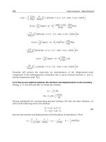
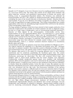
Fig. 11. Velocity variations of legtip motion during swimming of the diving beetle



Fig. 12. Electron micrograph of a part of swimming leg of the diving beetle

resultant velocity is shown in Fig.11(b). Sharp rising up of the velocity variation corresponds
to the power stroke, and gradual decreasing corresponds to the recovery stroke during
swimming of the diving beetle. As stated above, swimming legs of the diving beetle,
Hydroglyphus japonicas Sharp, are also clothed in minute hairs. The hairs increase the
hydrodynamic drag of the swimming leg. Scanning electron microscopic observation of the
swimming legs of the diving beetle shows existence of fine hairs on the legs. Figure 12
shows scanning electron micrograph of the rowing appendages and fine hairs of the diving
beetle, Hydroglyphus japonicas Sharp. The thickness of the hair is about 1.5 μm in Fig.12.

4. Swimming of Dragonfly Nymph

After the dragonfly nymph emerges from the egg, it develops through a series of stages
called instars. The dragonfly larvae are predatory and live in all types of freshwater. The
younger nymph was selected as a test insect in the swimming experiment, because the

younger nymph swam actively. The tested nymph shown in Fig. 13 was a larva of dragonfly,
Sympetrum frequens. The swimming behavior of the nymph in water container was examined.
Fig.14 shows a sequence of photographs showing the swimming behavior of dragonfly



Fig. 13.Photograph of a younger small dragonfly nymph used in the swimming experiment















Fig. 14. A sequence of photographs showing the swimming behavior of the dragonfly
nymph in water container
Biomimetics,LearningfromNature354

nymph. The process of leg movement for the nymph swimming is clear. The fore- and
middle-legs beat almost synchronously. During the power stroke they are stretched and
move. On the other hand, the hind-legs hardly move. The thrust-generating mechanism is
related to the motion of the fore- and middle-legs. The dragonfly nymph expands and

contracts its abdomen to move water during forward swimming. Figure 15 shows the
change in the size of the nymph body through the swimming stroke. The changes of the
body length L
s
and the body width W
s
are the opposite phases. The body length L
s
and the
body width W
s
through the straight swimming are described as follows;






)sin(
)sin(


tWW
tLL
s
s
(8)

where


is the angular frequency of swimming stroke, t is the time,

is the phase difference
with the leg motion, and

and

are constants. In this experiment, constants

and

are
described as follows;






mm25.0
mm60.0


(9)






















Fig. 15. Expansion and contraction of the nymph body during swimming

The change in the body size of tested nymph was about 10%. The legtips move at higher
seed during the power stroke, and lower speed during the recovery stroke. Such a leg

movement generates the thrust force for nymph swimming. The swimming number S
w
of
this tested nymph is the following value;

2.2
1.70.5
6.77




Lf
V
S
s
mean
w
(10)

where V
mean
is the mean swimming velocity, and f
s
is the paddling frequency. The swimming
number shows how many body length per beat to swim. The swimming number S
w
= 2.2 is
larger compared with fish.

5. Micro Swimming Mechanism

5.1 Driving Principle of Micro Swimming Mechanism
The biomimetic study on the swimming robot was performed. As mentioned above, small
aquatic creatures swim by using their swimming legs as underwater paddles to produce
hydrodynamic drag. Based on the above-mentioned swimming analysis of the aquatic
creatures, the micro swimming mechanism was produced by trial and error. The micro
swimming mechanism is composed of polystyrene foam body, permanent magnet,
polyethyleneterephthalate film fin, copper fin stopper, and tin balancer. The dimensions of
the swimming mechanism are shown in Fig.16. The swimming mechanism is propelled by
the magnetic torque acting on the small permanent magnet in the alternating magnetic field.

The magnet is made of NdFeB alloy, and shape is a cube of 5mm×5mm×5mm. Table 1
shows the physical properties of NdFeB permanent magnet used in the experiment. Table 2
shows the magnetic properties of the permanent magnet. The experimental apparatus is
almost similar to Fig.1, but the cylindrical container coiled electric wire was used to drive
the swimming robot. When the alternating magnetic field is applied to the permanent
magnet, the magnet oscillates angularly due to magnetic torque and drives the propulsive
robot in water. The alternating magnetic field was generated by applying AC voltage to the
coil wound around container. The alternating current signal was supplied from a frequency
synthesizer. A block diagram of the coiled water container and measuring devices is shown
in Fig.17. The magnetic torque T
m
acting on the permanent magnet with magnetic moment
m in the external magnetic field H is described by Eq.(11);

HmT
m
 (11)

In this experiment, the external magnetic field was produced by the coil applied AC voltage;

 
tf
E
E
c 0
2sin
2

 (12)


where E is the total amplitude of AC voltage, f
0
is the frequency of AC voltage, and t is the
time. Therefore, the external magnetic field generated by the coil is given by Eq.(13);



tfH
00
2sin

eH  (13)
MicroSwimmingRobotsBasedonSmallAquaticCreatures 355

nymph. The process of leg movement for the nymph swimming is clear. The fore- and
middle-legs beat almost synchronously. During the power stroke they are stretched and
move. On the other hand, the hind-legs hardly move. The thrust-generating mechanism is
related to the motion of the fore- and middle-legs. The dragonfly nymph expands and
contracts its abdomen to move water during forward swimming. Figure 15 shows the
change in the size of the nymph body through the swimming stroke. The changes of the
body length L
s
and the body width W
s
are the opposite phases. The body length L
s
and the
body width W
s
through the straight swimming are described as follows;







)sin(
)sin(


tWW
tLL
s
s
(8)

where

is the angular frequency of swimming stroke, t is the time,

is the phase difference
with the leg motion, and

and

are constants. In this experiment, constants

and

are

described as follows;






mm25.0
mm60.0


(9)






















Fig. 15. Expansion and contraction of the nymph body during swimming

The change in the body size of tested nymph was about 10%. The legtips move at higher
seed during the power stroke, and lower speed during the recovery stroke. Such a leg

movement generates the thrust force for nymph swimming. The swimming number S
w
of
this tested nymph is the following value;

2.2
1.70.5
6.77



Lf
V
S
s
mean
w
(10)

where V
mean
is the mean swimming velocity, and f

s
is the paddling frequency. The swimming
number shows how many body length per beat to swim. The swimming number S
w
= 2.2 is
larger compared with fish.

5. Micro Swimming Mechanism

5.1 Driving Principle of Micro Swimming Mechanism
The biomimetic study on the swimming robot was performed. As mentioned above, small
aquatic creatures swim by using their swimming legs as underwater paddles to produce
hydrodynamic drag. Based on the above-mentioned swimming analysis of the aquatic
creatures, the micro swimming mechanism was produced by trial and error. The micro
swimming mechanism is composed of polystyrene foam body, permanent magnet,
polyethyleneterephthalate film fin, copper fin stopper, and tin balancer. The dimensions of
the swimming mechanism are shown in Fig.16. The swimming mechanism is propelled by
the magnetic torque acting on the small permanent magnet in the alternating magnetic field.
The magnet is made of NdFeB alloy, and shape is a cube of 5mm×5mm×5mm. Table 1
shows the physical properties of NdFeB permanent magnet used in the experiment. Table 2
shows the magnetic properties of the permanent magnet. The experimental apparatus is
almost similar to Fig.1, but the cylindrical container coiled electric wire was used to drive
the swimming robot. When the alternating magnetic field is applied to the permanent
magnet, the magnet oscillates angularly due to magnetic torque and drives the propulsive
robot in water. The alternating magnetic field was generated by applying AC voltage to the
coil wound around container. The alternating current signal was supplied from a frequency
synthesizer. A block diagram of the coiled water container and measuring devices is shown
in Fig.17. The magnetic torque T
m
acting on the permanent magnet with magnetic moment

m in the external magnetic field H is described by Eq.(11);

HmT
m
 (11)

In this experiment, the external magnetic field was produced by the coil applied AC voltage;

 
tf
E
E
c 0
2sin
2

 (12)

where E is the total amplitude of AC voltage, f
0
is the frequency of AC voltage, and t is the
time. Therefore, the external magnetic field generated by the coil is given by Eq.(13);



tfH
00
2sin

eH  (13)

Biomimetics,LearningfromNature356

where H
0
is the amplitude of alternating magnetic field, e is a unit vector. Oscillating torque
motion of the permanent magnet is excited by Eq.(13). The direction of the external magnetic




Fig. 16. Shape and dimension of the micro swimming mechanism

Permanent magnet Nd
2
Fe
14
B
Temperature coefficient 0.12 % / ºC
Density 7300 - 7500 kg/m
3

Curie temperature 310 ºC
Vickers hardness HV 500 - 600
Table 1. Physical properties of permanent magnet used in the experiment

Residual magnetic flux density Br 1.62 - 1.33 T
Coercive force bHC 859 - 970 kA/m
Coercive force iHC > 955 kA/m
Maximum energy product
(BH)

max

302 - 334 kJ/m
3

Table 2. Magnetic properties of NdFeB magnet used in the experiment



Fig. 17. Schematic diagram of experimental apparatus for locomotive characteristics of
swimming robot

field is a vertical direction against the water level as shown in Fig.17. The magnet movement
is connected with the fin motion directly. This mechanism swims by hydrodynamic drag
produced by sweeping the fin. During one cycle of the swimming movement, the fin presses
backwards against the water and this pushes the body forwards.

5.2 Frequency Characteristics of Swimming Velocity
The swimming behavior of the micro mechanism was observed with the experimental
apparatus shown in Fig.17, that is, the swimming velocity of micro mechanism was
examined within a certain frequency range of alternating magnetic field. In this experiment,
the external magnetic field was generated with the coil around the water container shown in
Fig.17. The experiment was performed on the condition of constant E in Eq.(12). Figure 18
shows the frequency characteristics of swimming velocity for the micro mechanism. In
Fig.18, v is the swimming velocity, l is the fin length, w is the fin width, and the dotted lines
show the unstable swimming of the micro mechanism. The effect of the applied voltage E is
also shown in Fig.18. In general, an increase in the applied voltage E improves the
swimming velocity of the micro mechanism. The increase in the applied voltage
corresponds to the increase in the magnetic field generated by the coil. It can be seen from
Fig.18 that the swimming velocity v depends on the frequency of alternating magnetic field

f
0
. The spectrum of the swimming velocity in Fig.18 has the peak at the range of f
0
=4-6Hz.
The peak frequency is related to the oscillation mode of the fin in water. The swimming
velocity of the micro mechanism depends on the amplitude of fin oscillation. The larger
amplitude leads to higher velocity of micro mechanism swimming. The micro mechanism
swims by the fin oscillation. The flow field produced by the fin oscillation was examined.
The flow field around the micro mechanism was visualized by slow shutter speed
photograph. Figure 19 shows one example of flow visualization on the water surface around
the micro mechanism. Flow visualization was created by floating powder on the water
MicroSwimmingRobotsBasedonSmallAquaticCreatures 357

where H
0
is the amplitude of alternating magnetic field, e is a unit vector. Oscillating torque
motion of the permanent magnet is excited by Eq.(13). The direction of the external magnetic



Fig. 16. Shape and dimension of the micro swimming mechanism

Permanent magnet Nd
2
Fe
14
B
Temperature coefficient 0.12 % / ºC
Density 7300 - 7500 kg/m

3

Curie temperature 310 ºC
Vickers hardness HV 500 - 600
Table 1. Physical properties of permanent magnet used in the experiment

Residual magnetic flux density Br 1.62 - 1.33 T
Coercive force bHC 859 - 970 kA/m
Coercive force iHC > 955 kA/m
Maximum energy product
(BH)
max

302 - 334 kJ/m
3

Table 2. Magnetic properties of NdFeB magnet used in the experiment



Fig. 17. Schematic diagram of experimental apparatus for locomotive characteristics of
swimming robot

field is a vertical direction against the water level as shown in Fig.17. The magnet movement
is connected with the fin motion directly. This mechanism swims by hydrodynamic drag
produced by sweeping the fin. During one cycle of the swimming movement, the fin presses
backwards against the water and this pushes the body forwards.

5.2 Frequency Characteristics of Swimming Velocity
The swimming behavior of the micro mechanism was observed with the experimental

apparatus shown in Fig.17, that is, the swimming velocity of micro mechanism was
examined within a certain frequency range of alternating magnetic field. In this experiment,
the external magnetic field was generated with the coil around the water container shown in
Fig.17. The experiment was performed on the condition of constant E in Eq.(12). Figure 18
shows the frequency characteristics of swimming velocity for the micro mechanism. In
Fig.18, v is the swimming velocity, l is the fin length, w is the fin width, and the dotted lines
show the unstable swimming of the micro mechanism. The effect of the applied voltage E is
also shown in Fig.18. In general, an increase in the applied voltage E improves the
swimming velocity of the micro mechanism. The increase in the applied voltage
corresponds to the increase in the magnetic field generated by the coil. It can be seen from
Fig.18 that the swimming velocity v depends on the frequency of alternating magnetic field
f
0
. The spectrum of the swimming velocity in Fig.18 has the peak at the range of f
0
=4-6Hz.
The peak frequency is related to the oscillation mode of the fin in water. The swimming
velocity of the micro mechanism depends on the amplitude of fin oscillation. The larger
amplitude leads to higher velocity of micro mechanism swimming. The micro mechanism
swims by the fin oscillation. The flow field produced by the fin oscillation was examined.
The flow field around the micro mechanism was visualized by slow shutter speed
photograph. Figure 19 shows one example of flow visualization on the water surface around
the micro mechanism. Flow visualization was created by floating powder on the water
Biomimetics,LearningfromNature358

surface. The shutter speed of the camera is 1/2 seconds. The swimming advancement of the
micro mechanism is stopped with the wire of aluminum. The forward and backward flows
are generated, but the backward flow is strongly generated. The speed difference between
forward and backward flows is the swimming speed of the mechanism. Figuer 20 shows the
flowfield produced by the live tethered opposum shrimp for the comparison. A stream is



f
0
Hz
v
m
m
/
s
l =60 mm
w =2 mm
E = 5 V
E = 7 V
E = 10 V
Unstable Behavior
0 10 20 30 40 50 60
10
20
30
40
50
60
70
80

Fig. 18. Frequency characteristics of the micro swimming mechanism





Fig. 19. Flow visualization around the micro swimming mechanism



Fig. 20. Flow visualization around a tethered opossum shrimp in dorsal view

generated by beat motion of swimming legs of the opossum shrimp. The opossum shrimp
swims forward, by pressing the swimming legs backwards against water. The body length
of the opossum shrimp is about 10mm. This photograph was taken with a 35mm camera,
shutter speed at 1/15 s.

6. Diving Beetle Robot

The micro swimming robot was developed experimentally based on the analysis of
swimming behavior of diving beetle. The swimming robot was propelled by the magnetic
torque acting on the small permanent magnet in the external magnetic field. The dimensions
of the diving beetle robot are shown in Fig.21. The swimming robot is composed of vinyl
chloride body, NdFeB permanent magnet, and polyethyleneterephthalate legs. The external
magnetic field was generated by the coil wound round the cylindrical container as shown in
Fig.17. Driving mechanism of the diving beetle robot is shown in Fig.22. Arrows in Fig.22
show direction of the physical quantity or direction of the motion. The magnetic torque T
m
acting on the permanent magnet with magnetic moment m in the external magnetic field H
is given by Eq.(11). The permanent magnet shows the rotational oscillation according to the
direction of the alternating magnetic field as shown in Fig.22. In this experiment, the
external magnetic field was produced by the coil applied AC voltage. The open and shut
motions of the legs occur with the rotational oscillation of the permanent magnet. During
such movements the legs press backwards against the water and this pushes the robot
forwards. Figure 23 shows frequency characteristics of the diving beetle robot swimming.

The swimming velocity of the robot shows the higher value at f
0
=4-12 Hz. The maximum
value of swimming velocity is v
max
=29 mm/s. Then swimming number of the diving robot is
S
w
=0.07. The largest opening angle of the hind leg of real diving beetle is almost θ=π/2.
However, the angle amplitude of robot leg oscillation is ξ =13π /180. Therefore, the
MicroSwimmingRobotsBasedonSmallAquaticCreatures 359

surface. The shutter speed of the camera is 1/2 seconds. The swimming advancement of the
micro mechanism is stopped with the wire of aluminum. The forward and backward flows
are generated, but the backward flow is strongly generated. The speed difference between
forward and backward flows is the swimming speed of the mechanism. Figuer 20 shows the
flowfield produced by the live tethered opposum shrimp for the comparison. A stream is


f
0
Hz
v
m
m
/
s
l =60 mm
w =2 mm E = 5 V
E = 7 V

E = 10 V
Unstable Behavior
0 10 20 30 40 50 60
10
20
30
40
50
60
70
80

Fig. 18. Frequency characteristics of the micro swimming mechanism



Fig. 19. Flow visualization around the micro swimming mechanism



Fig. 20. Flow visualization around a tethered opossum shrimp in dorsal view

generated by beat motion of swimming legs of the opossum shrimp. The opossum shrimp
swims forward, by pressing the swimming legs backwards against water. The body length
of the opossum shrimp is about 10mm. This photograph was taken with a 35mm camera,
shutter speed at 1/15 s.

6. Diving Beetle Robot

The micro swimming robot was developed experimentally based on the analysis of

swimming behavior of diving beetle. The swimming robot was propelled by the magnetic
torque acting on the small permanent magnet in the external magnetic field. The dimensions
of the diving beetle robot are shown in Fig.21. The swimming robot is composed of vinyl
chloride body, NdFeB permanent magnet, and polyethyleneterephthalate legs. The external
magnetic field was generated by the coil wound round the cylindrical container as shown in
Fig.17. Driving mechanism of the diving beetle robot is shown in Fig.22. Arrows in Fig.22
show direction of the physical quantity or direction of the motion. The magnetic torque T
m
acting on the permanent magnet with magnetic moment m in the external magnetic field H
is given by Eq.(11). The permanent magnet shows the rotational oscillation according to the
direction of the alternating magnetic field as shown in Fig.22. In this experiment, the
external magnetic field was produced by the coil applied AC voltage. The open and shut
motions of the legs occur with the rotational oscillation of the permanent magnet. During
such movements the legs press backwards against the water and this pushes the robot
forwards. Figure 23 shows frequency characteristics of the diving beetle robot swimming.
The swimming velocity of the robot shows the higher value at f
0
=4-12 Hz. The maximum
value of swimming velocity is v
max
=29 mm/s. Then swimming number of the diving robot is
S
w
=0.07. The largest opening angle of the hind leg of real diving beetle is almost θ=π/2.
However, the angle amplitude of robot leg oscillation is ξ =13π /180. Therefore, the
Biomimetics,LearningfromNature360

propulsion force produced by leg motion is small. The swimming velocity of the robot was
almost 29 mm/s for f
0

=4-12 Hz, but it depended on the frequency of the alternating
magnetic field.



Fig. 21. Schematic diagram and dimensions of micro diving beetle robot




Fig. 22. Driving mechanism of micro diving beetle robot in swimming propursion



Fig. 23. Frequency characteristics of diving beetle robot in swimming velocity

7. Conclusion

The swimming behavior of small aquatic creatures was analyzed using the high speed video
camera system. Based on the swimming analysis of the aquatic creatures, the micro
swimming mechanism and micro diving robot propelled by alternating magnetic field were
produced. The swimming characteristics of the micro mechanism and micro diving robot
were developed. The swimming mechanism and diving robot swam successfully in the
water. Frequency characteristics of the swimming mechanism and diving beetle robot were
examined. The diving robot showed the higher swimming velocities at f
0
=4-12Hz. These
experiments show the possibility of achievement of the micro robot driving by the wireless
energy supply system. The results obtained are summarized as follows;


(1) In the power stroke of the diving beetle swimming, hind legs are extended and driven
backward to generate forward thrust. While in recovery stroke, hind legs are returned
slowly to their initial position.
(2) In forward swimming of the dragonfly nymph, only the fore pair and the middle pair of
legs are active as a thrust generator. The orbits of fore- and middle-legs show almost the
same, and draw the circle partially of the orbit.
(3) The micro swimming mechanism composed of the NdFeB permanent magnet and film
fin are driven by the alternating magnetic field. The swimming velocity of the micro
mechanism depends on the frequency of alternating magnetic field at the constant voltage.
(4) Flow visualization around the micro mechanism was created by the motion of powder
and slow shutter speed photographic technique. The forward and backward surface flows
and vortex flows around the micro mechanism were generated by the robot driving.
(5) Visualization photographs of flow field around the tethered opossum shrimp show the
generation of tow votices in right and left sides of the body.
(6) The diving robot can dive into the water by sweeping the frequency of magnetic field.
The diving robot can swim backward by the change of magnetic field frequency.

MicroSwimmingRobotsBasedonSmallAquaticCreatures 361

propulsion force produced by leg motion is small. The swimming velocity of the robot was
almost 29 mm/s for f
0
=4-12 Hz, but it depended on the frequency of the alternating
magnetic field.


Fig. 21. Schematic diagram and dimensions of micro diving beetle robot




Fig. 22. Driving mechanism of micro diving beetle robot in swimming propursion



Fig. 23. Frequency characteristics of diving beetle robot in swimming velocity

7. Conclusion

The swimming behavior of small aquatic creatures was analyzed using the high speed video
camera system. Based on the swimming analysis of the aquatic creatures, the micro
swimming mechanism and micro diving robot propelled by alternating magnetic field were
produced. The swimming characteristics of the micro mechanism and micro diving robot
were developed. The swimming mechanism and diving robot swam successfully in the
water. Frequency characteristics of the swimming mechanism and diving beetle robot were
examined. The diving robot showed the higher swimming velocities at f
0
=4-12Hz. These
experiments show the possibility of achievement of the micro robot driving by the wireless
energy supply system. The results obtained are summarized as follows;

(1) In the power stroke of the diving beetle swimming, hind legs are extended and driven
backward to generate forward thrust. While in recovery stroke, hind legs are returned
slowly to their initial position.
(2) In forward swimming of the dragonfly nymph, only the fore pair and the middle pair of
legs are active as a thrust generator. The orbits of fore- and middle-legs show almost the
same, and draw the circle partially of the orbit.
(3) The micro swimming mechanism composed of the NdFeB permanent magnet and film
fin are driven by the alternating magnetic field. The swimming velocity of the micro
mechanism depends on the frequency of alternating magnetic field at the constant voltage.
(4) Flow visualization around the micro mechanism was created by the motion of powder

and slow shutter speed photographic technique. The forward and backward surface flows
and vortex flows around the micro mechanism were generated by the robot driving.
(5) Visualization photographs of flow field around the tethered opossum shrimp show the
generation of tow votices in right and left sides of the body.
(6) The diving robot can dive into the water by sweeping the frequency of magnetic field.
The diving robot can swim backward by the change of magnetic field frequency.

Biomimetics,LearningfromNature362

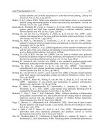
8. References

Alexander, R. McN. (1984). The Gaits of Bipedal and Quadrupedal Animals. The International
Journal of Robotics Research, Vol.3, No.2, pp.49-59
Azuma, A. (1992). The Biokinetics of Flying and Swimming, pp.1-265, Springer-Verlag, ISBN 4-
431-70106-0, Tokyo
Blake, J. (1972). A model for the micro-structure in ciliated organisms. Journal of Fluid
Mechanics, Vol.55, pp.1-23
Dickinson, M.H.; Farley, C.T.; Full, R.J.; Koehl, M.A.R.; Kram, R. & Lehman, S. (2000). How
animals move: An integrative view. Science, Vol.288, No.4, pp.100-106
Dresdner, R.D.; Katz, D.F. & Berger, S.A. (1980). The propulsion by large amplitude waves
of untiflagellar micro-organisms of finite length. Journal of Fluid Mechanics, Vol.97,
pp.591-621
Jiang, H.; Osborn, T.R. & Meneveau, C. (2002a). The flow field around a freely swimming
copepod in steady motion. PartⅠ: Theoretical analysis. Journal of Plankton Research,
Vol.24, No.3, pp.167-189
Jiang, H.; Osborn, T.R. & Meneveau, C. (2002b). The flow field around a freely swimming
copepod in steady motion. PartⅡ: Numerical simulation. Journal of Plankton
Research, Vol.24, No.3, pp.191-213
Jiang, H.; Osborn, T.R. & Meneveau, C. (2002c). Chemoreception and the deformation of the
active space in freely swimming copepods: a numerical study. Journal of Plankton

Research, Vol.24, No.5, pp.495-510
Nachtigall, W. (1980a). Mechanics of swimming in water-beetles, In: Aspects of animal
movement, Elder, H.Y. & Trueman, E.R., pp.107-124, Cambridge University Press,
Cambridge
Nachtigall, W. (1980b). Swimming Mechanics and Energetics of Lovomotion of Variously
Sized Water Beetles- Dytiscidae, Body Length 2 to 35 mm, In: Aspects of animal
movement, Elder, H.Y. & Trueman, E.R., pp.269-283, Cambridge University Press,
Cambridge
Sudo, S.; Tsuyuki, K. & Honda, T. (2008). Swimming mechanics of dragonfly nymph and the
application to robotics. International Journal of Applied Electromagnetics and
Mechanics, Vol.27, pp.163-175
Sudo, S.; Sekine, K.; Shimizu, M.; Shida, S.; Yano, T. & Tanaka, Y. (2009). Basic Study on
Swimming of Small Aquatic Creatures. Journal of Biomechanical Science and
Engineering, Vol.4, No.1, pp.23-36
Zborowski, P. & Storey, R. (1995). A Field Guide to Insects in Australia, pp.111-112, Reed
Books Australia, ISBN 0-7301-0414-1, Victoria

Bio-InspiredWaterStriderRobotswithMicrofabricatedFunctionalSurfaces 363
Bio-Inspired Water Strider Robots with Microfabricated Functional
Surfaces
KenjiSuzuki
X

Bio-Inspired Water Strider Robots with
Microfabricated Functional Surfaces

Kenji Suzuki
Kogakuin University
Japan


1. Introduction

In recent years, there has been considerable interest in insect-inspired miniature robots.
Through evolutionary processes, insects have prospered by adapting themselves to diverse
environments. The number of species of insects is approximately one million, which
comprises approximately two-thirds of all species of animals. By taking advantage of scaling
effects, insects have acquired unique locomotive abilities, such as hexapedal walking,
climbing on walls, jumping, and flying by flapping, that markedly extend their fields of
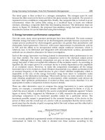
activity. The working principles behind these behaviours are considered to be highly
efficient and optimized for miniature systems. Therefore, they provide alternative design
rules for developing smart and advanced microrobotic mechanisms. For example, the
flapping motion of insect wings has been investigated for micromechanical flying robots
(Suzuki, et al., 1994;
Wood, 2008). This chapter focuses on the locomotion of water striders.
This motion is dependent on surface tension. Recent studies have demonstrated the
mechanisms that enable insects to stay, as well as move, on water. Furthermore, various
kinds of miniature robots that are able to move on water have been developed. Hu et al.
identified the mechanism of the momentum transfer that is responsible for water strider
locomotion and proposed a mechanical water strider driven by elastic thread (Hu, et al.,
2003). Gao et al. showed that the legs of water striders are covered with thousands of tiny
hairs that have fine nanoscale grooves (Gao & Jiang, 2004). These hierarchical micro- and
nanostructures create super-hydrophobic surfaces. Suhr et al. developed a water strider
robot that is driven in one of its resonant modes by using unimorph piezoelectric actuators
(Suhr, et al., 2005). Song et al. numerically calculated the statics of rigid and flexible
supporting legs (Song, et al., 2006; Song, et al., 2007a) and developed a non-tethered water
strider robot using two miniature DC motors and a lithium-polymer battery (Song & Sitti,
2007b). The locomotion mechanisms of fisher spider (Suter & Wildman, 1997; Suter, et al.,
1999) and basilisk lizard (Glasheen & McMahon, 1996a; 1996b) on the surface of water were
studied. A robot that mimics the water running ability of the basilisk lizard was also
developed (Floyd, et al., 2006; Floyd & Sitti, 2008).

The present authors (Suzuki, et al., 2007) have fabricated hydrophobic supporting legs with
microstructured surfaces utilizing MEMS (microelectromechanical systems) techniques, and
18
Biomimetics,LearningfromNature364


(a) Water strider (b) Tip of its leg
Fig. 1.The water strider, used as the robot model

developed non-tethered water strider robots with MEMS-structured legs. In this study,
equations for the forces acting on a partially submerged supporting leg were derived
analytically, and the effects of the diameter and contact angle of the leg on the forces were
investigated. Then, various kinds of hydrophobic supporting legs with and without
microfabricated surfaces were prepared, and the lift and pull-off forces on the water surface
were measured to verify the theoretical analyses. In addition, two non-tethered mechanisms
for water strider robots with microfabricated legs were created to demonstrate autonomous
locomotion on the surface of water.

2. Theoretical model of a supporting leg
2.1 Lift force
Water striders can stay and move on the surface of water by primarily using surface tension
force. Figure 1 shows a water strider on a water surface and an SEM image of the tip of its
leg. The leg is covered with tiny hairs, which improve the hydrophobicity and reduce the
drag force. In this section, equations of the buoyancy and surface tension forces acting on a
partially submerged cylindrical leg are analytically derived
Figure 2 shows a two-dimensional model of the supporting leg. We assume that the leg is a
long, rigid cylinder of uniform material with radius r and contact angle
θ
c
. The vertical lift

force F acting on the leg of unit length consists of a buoyancy force F
B
and a force due to
surface tension F
S
.

B S
F F F
= +

(1)

x
original free surface
water
O
x
0
R
S
2
θ
0
θ
c
γ
S
2
γ

h
p
r
S
1
φ
0
z
0
3-phase
contact line
(x, z)
x = f (z)
γ
γ
F
S
p
F
B
Surface tension
force
Buoyancy
force
θ
0
θ

Fig. 2. Two dimensional model of the supporting leg.


The buoyancy force F
B
is deduced by integrating the vertical component of hydrostatic
pressure p over the body area in contact with the water. The force due to surface tension F
S

is the vertical component of the surface tension per unit length
γ
acting on the three-phase
contact line. Keller demonstrated that F
B
and F
S
are equal to the weights of water displaced
inside and outside of the three-phase contact line, respectively (Keller, 1998). That is, F
B
is
proportional to the area S
1
, shown in Fig. 2, and F
S
is proportional to the area S
2
.

0
0
cos
B
F p r d

φ
φ φ
= ⋅
∫
1
g S
ρ
=

2 2
0 0 0 0 0
( 2 sin sin cos )g z r r r
ρ φ φ φ φ
= − − +

(2)

0 2
2 sin
S
F g S
γ θ ρ
= =

(3)

where
φ
0
is the submerged angle and

θ
0
is the slope of the water surface, as shown in Fig. 2.
The subscript “0” represents the value on the three-phase contact line. The relationship
between
φ
0
and
θ
0
is given by:

0 0 c
φ π θ θ
= + −

(4)

From the Young-Laplace equation, hydrostatic pressure on the surface of water is:

p g z
R
γ
ρ
= − =

(5)

where R is the radius of curvature of the water surface. The governing equation of the
water’s surface profile as a function of z,

( )x f z=
is given by

( )
3
2
2
( )
Sign( )
1 ( )
g z f z
z
f z
ρ
γ
′′
=
′
+

(6)

The boundary conditions for f (z) are

(0)f = ∞
,
0 0 0
( ) sinf z x r
φ
= =


(7)

By integrating (6) by z under the conditions (7), the following equation is obtained:

2
2
( )
1 Sign( ) 1 cos
2
1 ( )
g z f z
z
f z
ρ
θ
γ
′
= + = −
′
+

(8)

Bio-InspiredWaterStriderRobotswithMicrofabricatedFunctionalSurfaces 365


(a) Water strider (b) Tip of its leg
Fig. 1.The water strider, used as the robot model


developed non-tethered water strider robots with MEMS-structured legs. In this study,
equations for the forces acting on a partially submerged supporting leg were derived
analytically, and the effects of the diameter and contact angle of the leg on the forces were
investigated. Then, various kinds of hydrophobic supporting legs with and without
microfabricated surfaces were prepared, and the lift and pull-off forces on the water surface
were measured to verify the theoretical analyses. In addition, two non-tethered mechanisms
for water strider robots with microfabricated legs were created to demonstrate autonomous
locomotion on the surface of water.

2. Theoretical model of a supporting leg
2.1 Lift force
Water striders can stay and move on the surface of water by primarily using surface tension
force. Figure 1 shows a water strider on a water surface and an SEM image of the tip of its
leg. The leg is covered with tiny hairs, which improve the hydrophobicity and reduce the
drag force. In this section, equations of the buoyancy and surface tension forces acting on a
partially submerged cylindrical leg are analytically derived
Figure 2 shows a two-dimensional model of the supporting leg. We assume that the leg is a
long, rigid cylinder of uniform material with radius r and contact angle
θ
c
. The vertical lift
force F acting on the leg of unit length consists of a buoyancy force F
B
and a force due to
surface tension F
S
.

B S
F F F= +


(1)

x
original free surface
water
O
x
0
R
S
2
θ
0
θ
c
γ
S
2
γ
h
p
r
S
1
φ
0
z
0
3-phase

contact line
(x, z)
x = f (z)
γ
γ
F
S
p
F
B
Surface tension
force
Buoyancy
force
θ
0
θ

Fig. 2. Two dimensional model of the supporting leg.

The buoyancy force F
B
is deduced by integrating the vertical component of hydrostatic
pressure p over the body area in contact with the water. The force due to surface tension F
S

is the vertical component of the surface tension per unit length
γ
acting on the three-phase
contact line. Keller demonstrated that F

B
and F
S
are equal to the weights of water displaced
inside and outside of the three-phase contact line, respectively (Keller, 1998). That is, F
B
is
proportional to the area S
1
, shown in Fig. 2, and F
S
is proportional to the area S
2
.

0
0
cos
B
F p r d
φ
φ φ
= ⋅
∫
1
g S
ρ
=

2 2

0 0 0 0 0
( 2 sin sin cos )g z r r r
ρ φ φ φ φ
= − − +

(2)

0 2
2 sin
S
F g S
γ θ ρ
= =

(3)

where
φ
0
is the submerged angle and
θ
0
is the slope of the water surface, as shown in Fig. 2.
The subscript “0” represents the value on the three-phase contact line. The relationship
between
φ
0
and
θ
0

is given by:

0 0 c
φ π θ θ
= + −

(4)

From the Young-Laplace equation, hydrostatic pressure on the surface of water is:

p g z
R
γ
ρ
= − =

(5)

where R is the radius of curvature of the water surface. The governing equation of the
water’s surface profile as a function of z,
( )x f z=
is given by

( )
3
2
2
( )
Sign( )
1 ( )

g z f z
z
f z
ρ
γ
′′
=
′
+

(6)

The boundary conditions for f (z) are

(0)f = ∞
,
0 0 0
( ) sinf z x r
φ
= =

(7)

By integrating (6) by z under the conditions (7), the following equation is obtained:

2
2
( )
1 Sign( ) 1 cos
2

1 ( )
g z f z
z
f z
ρ
θ
γ
′
= + = −
′
+

(8)

Biomimetics,LearningfromNature366

where
θ
is the slope of the water surface (
( ) cotf z
θ
′
=
). Then, the following equations can
be derived from (8).

Sign( ) 2(1 cos )
c
z L
θ θ

= − −

(9)
c
L
g
γ
ρ
=

(10)
2 2
2 2
2
( )
4
c
c
L z
f z
z L z
−
′
=
− −

(11)

where L
c

is the capillary length. By integrating (11) by z, the equation of the surface profile of
the water is given analytically:

1 2 2
2
( ) cosh 4
| |
c
c c
L
x f z L L z C
z
−
 
= = − − +
 
 

(12)

The integration constant C can be determined from the boundary conditions (7). Figure 3
shows the water surface profile given by (12). Since the maximum one-sided width of a
water dimple or bump is approximately 10 mm, the maximum lift force of two supporting
legs whose spacing is less than 20 mm decreases due to two water dimples overlapping
with one another.
From (3), the force due to surface tension F
S
reaches a maximum value 2
γ
at

0
/ 2
θ π
=
if the
surface of the supporting leg is hydrohphobic (
θ
c
>
π
/2). Under this condition, the depth of
the three-phase contact line is
2
c
L
, as shown in Fig.4 (a).

o
max
( ) 2 0.146 N/m (at 20 C)
S
F
γ
= =

(13)

o
0
2 3.86 mm (at 20 C)

c
z L= − = −

(14)


Fig. 3. Profile of the dimple and the bump of water.


(a) Maximum surface tension force (b) Maximum depth of (c) Maximum depth of
of a hydrophobic leg a hydrophobic leg a hydrophilic leg
Fig. 4. Water breaking conditions

Both the maximum surface tension force and the depth of the leg do not depend on the
diameter of the leg or the contact angle. In contrast, the buoyancy force F
B
does depend on
the diameter of the supporting leg. When the diameter is much smaller than L
c
, the force
due to surface tension dominates over the buoyancy force. As the depth of the three-phase
contact line exceeds
2
c
L
,
θ
0
becomes greater than
π

/2 , and the surface tension force
decreases with increasing depth. Figure 4 (b) shows the overhanging water surface just
before the surface is broken.
When the surface of the supporting leg is hydrophlic (
θ
0
<
π
/2), the maximum surface
tension force is 2
γ
sin
θ
c
, which decreases with decreasing the contact angle
θ
c
(Fig. 4 (c)).

2.2 Pull-off force
When the leg is lifted out of the water, water rises with the leg, as shown in Fig. 5 (a). Both
the buoyancy force and the force due to surface tension, given by (2) and (3), respectively,
become negative, that is, downward forces. In this paper, the force needed to lift the leg
from the water is defined as the pull-off force. Figure 5 (b) shows the water surface profile
just before the leg is completely pulled off when the surface of the supporting leg is
hydrophobic. In this situation, the buoyancy force becomes zero, and the maximum pull-off
force is given by (15)
z
θ
c

S
2
< 0
γ
θ
0
< 0
S
1
γ
S
2
< 0
r
φ
0
z
0
p
x
O
R< 0
h

S
2
γ
S
2
γ

θ
c
φ
0
S
1
z
h
x
γ
x
O
S
2
z
θ
c
γ
h

(a) Negative surface tension (b) Maximum pull-off force (c) Maximum pull-off force
and buoyancy forces of a hydropobic leg of a hydrophilic leg
Fig. 5. Pull-off force
Bio-InspiredWaterStriderRobotswithMicrofabricatedFunctionalSurfaces 367

where
θ
is the slope of the water surface (
( ) cotf z
θ

′
=
). Then, the following equations can
be derived from (8).

Sign( ) 2(1 cos )
c
z L
θ θ
= − −

(9)
c
L
g
γ
ρ
=

(10)
2 2
2 2
2
( )
4
c
c
L z
f z
z L z

−
′
=
− −

(11)

where L
c
is the capillary length. By integrating (11) by z, the equation of the surface profile of
the water is given analytically:

1 2 2
2
( ) cosh 4
| |
c
c c
L
x f z L L z C
z
−
 
= = − − +
 
 

(12)

The integration constant C can be determined from the boundary conditions (7). Figure 3

shows the water surface profile given by (12). Since the maximum one-sided width of a
water dimple or bump is approximately 10 mm, the maximum lift force of two supporting
legs whose spacing is less than 20 mm decreases due to two water dimples overlapping
with one another.
From (3), the force due to surface tension F
S
reaches a maximum value 2
γ
at
0
/ 2
θ π
=
if the
surface of the supporting leg is hydrohphobic (
θ
c
>
π
/2). Under this condition, the depth of
the three-phase contact line is
2
c
L
, as shown in Fig.4 (a).

o
max
( ) 2 0.146 N/m (at 20 C)
S

F
γ
= =

(13)

o
0
2 3.86 mm (at 20 C)
c
z L= − = −

(14)


Fig. 3. Profile of the dimple and the bump of water.


(a) Maximum surface tension force (b) Maximum depth of (c) Maximum depth of
of a hydrophobic leg a hydrophobic leg a hydrophilic leg
Fig. 4. Water breaking conditions

Both the maximum surface tension force and the depth of the leg do not depend on the
diameter of the leg or the contact angle. In contrast, the buoyancy force F
B
does depend on
the diameter of the supporting leg. When the diameter is much smaller than L
c
, the force
due to surface tension dominates over the buoyancy force. As the depth of the three-phase

contact line exceeds
2
c
L
,
θ
0
becomes greater than
π
/2 , and the surface tension force
decreases with increasing depth. Figure 4 (b) shows the overhanging water surface just
before the surface is broken.
When the surface of the supporting leg is hydrophlic (
θ
0
<
π
/2), the maximum surface
tension force is 2
γ
sin
θ
c
, which decreases with decreasing the contact angle
θ
c
(Fig. 4 (c)).

2.2 Pull-off force
When the leg is lifted out of the water, water rises with the leg, as shown in Fig. 5 (a). Both

the buoyancy force and the force due to surface tension, given by (2) and (3), respectively,
become negative, that is, downward forces. In this paper, the force needed to lift the leg
from the water is defined as the pull-off force. Figure 5 (b) shows the water surface profile
just before the leg is completely pulled off when the surface of the supporting leg is
hydrophobic. In this situation, the buoyancy force becomes zero, and the maximum pull-off
force is given by (15)
z
θ
c
S
2
< 0
γ
θ
0
< 0
S
1
γ
S
2
< 0
r
φ
0
z
0
p
x
O

R< 0
h

S
2
γ
S
2
γ
θ
c
φ
0
S
1
z
h
x
γ
x
O
S
2
z
θ
c
γ
h

(a) Negative surface tension (b) Maximum pull-off force (c) Maximum pull-off force

and buoyancy forces of a hydropobic leg of a hydrophilic leg
Fig. 5. Pull-off force
Biomimetics,LearningfromNature368

2 cos 0
c
F
γ θ
= <

(15)

Equation (15) indicates that a leg with a large contact angle can easily be lifted from the
water surface. Therefore, super-hydrophobic legs of a water strider reduce the pull-off force
instead of generating a large lift force. When the surface of the supporting leg is hydrophilic,
the maximum pull-off force is approximately 2
γ
if the surface tension effect is dominant,
which does not depend on the contact angle
θ
c
, as shown in Fig. 5 (c).

2.3 Results of the simulations
Using the theoretical model shown in the previous section, the relationship between the
height of the supporting leg, h, and the force acting on the leg, F, was investigated, where h
is defined as the height of the bottom of the supporting leg from the free water surface,
given by:

0 0

(1 cos )h z r
φ
= − −

0 0 0
Sign( ) 2 (1 cos ) (1 cos )
c
L r
θ θ φ
= − − − −

(16)

The force F can be obtained by equations (1) through (4). Thus, h and F are connected by the
parameter
θ
0
.
The results of the calculations are shown in Fig.6. Figure 6 (a) demonstrates the effects of the
contact angle of the leg surface on the lift and pull-off forces. The pull-off force is shown as
the negative lift force. The results show that the lift force of the hydrophobic leg (
θ
c
> 90
o
)
does not differ much due to the contact angle of the leg. In contrast, both the pull-off force
and the height where the leg is completely pulled off increase as the contact angle decreases.
In the case of th hydrophilic leg (
θ

c
< 90
o
), the lift force decreases as the contact angle
decreases and the pull-off force is almost constant. Figure 6 (b) shows the effects of the
diameter of the hydrophobic supporting leg on the lift and pull-off forces. The component of
buoyancy force (F
B
) is also shown in the same figure. The lift force increases as the diameter
of the leg increases. The differences in lift force are derived from the differing buoyancy
forces (F
B
) that depend on the leg diameter. When the diameter of the leg is less than 0.5mm,
the buoyancy force becomes negligibly small. The force due to surface tension, F
S
, does not
depend on the diameter and the contact angle of the leg, because the maximum surface
tension force is 2
γ
per unit length if the leg surface is hydrophobic. The buoyancy force,
however, is almost canceled by the weight of the leg itself if the specific gravity of the leg is
greater than 1. Consequently, the increase in buoyancy force does not necessarily lead to an
increase in the net loading capacity. In the case of water strider, the water-repellent hairy
legs efficiently increase the loading capacity because water cannot enter the spacing
between hairs, and so the apparent diameter is enlarged without increasing the mass of the
leg.






-200
-150
-100
-50
0
50
100
150
200
-6 -4 -2 0 2 4 6
Pull-off force Lift force [mN/m]
Height h [mm]
θc=45
θc=60
θc=75
θc=90
θc=105
θc=120
θc=135
θc=150
θc =150-90 75 60 45 deg
θc=150 135 120 105 90-45 deg
[deg]

(a) Effect of contact angle on the lift and pull-off forces

-150
-100
-50

0
50
100
150
200
250
-8 -6 -4 -2 0 2 4
Pull-off force Lift force [mN/m]
Height h [mm]
d = 0
.5 mm
d = 1.5 mm
d = 2.5 mm
F = F
S
+F
B
F
B
θ
c
= 120
o

(b) Effect of diameter of supporting leg on the lift and pull-off forces

Fig. 6. Results of the simulations







Bio-InspiredWaterStriderRobotswithMicrofabricatedFunctionalSurfaces 369

2 cos 0
c
F
γ θ
= <

(15)

Equation (15) indicates that a leg with a large contact angle can easily be lifted from the
water surface. Therefore, super-hydrophobic legs of a water strider reduce the pull-off force
instead of generating a large lift force. When the surface of the supporting leg is hydrophilic,
the maximum pull-off force is approximately 2
γ
if the surface tension effect is dominant,
which does not depend on the contact angle
θ
c
, as shown in Fig. 5 (c).

2.3 Results of the simulations
Using the theoretical model shown in the previous section, the relationship between the
height of the supporting leg, h, and the force acting on the leg, F, was investigated, where h
is defined as the height of the bottom of the supporting leg from the free water surface,
given by:


0 0
(1 cos )h z r
φ
= − −

0 0 0
Sign( ) 2 (1 cos ) (1 cos )
c
L r
θ θ φ
= − − − −

(16)

The force F can be obtained by equations (1) through (4). Thus, h and F are connected by the
parameter
θ
0
.
The results of the calculations are shown in Fig.6. Figure 6 (a) demonstrates the effects of the
contact angle of the leg surface on the lift and pull-off forces. The pull-off force is shown as
the negative lift force. The results show that the lift force of the hydrophobic leg (
θ
c
> 90
o
)
does not differ much due to the contact angle of the leg. In contrast, both the pull-off force
and the height where the leg is completely pulled off increase as the contact angle decreases.
In the case of th hydrophilic leg (

θ
c
< 90
o
), the lift force decreases as the contact angle
decreases and the pull-off force is almost constant. Figure 6 (b) shows the effects of the
diameter of the hydrophobic supporting leg on the lift and pull-off forces. The component of
buoyancy force (F
B
) is also shown in the same figure. The lift force increases as the diameter
of the leg increases. The differences in lift force are derived from the differing buoyancy
forces (F
B
) that depend on the leg diameter. When the diameter of the leg is less than 0.5mm,
the buoyancy force becomes negligibly small. The force due to surface tension, F
S
, does not
depend on the diameter and the contact angle of the leg, because the maximum surface
tension force is 2
γ
per unit length if the leg surface is hydrophobic. The buoyancy force,
however, is almost canceled by the weight of the leg itself if the specific gravity of the leg is
greater than 1. Consequently, the increase in buoyancy force does not necessarily lead to an
increase in the net loading capacity. In the case of water strider, the water-repellent hairy
legs efficiently increase the loading capacity because water cannot enter the spacing
between hairs, and so the apparent diameter is enlarged without increasing the mass of the
leg.






-200
-150
-100
-50
0
50
100
150
200
-6 -4 -2 0 2 4 6
Pull-off force Lift force [mN/m]
Height h [mm]
θc=45
θc=60
θc=75
θc=90
θc=105
θc=120
θc=135
θc=150
θc =150-90 75 60 45 deg
θc=150 135 120 105 90-45 deg
[deg]

(a) Effect of contact angle on the lift and pull-off forces

-150
-100

-50
0
50
100
150
200
250
-8 -6 -4 -2 0 2 4
Pull-off force Lift force [mN/m]
Height h [mm]
d = 0
.5 mm
d = 1.5 mm
d = 2.5 mm
F = F
S
+F
B
F
B
θ
c
= 120
o

(b) Effect of diameter of supporting leg on the lift and pull-off forces

Fig. 6. Results of the simulations







Biomimetics,LearningfromNature370

3. Fabrication Of The Microstructured Legs
According to Wenzel’s law and Cassie-Baxter’s law, micro structures on a surface enhance
hydrophobicity. Mechanical structures as well as chemical properties help create super-
hydrophobic surfaces. In the present paper, three kinds of hydrophobic supporting legs
with micro structures fabricated using MEMS processes are proposed.
Figure 7 shows a PDMS (polydimethlysiloxane) hair-like structure wrapped on a 0.5-mm-
diameter brass wire. The process starts with the fabrication of a mold by the patterning of
SU-8, a photoresist that enables the creation of thick patterns by UV lithography (Fig.7 (a)).
Then PDMS is poured into the grooves of the mold by capillary action, cured, and released
from the mold to form the comb-shaped structure shown in Fig.7 (b). The PDMS structure is
wrapped around the wire and adhered by a two-component epoxy adhesive. As the last
step, the structure is dipped into a fluorinated hydrophobic agent (Fluoro Technology, FS-
1010) to coat the surface of the structure.


(a) SU8 mold for PDMS structure

(b)PDMS comb-shaped structure (c) PDMS structure wrapped on a wire
Fig. 7. PDMS hair-like structure

The second structure, shown in Fig. 8, consists of SU-8 patterns fabricated by
photolithography on a 1-mm-diameter cylindrical brass wire. The process of exposure is
shown in Fig.8 (a). An 80-µm-thick SU-8 layer is coated on the wire by dipping and the
surface of the SU-8 is divided into 5 faces, with each face exposed separately. Circular

patterns with a diameter of 100 µm are formed by developing the SU8 layer (Fig.8 (b)). Then,
the same hydrophobic agent (FS-1010) is coated on the structure by dipping. SEM
micrographs of the SU-8 structure are shown in Fig.8 (c).



(a) Photolithography on the cylindrical surface

(b) Development (c) SEM images of SU-8 structure
Fig. 8. SU-8 structure


(a) Photolithography on a metal wire
Metal wire
(brass,
alminum)
OFPR

(b) Development (c) Wet etching (d) Removal of OFPR

(e) Aluminum structure (f) Brass structure
Fig. 9. Wet etching of aluminum and brass wires
Bio-InspiredWaterStriderRobotswithMicrofabricatedFunctionalSurfaces 371

3. Fabrication Of The Microstructured Legs
According to Wenzel’s law and Cassie-Baxter’s law, micro structures on a surface enhance
hydrophobicity. Mechanical structures as well as chemical properties help create super-
hydrophobic surfaces. In the present paper, three kinds of hydrophobic supporting legs
with micro structures fabricated using MEMS processes are proposed.
Figure 7 shows a PDMS (polydimethlysiloxane) hair-like structure wrapped on a 0.5-mm-

diameter brass wire. The process starts with the fabrication of a mold by the patterning of
SU-8, a photoresist that enables the creation of thick patterns by UV lithography (Fig.7 (a)).
Then PDMS is poured into the grooves of the mold by capillary action, cured, and released
from the mold to form the comb-shaped structure shown in Fig.7 (b). The PDMS structure is
wrapped around the wire and adhered by a two-component epoxy adhesive. As the last
step, the structure is dipped into a fluorinated hydrophobic agent (Fluoro Technology, FS-
1010) to coat the surface of the structure.


(a) SU8 mold for PDMS structure

(b)PDMS comb-shaped structure (c) PDMS structure wrapped on a wire
Fig. 7. PDMS hair-like structure

The second structure, shown in Fig. 8, consists of SU-8 patterns fabricated by
photolithography on a 1-mm-diameter cylindrical brass wire. The process of exposure is
shown in Fig.8 (a). An 80-µm-thick SU-8 layer is coated on the wire by dipping and the
surface of the SU-8 is divided into 5 faces, with each face exposed separately. Circular
patterns with a diameter of 100 µm are formed by developing the SU8 layer (Fig.8 (b)). Then,
the same hydrophobic agent (FS-1010) is coated on the structure by dipping. SEM
micrographs of the SU-8 structure are shown in Fig.8 (c).



(a) Photolithography on the cylindrical surface

(b) Development (c) SEM images of SU-8 structure
Fig. 8. SU-8 structure



(a) Photolithography on a metal wire
Metal wire
(brass,
alminum)
OFPR

(b) Development (c) Wet etching (d) Removal of OFPR

(e) Aluminum structure (f) Brass structure
Fig. 9. Wet etching of aluminum and brass wires
Biomimetics,LearningfromNature372

The third structure is formed on the surfaces of aluminium and brass wires by wet etching.
Figure 9 shows the process to fabricate the etched structures. First, photolithography on the
cylindrical metal wires was carried out in the same manner as in the SU8 structure. Here, a
positive type photoresist (Tokyo Ohka Kogyo, OFPR) was used instead of SU-8 (Fig. 9 (a)
(b)). The wires were then patterned by isotropic wet etching (Fig. 9 (c)), followed by removal
of the OFPR (Fig. 9 (d)). Finally, the same hydrophobic agent (FS-1010) was coated on the
structure. SEM photographs of the aluminium and brass structures are shown in Fig. 9 (e)
and (f), respectively. The brass structures have sharper edges than do the aluminium
structures.

4. MEASUREMENTS OF LIFT AND PULL-OFF FORCES

4.1 Experimental setup
To investigate the performance of the supporting legs, the lift and pull-off forces of the
fabricated legs were measured. The experimental setup for the measurements is illustrated
in Fig. 10. The geometry of the specimen is shown in Fig.11. Both ends of the specimen are
bent up in order to prevent the tip of the wire from breaking the water surface.
The surface of the water in a petri dish was moved vertically using a z stage to immerse and

pull out the specimen. The lift and pull-off forces were measured by using a laser
displacement sensor to detect the deformation of a parallel leaf spring fixed to the specimen.
By using two laser displacement sensors, the relative height of the specimen from the water
surface was also measured. Table I shows materials, surface structures, outer diameters, and
contact angles of the specimens. Three kinds of the hydrophobic-agent-coated specimens, as
well as four specimens with microfabricted structures on their surfaces, were prepared. The
contact angles of the microfabricated wires, except for the PDMS structure, increased by 5-10
degrees compared to those of the FS-1010 coated non-structured wire. The PDMS structure
was too large to show an increase in the contact angle.


Fig. 10. Experimental setup for measuring lift and pull-off forces


Fig. 11. Geometry of the specimen

Base wire
MEMS
structure
Hydrophobic
coating
Outer
Diameter
Contact
angle
Brass
φ
0.5

FS-6130

*1

0.5 mm
105°
Brass
φ
0.5

FS-1010
*1
0.5 mm
118°
Brass
φ
0.5

HIREC-1450
*2

0.62 mm
135°
Brass
φ
0.5
PDMS
FS-1010
*1
2.5 mm
117°
Brass

φ
1.0 SU-8
FS-1010
*1

1.1 mm
128°
Aluminium
φ
1.4
Etching
FS-1010
*1
1.4 mm 123°
Brass
φ
1.0 Etching
FS-1010
*1

1.0 mm
123°
*1 Fluoro Technology Corp. *2 NTT Advanced Technology Corp.
Table 1. Material, Diameter, and Contact Angle of the Specimens

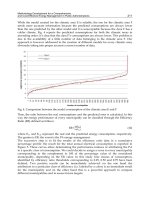
3.2 Experimental results
Figure 12 shows the relation of height h with lift and pull-off forces for specimens without
MEMS structures. The results for the specimens with MEMS structures are shown in Fig.13.
Experimental and calculated data are shown in (a) and (b), respectively, in both figures. In
the experiment, the supporting leg was first immersed gradually into water. In this process,

the lift force initially increased, reached a maximum, and then decreased slightly; finally, the
water’s surface was broken and the leg was completely submerged. After that, as the leg
was pulled out of the water, the leg remained submerged until it came close to the surface of
water. Then, a dimple of water formed abruptly, and it was gradually raised along with the
specimen. This hysteresis is observed in the experimental results shown in Figs 12 (a) and 13
(a), although this effect was not taken into account in the calculations.
The measured lift forces are in good agreement with the calculated values. The maximum
lift force depends on the diameter of the specimens rather than the surface properties of the
legs. The measured pull-off force decreases with increasing contact angle. This trend agrees
well with the theoretical predictions. However, the measurements for the values of the
maximum pull-off force and maximum height are smaller than those calculated. This is
because the meniscus bridge shrinks at one end of the leg and becomes a conical shape just
before the leg is completely pulled off. Therefore, a three dimensional dynamic model of the
meniscus is necessary to predict the maximum pull-off force quantitatively.
The PDMS hair-like structure wrapped on the wire of 0.5 mm in diameter enlarges to an
apparent diameter of 2.5 mm and increases the maximum possible lift force efficiently, even
though it does not improve the contact angle and pull-off force.

Bio-InspiredWaterStriderRobotswithMicrofabricatedFunctionalSurfaces 373

The third structure is formed on the surfaces of aluminium and brass wires by wet etching.
Figure 9 shows the process to fabricate the etched structures. First, photolithography on the
cylindrical metal wires was carried out in the same manner as in the SU8 structure. Here, a
positive type photoresist (Tokyo Ohka Kogyo, OFPR) was used instead of SU-8 (Fig. 9 (a)
(b)). The wires were then patterned by isotropic wet etching (Fig. 9 (c)), followed by removal
of the OFPR (Fig. 9 (d)). Finally, the same hydrophobic agent (FS-1010) was coated on the
structure. SEM photographs of the aluminium and brass structures are shown in Fig. 9 (e)
and (f), respectively. The brass structures have sharper edges than do the aluminium
structures.


4. MEASUREMENTS OF LIFT AND PULL-OFF FORCES

4.1 Experimental setup
To investigate the performance of the supporting legs, the lift and pull-off forces of the
fabricated legs were measured. The experimental setup for the measurements is illustrated
in Fig. 10. The geometry of the specimen is shown in Fig.11. Both ends of the specimen are
bent up in order to prevent the tip of the wire from breaking the water surface.
The surface of the water in a petri dish was moved vertically using a z stage to immerse and
pull out the specimen. The lift and pull-off forces were measured by using a laser
displacement sensor to detect the deformation of a parallel leaf spring fixed to the specimen.
By using two laser displacement sensors, the relative height of the specimen from the water
surface was also measured. Table I shows materials, surface structures, outer diameters, and
contact angles of the specimens. Three kinds of the hydrophobic-agent-coated specimens, as
well as four specimens with microfabricted structures on their surfaces, were prepared. The
contact angles of the microfabricated wires, except for the PDMS structure, increased by 5-10
degrees compared to those of the FS-1010 coated non-structured wire. The PDMS structure
was too large to show an increase in the contact angle.


Fig. 10. Experimental setup for measuring lift and pull-off forces


Fig. 11. Geometry of the specimen

Base wire
MEMS
structure
Hydrophobic
coating
Outer

Diameter
Contact
angle
Brass
φ
0.5

FS-6130
*1

0.5 mm
105°
Brass
φ
0.5

FS-1010
*1
0.5 mm
118°
Brass
φ
0.5

HIREC-1450
*2

0.62 mm
135°
Brass

φ
0.5
PDMS
FS-1010
*1
2.5 mm
117°
Brass
φ
1.0 SU-8
FS-1010
*1

1.1 mm
128°
Aluminium
φ
1.4
Etching
FS-1010
*1
1.4 mm 123°
Brass
φ
1.0 Etching
FS-1010
*1

1.0 mm
123°

*1 Fluoro Technology Corp. *2 NTT Advanced Technology Corp.
Table 1. Material, Diameter, and Contact Angle of the Specimens

3.2 Experimental results
Figure 12 shows the relation of height h with lift and pull-off forces for specimens without
MEMS structures. The results for the specimens with MEMS structures are shown in Fig.13.
Experimental and calculated data are shown in (a) and (b), respectively, in both figures. In
the experiment, the supporting leg was first immersed gradually into water. In this process,
the lift force initially increased, reached a maximum, and then decreased slightly; finally, the
water’s surface was broken and the leg was completely submerged. After that, as the leg
was pulled out of the water, the leg remained submerged until it came close to the surface of
water. Then, a dimple of water formed abruptly, and it was gradually raised along with the
specimen. This hysteresis is observed in the experimental results shown in Figs 12 (a) and 13
(a), although this effect was not taken into account in the calculations.
The measured lift forces are in good agreement with the calculated values. The maximum
lift force depends on the diameter of the specimens rather than the surface properties of the
legs. The measured pull-off force decreases with increasing contact angle. This trend agrees
well with the theoretical predictions. However, the measurements for the values of the
maximum pull-off force and maximum height are smaller than those calculated. This is
because the meniscus bridge shrinks at one end of the leg and becomes a conical shape just
before the leg is completely pulled off. Therefore, a three dimensional dynamic model of the
meniscus is necessary to predict the maximum pull-off force quantitatively.
The PDMS hair-like structure wrapped on the wire of 0.5 mm in diameter enlarges to an
apparent diameter of 2.5 mm and increases the maximum possible lift force efficiently, even
though it does not improve the contact angle and pull-off force.

Biomimetics,LearningfromNature374

Height [mm]
4

2
0
-2
-4
FS-6130 (105
o
0.5)
FS-1010 (118
o
0.5)
HIREC-1450
(135
o
0.62)
6
135
118
105
φ
0.5
φ
0.62
(Length: 30 mm)

(a) Experimental results
Height [mm]
105
o
φ
0.5

118
o
φ
0.5
135
o
φ
0.62
135
118
105
φ
0.5
φ
0.62

(b) Calculated results
Fig. 12. Lift and pull-off forces for hydrophobic-agent-coated legs



(a) Experimental results

(b) Calculated results
Fig. 13. Lift and pull-off forces for legs with microfabricated structures

5. DEVELOPMENT OF WATER STRIDER ROBOTS

5.1 Hexapedal robot
Two different mechanisms for surface-tension-based locomotion on the water surface were

developed. Figure 14 shows a hexapedal robot. The hydrophobic legs with PDMS hair-like
structures were used for the forelegs and hind legs to support the weight of the body. The
middle legs were attached to an actuating mechanism that creates the elliptical motion
required for propulsion. The resulting hexapedal locomotion is similar to that of an insect
water strider. Each supporting leg is 135 mm in length. From the results of Fig. 13 (a), the
loading capacity of the four supporting legs was predicted to be 138 mN (14 gf), which is
Bio-InspiredWaterStriderRobotswithMicrofabricatedFunctionalSurfaces 375

Height [mm]
4
2
0
-2
-4
FS-6130 (105
o
0.5)
FS-1010 (118
o
0.5)
HIREC-1450
(135
o
0.62)
6
135
118
105
φ
0.5

φ
0.62
(Length: 30 mm)

(a) Experimental results
Height [mm]
105
o
φ
0.5
118
o
φ
0.5
135
o
φ
0.62
135
118
105
φ
0.5
φ
0.62

(b) Calculated results
Fig. 12. Lift and pull-off forces for hydrophobic-agent-coated legs




(a) Experimental results

(b) Calculated results
Fig. 13. Lift and pull-off forces for legs with microfabricated structures

5. DEVELOPMENT OF WATER STRIDER ROBOTS

5.1 Hexapedal robot
Two different mechanisms for surface-tension-based locomotion on the water surface were
developed. Figure 14 shows a hexapedal robot. The hydrophobic legs with PDMS hair-like
structures were used for the forelegs and hind legs to support the weight of the body. The
middle legs were attached to an actuating mechanism that creates the elliptical motion
required for propulsion. The resulting hexapedal locomotion is similar to that of an insect
water strider. Each supporting leg is 135 mm in length. From the results of Fig. 13 (a), the
loading capacity of the four supporting legs was predicted to be 138 mN (14 gf), which is
Biomimetics,LearningfromNature376

sufficient to support a robot that weighs 5.4 gf. A DC motor and a lithium polymer battery
were mounted on the body, and non-tethered actuation was achieved.
The slider-crank mechanism, shown in Fig. 15, was used for creating the elliptical motion of
the middle legs. The trajectory of point P at the middle of the connecting rod is given by the
following equations:

2 2 2
cos 1 sin
sin
a
x r l r
l

a r
y
l
θ θ
θ

 
= + − −
 


 


=



(17)

Definitions of r, l, a,
θ
 and the calculated trajectory of P is shown in Fig. 16. Figure 17
illustrates the transmission mechanism for the middle leg. The 125-mm-long middle leg
penetrates the connecting rod at P and is supported at Q using a flexible ring, so that the
middle leg rotates conically around Q. The rowing angle of the leg is approximately 90
o
and
the elliptical motion of P is magnified by 10 at the tip of the leg.
The hexapedal robot was put on the surface of water in a container and the middle legs were

driven at 2 Hz. Forward motion was successfully achieved on the surface down to 5-mm-
deep water. The velocity determined from the images of a high-speed camera is shown in
Fig. 18 (a). A maximum speed of 90 mm/s and an average speed of 40 mm/s were achieved.
The middle legs were swept shallowly without breaking the surface of water and pulled off
during the power stroke. Consequently, deceleration starts in the middle of the power
stroke. Then, acceleration starts in the middle of the recovery stroke because of the inertial
force of the actuating legs. The velocity of an actual water strider obtained from high-speed
video images is shown in Fig.18 (b). The water strider accelerates all the way through the
power stroke and reaches a maximum speed of about 400 mm/s. Then it decelerates rapidly
in the recovery stroke. After that, it glides on the surface of the water, decelerating
moderately.


Fig. 14. Hexapedal water strider robot


Fig. 15. Slider-crank mechanism for creating elliptical motion of middle leg.


Fig. 16. Elliptical trajectory created by the slider-crank mechanism


Fig. 17. Structure of the middle leg
Bio-InspiredWaterStriderRobotswithMicrofabricatedFunctionalSurfaces 377

sufficient to support a robot that weighs 5.4 gf. A DC motor and a lithium polymer battery
were mounted on the body, and non-tethered actuation was achieved.
The slider-crank mechanism, shown in Fig. 15, was used for creating the elliptical motion of
the middle legs. The trajectory of point P at the middle of the connecting rod is given by the
following equations:


2 2 2
cos 1 sin
sin
a
x r l r
l
a r
y
l
θ θ
θ

 
= + − −
 


 


=



(17)

Definitions of r, l, a,
θ
 and the calculated trajectory of P is shown in Fig. 16. Figure 17

illustrates the transmission mechanism for the middle leg. The 125-mm-long middle leg
penetrates the connecting rod at P and is supported at Q using a flexible ring, so that the
middle leg rotates conically around Q. The rowing angle of the leg is approximately 90
o
and
the elliptical motion of P is magnified by 10 at the tip of the leg.
The hexapedal robot was put on the surface of water in a container and the middle legs were
driven at 2 Hz. Forward motion was successfully achieved on the surface down to 5-mm-
deep water. The velocity determined from the images of a high-speed camera is shown in
Fig. 18 (a). A maximum speed of 90 mm/s and an average speed of 40 mm/s were achieved.
The middle legs were swept shallowly without breaking the surface of water and pulled off
during the power stroke. Consequently, deceleration starts in the middle of the power
stroke. Then, acceleration starts in the middle of the recovery stroke because of the inertial
force of the actuating legs. The velocity of an actual water strider obtained from high-speed
video images is shown in Fig.18 (b). The water strider accelerates all the way through the
power stroke and reaches a maximum speed of about 400 mm/s. Then it decelerates rapidly
in the recovery stroke. After that, it glides on the surface of the water, decelerating
moderately.


Fig. 14. Hexapedal water strider robot


Fig. 15. Slider-crank mechanism for creating elliptical motion of middle leg.


Fig. 16. Elliptical trajectory created by the slider-crank mechanism


Fig. 17. Structure of the middle leg