20
Multiple Multi-Objective Servo Design -
Evolutionary Approach
Piotr Wozniak
Institute of Automatic Control, Technical University of Lodz
Poland
1. Introduction
Design of control systems is characterised by many targets, therefore the methods enabling
optimisation of several objectives have received more and more attention over the past
years. When dealing with multi-objective optimisation problems the notion of the scalar
function optimality was extended. The most common approach was originally proposed in
19th century by Edgeworth and later generalised by Pareto. This trade-off approach means
no element of the vector of optimal solution, so called Pareto optimal solution, can be
improved without making some other criteria worse. There are many different notions of
dominance. One of them is so called weak Pareto dominance relation which is defined as
follows :

(1)
where F ' is a set of objectives with

A solution x
*
∈ X is called Pareto optimal if there is no other x ∈ X that weakly dominates x
*

with respect to the set of all objectives taking into account all constraints. The set of all
optimal solutions form the Pareto set.
Most of the research in the multi-objective optimisation has concentrated on tracing
the Pareto front. Often this solution, which is non-dominated in the objective space, cannot
be described analytically especially when the complexity of the problem makes
exact methods unsuitable. The Pareto set is the projection of the Pareto front to the decision

space.
In the last 20 years meta-heuristics approach to the multi-objective optimisation problems
proved it can be applied even when only little is known about the underlying problems.
From these methods, evolutionary algorithms are, without a doubt, the most widely used
today mainly due to their flexibility while dealing with non-linear, non-quadratic, non-
convex problems and thanks to their ease of use (for extensive presentation of the state-of-
the-art research results see (Coello Coello, et al., 2007)). Also in engineering design
formulated as multi-objective optimisation problems the evolutionary algorithms (MOEA)
Automation and Robotics

344
achieve popularity (Fleming et al., 2005) although generating Pareto front approximation is
computationally expensive.
At the moment, thanks to rapid progress in computing technologies, novel algorithms of
population-based optimisation may now be run on multiprocessor computing platforms in
shorter time.
On the other hand, the designer, as well as the decision maker, may not be interested in
having an excessively large number of Pareto optimal solutions (vectors from the decision
space) to deal with due to overflow of information. Therefore, many multi-objective
optimisation problems are reformulated to find a manageable number of Pareto optimal
vectors which are evenly distributed along the Pareto front, and thus good representatives
of the entire set of decisions. In real problems, a single solution must be selected.
Preferably, unique solution must belong to the non-dominated solutions set and must take
into account the preferences of a designer and the decision maker.
Evolutionary methods are extensively applied for multi-objective optimisation problems
mostly with two or three objectives only (Coello Coello, et al., 2007). On the other hand
designers may prefer to put every performance index related to the problem as an objective,
rather than as a constraint, thereby increasing number of criteria. The problems with a high
number of objectives cause additional challenges with respect to low-dimensional problems.
Current algorithms, developed for problems with a low number of objectives, have

difficulties to find a good Pareto front approximation for higher dimensions. Even with the
availability of sufficient computing resources, some methods are practically not useable for
a high number of objectives. It has been investigated, whether it is possible to effectively
solve optimisation problems with a large number of objectives where most of solutions
generated become incomparable (Brockhoff & Zitzler, 2006). In the complex design it is
not clear whether any two given objectives are nonconflicting. That is, although a conflict
exists elsewhere, some objectives may behave in a non-conflicting manner near the Pareto
front. In such cases, the trade-off curve may be of dimension lower than the number of
objectives.
The problem of dimensionality reduction multi-objective optimisation is defined as
the question of finding a minimum objective subset, maintaining the given dominance
structure (1) and good approximation of the Pareto front.
There are increasing number of research recently on influence of the objectives reduction on
quality of the Pareto front approximation. In the literature dominates the a posteriori
approach, where reduction is performed after preliminary solution to the multi-objective
optimisation problems, (Deb & Saxena, 2005), (Brockhoff & Zitzler, 2006), (Woźniak, 2007a).
Alternatively, a reduction in the complexity of most design problems is typically achieved
by the problem decomposition based on the designer/decision maker’s knowledge
(Engau & Wiecek, 2007), or the transformation of the multi-objective optimisation problem
into the set of single-objective optimisation problems (Qingfu & Hui, 2007).
The objective of this study is twofold. First, aim is to find a new coordination mechanism
which guarantees that the final selection leads to a design that is Pareto optimal for
the overall multiple Multi-Objective Optimisation Problem (mMOOP). The second aim is
to propose a procedure for the mMOOP with many objectives solution under the changing
environment conditions.
The methodology presented in this study integrates several multi-objective optimisation
problems, while steering clear of the high dimensionality problems.
Multiple Multi-Objective Servo Design - Evolutionary Approach

345

The issues of multi-objective optimisation are highlighted in Section 2. The multiple multi-
objective optimisation problem is outlined in Section 3 while the proposed algorithm for the
mMOOP solution is proposed in Section4. In Section 5 the application of the mMOOP
design is presented for the servo design as a future field of interest. The Section 6
summarizes the study.
2. Dimensionality issues in multi-objective optimisation
The majority of the existing multi-objective evolutionary algorithms for approximating
the Pareto front have been designed for, and tested on, low dimensional examples (Coello
Coello, et al. 2007). However, for complex optimisation problems often a higher number
of dimensions occur. Increased number of criteria cause difficulties in terms of the quality of
the Pareto front approximation and running time (e.g. algorithms based on
the hypervolume indicator (Brockhoff & Zitzler, 2006) lead to running times exponential in
the number of objectives). Additionally there is a greater probability of having any two
arbitrary solutions to be non-dominated to each other. Consequently the proportion of such
solutions in the population increases. Since multi-objective evolutionary algorithms put
more emphasis on the non-dominated solutions, a significant part of the old population is
preserved in the elite (Coello Coello, 2007). Therefore growing elite leaves no much room for
new solutions to be included in the population when the constant size of pool is assumed.
This, in consequence, reduces the selection pressure for the better solutions in
the population and the search process slows down.
When the Pareto dominance-based ranking procedures become ineffective determining
the quality of solutions, new measures and relations are introduced to guide
the optimisation process. Recent results on using preference order-based approach as
an optimality criterion in the ranking stage of multi-objective evolutionary algorithms
(Engau & Wiecek, 2007) proved convergence improvement.
In general dimension reduction aims at keeping those objectives that can explain most of
the variance in the objective space. However, it is not clear :
i. how the objective reduction alters the dominance structure,
ii. what is the quality of a generated objective subset.
The most accepted method is aggregation of the vector objectives into the single criterion by

introducing the weighted sums. The multi-objective problem is therefore reduced to single
function optimisation which is easy to solve even in the presence of local optima and, on
a first sight, scale well.
But for high dimensions these techniques reach their limits, since :
i. it is hard (or even impossible) to determine good weights,
ii. such approaches lack the desired parallel search ability.
Another prospective ways of solving this type of problems includes reduction in the number
of objectives (Brockhoff & Zitzler, 2006), (Woźniak & Witczak, 2007), (Woźniak, 2007a) or
discovering objectives, which are entirely unrelated by the divide-and-conquer strategy
(Purshouse & Fleming, 2003). The later method is based on splitting multi-objective
optimisation problem into sub-problems. The main limitation of this approach is excessive
number of pair-wise comparisons at the merge step after solution of sub-problems.
Decomposition methods are particularly well suited for design optimisation as most of
complex engineering systems usually consist of many subsystems and components having
smaller complexity. Dividing large and complex systems into several smaller entities is done
Automation and Robotics

346
to enable local optimisation and decision-making. In general, however, these subsystems
will still be coupled so that the solution of each subsystem is dependent upon information
from the others. Hence, along with the benefit of reduced complexity, comes the issue of
exchange of the separate design decisions (i.e. values of the criteria arguments) to eventually
arrive at a single overall design solution that is feasible. To solve this coordination problems
the concept of the multiple multi-objective optimisation is introduced in Section 3.
3. Problem definition
The mathematical background of the multiple multi-objective optimisation problem remains
the same as of a classic multi-objective optimisation problem.
We consider the common formulation of the multi-objective optimisation problem in its
general form :


[]
12
12
. (),
[, , , ],
() (), (), , () ; 2
min
s.t.
m
m
n
fx
xxx x
xX S R
fx f x f x f x n
=
∈⊆⊆
=
≥
…
…
(2)
[
]
[]
12
12
. () (), (), , () 0,
() (), (), , () 0,
m

l
gx g x g x g x
hx h x h x h x
=
≤
==
…
…
subject to

where x is the vector of the decision variable, which might be subject to inequality g(x)
and/or equality constraints h(x).
A solution which satisfies all the constraints is called a feasible one. Due to contradicting
objectives there is no single solution to (2). Instead there is a set of alternative solutions.


Fig. 1. Representation of the decision space and the corresponding objective space.
These solutions are optimal in the sense that no other solutions dominate (are superior to)
them when all objectives are considered. They are known as Pareto-optimal solutions.
The interest, in the classical multi-objective optimisation problem, is therefore on the trade-
offs with respect to the objectives (Shukla & Deb, 2007). Each objective function maps
Multiple Multi-Objective Servo Design - Evolutionary Approach

347
the input decision vector (point in the m dimensional decision space) (see Fig. 1) to
the target vector in the n dimensional objective space.
The domination relation defined in the objective space is used to identify
i. the Pareto set in the decision space,
ii. the Pareto front in objective space and
iii. the Pareto rank of each solution.

The main difference between approach introduced in this study and classical single multi-
objective optimisation problem lies in the synchronised consideration of simultaneous
multi-objective optimisation problems sharing the same decision space, but with
the environment changes. Distinct environment conditions may be introduced when
variations in the multi-objective optimisation problem formulation is needed to describe
discrepancy between the physical plant and the mathematical model with constraints used
for the design.
Every vector of the environment changes form the context which therefore is identified by
its parameters, and is denoted c. The context belongs to the permissible environment
conditions space C
o
.
There are several possible ways to integrate environment conditions c
∈
C
o
into a classical
multi-objective optimisation problem. In each case the vector of objective functions (results
in Fig.2) changes.

Fig. 2. The changes of environment conditions for the plant leading to multiple multi-
objective optimisation problem (mMOOP).
The alternatives may be obtained by :
i. extending the decision (input) vector by the context c. Now we consider the resulting
mapping with extended (comparing to (2)) arguments f*(x,c) . A common algorithm for
a multi-objective optimisation problem is used to find all optimal solutions in
the decision space of the higher dimension. Since the decision space of the problem and
the context space C
o
are unified, just the optimal solutions x

*
c
over the new input space
will be found. For this reason such integration of the environment conditions is not
suitable for the control system design.
ii. extending the objective vector by the context c. The resulting mapping will be f
c
(x) with
f
c
∈ FC
n+o
in higher dimensional space. A common algorithm for a single multi-objective
optimisation problem is used to find all optimal solutions in the objective space of
the higher dimension. For this reason, as discussed in details in Section 3, such
an integration of the context is not preferred.
context
results
decisions
mMOO
evolu-
tionary
framework
Automation and Robotics

348
iii. treating every context as a single multi-objective optimisation problem.
This corresponds to an exhaustive a-posteriori search in every o approximated Pareto
fronts (for all possible contexts). It is obvious that such an approach is not efficient,
because it leads to optimisation in the set of o fronts f

c
(x
c
).
iv. The multiple multi-objective optimisation problem mapping. The characteristic is that
all different multi-objective optimisation problems share the input space, and the
outputs are generated concurrently f
c
(x).
The key observation is that in the multi-objective optimisation problem framework iv.
finding Pareto optimal solutions is equivalent to a search for a trade-off solution with
variation within some parameters.
In this study variations included in the multiple multi-objective optimisation problem
mapping formulation iv. are considered as distinct working conditions of the system (see
Fig.2).
Directly from the above definitions of the multiple multi-objective optimisation problem
mapping follows that there are multiple outputs for a single decision input (one for every
context). After collecting a set of solutions, the Pareto rank for every solution in each context
can be calculated.
To compress this information to a single value only the highest Pareto rank value
(the lowest from the calculated
i
c
Prank ) is selected and further defined as

{
}
,,,
12 o
cc c

bPrank = min Prank Prank Prank…
(3)
This value bundles the quality of a solution into a single value. As a result its value is crucial
for multi-objective optimisation algorithms, because they are based on ranking comparisons
of different solutions.


Fig. 3 Multi-objective control design framework with task requirements - context.
In this work, we propose a procedure of transferring some performance criteria of
the control system into the context variables. The approach is motivated by the real-life
problem of having a large number of potential objectives in the redundant robot
manipulators control based upon the existing multi-criteria inverse kinematics, and will be
discussed in details in Section 5.
The task-based controller is a controller that unifies position and force control of redundant
manipulators and takes task requirements as the central component of the multi-objective
control design framework, with context presented in Fig. 3.
Goal-based objectives
and performance

Control
g
oals
Context (task requirements)
Multi-ob
j
ective desi
g
n
Multiple Multi-Objective Servo Design - Evolutionary Approach


349
4. Evolutionary methodology of the multiple multi-objective optimisation
problem solution
Since evolutionary algorithms deal with a number of population members in each
generation, they are ideal for finding multiple Pareto-optimal solutions in of the multi-
objective optimisation problem. All of these methods emphasize :
i. non-dominated solutions for progressing towards the Pareto-optimal front,
ii. less-crowded solutions for maintaining a good diversity among obtained solutions,
iii. elites to provide a faster and reliable convergence near the Pareto-optimal front.
There are numerous approaches for solving multi-objective optimisation problems.
The salient features of multi-objective evolutionary algorithms are :
i. the convergence of solutions in the objective space to the Pareto front,
ii. support for diversity of the solutions along the front,
iii. efficiency characterised by the processing time or the number of evaluations
required.
New algorithms introduced every year aim to improve on one or more of the above
mentioned issue. Some of the most well-known algorithms are: VEGA, MOGA, PAES,
NSGA-II and SPEA2. For comprehensive description see (Konak et al., 2006) and (Coello
Coello et al., 2007).
Essential parameters to be fixed in an evolutionary algorithm:
i. population size,
ii. number of generations,
iii. parameters related to selection,
iv. recombination (crossover probability, crossover operator),
v. mutation (mutation probability, mutation operator).
Population size is a crucial parameter in a successful application of each algorithm. Even in
the case of an adequate population size optimisation the algorithm must be run for a critical
number of generations in order to obtain convergence near the optimal solution (Coello
Coello et al., 2007).
In case where context can be configured concurrently, a single evaluation run delivers

several results, each consisting of multiple objective values, for each instance of the multi-
objective optimisation problem.
The presented approach is based on sequential calculations of MOO sub-problems of
the multiple multi-objective optimisation problem. After selecting one, leading multi-
objective optimisation problem, its Pareto set is henceforth considered as constant for all
remaining multi-objective optimisation problems.
The idea behind this approach is presented in Fig. 4 for two contexts of a bi-objective
problem (denoted f
1
1
f
2
1
in Fig. 4a and f
1
2
f
2
2
in Figs. 4b and 4c, respectively).
After four elements of the Pareto front for the first context are found and designated with
different symbols in Fig. 4a, their arguments in the decision space are passed to the second
context. Using each of the values may result in a front shown in Fig. 4b, when the next,
second, multi-objective optimisation problem is solved. This means that for each point in
the objective space of the first multi-objective optimisation problem there may be more than
one solution in the second objective space. These are designated by the same symbols like in
Fig. 4a.
In the next step the results are sorted for non-dominancy and lead to the front depicted in
Fig. 4c (dominated solutions are discarded).
Automation and Robotics


350

Fig. 4 Outline of Pareto front derivation for two contexts of bi-objective optimisation
problems
Considering the above mentioned approach, the pseudo-code of the proposed sequential
optimisation may be formulated as presented in Fig. 5.
For this specific multiple multi-objective optimisation problem design the order of
the considered sequences of contexts is far less important than in the similar multiple multi-
objective optimisation problem s proposed in (Avigad, 2007) and (Ponweiser &
Vincze, 2007). It is possible to make it robust to the order of the multi-objective optimisation
Multiple Multi-Objective Servo Design - Evolutionary Approach

351
problems by introducing epsilon tolerances to reflect the implicit trade-off between
solutions of two different contexts.

1. Decision Making step - identify all contexts
c
i
, i=1, ,o, and introduce the order in the C
set.
2. Initialise parameters of MOEA and search space.
3. Apply MOEA with non-dominated sorting to solve
C
1
. Store results in form of the Pareto set x
1

and the Pareto front c

1
, i.e. (x
1
,t
1
).
4. For j:= i+1 to o do
a. Initialise c
j
th
MOEA parameters taking into
account Pareto solutions (x
j-1
,c
j-1
)
b. Apply MOEA with non-dominated sorting to
solve c
j
. Store results in form of
the Pareto set x
j
and the Pareto front c
j
,
i.e. (x
j
,c
j
)

c. Reject from (x
j-1
,c
j-1
) solutions, which
became dominated in the j
th
step
5. IF the maximal number of populations is reached
THEN STOP ELSE goto STEP 3
Fig. 5 Pseudo-code of the proposed mMOOP algorithm.
Solving the individual MOO sub-problems before selecting a final design generally may
overemphasize one context, while significantly degrading the performances of others.
Moreover, it is shown that the best compromise solution is not necessarily optimal for any
MOO sub-problem, and thus remains unknown to the designer who follows the traditional
decomposition – integration approach. We plan to consider this issue in the near future.
The first and probably the most important property that needs to be considered for
the design of optimiser for a multiple multi-objective optimisation problem are multiple
instances of the objective space. There exists one for every context. Although any of
averaging technique can be used to operate in these spaces (e.g. mean, standard deviation,
minimum or maximum value), a careful selection of values from each one is needed.
Furthermore, the computational effort increases enormously because the calculations have
to be done for every context separately. Out of these insights it is advisable to avoid
performing any operations in the objective space.
In classical multi-objective evolutionary algorithms methods the objective space is
intuitively used to calculate the density of solutions (for example in SPEA2 or NSGA-II).
A solution for the multiple multi-objective optimisation problem is to relocate the density
calculations from the objective space to the decision space. The placement of these measures,
either in the decision space or in the objective space, was subject to a long scientific
discussion (Coello Coello et al., 2007). In most of the implementations the objective space is

used. Therefore, at this stage of research on multiple multi-objective optimisation problem,
the NSGA-II (Deb, 2001) state-of-art algorithm is considered as the most prospective.
Automation and Robotics

352
Another effect that needs to be considered is the extension of the Pareto rank to the best
Pareto rank (3). In the NSGA-II the Pareto rank is the main selection criteria. A drawback of
the best Pareto rank is its computational effort, but so far no better approach may be put
forward. The complexity of a single Pareto rank calculation is multiplied by the number
of contexts. This issue still lacks a computationally effective solution.
5. Multiple multi-objective optimisation problem of servo control - an outline
We will consider the so-called mechatronic servo system, i.e. the servo system adopted in
the numerical control machine or industrial robot with many joints. Generally, dynamic
characteristics of robot actuators and sensors are highly nonlinear with constraints, and
these factors cause trajectory control errors. Feeding back the difference between the robot
servomechanism velocities enables force adjustment.
The performance criteria for robot control optimisation may be broadly divided into two
categories :
i. constraint-based criteria,
ii. operational goal-based criteria.
The constraint-based criteria, as its name implies, are directly associated with system
constraints (e.g. joint limits, obstacles, singularities, etc.). Therefore, in general they have
clear physical meanings that the user can easily relate to. They are task-dependent and
usually give more insight to the operator on the task at hand.
Operational goal-based criteria, on the other hand, are concerned with the ability of
the robot to perform the task better. They are functions of only manipulator configuration
and states, and are not tied to any specific task. This makes the criteria very useful for
the system designer, who cannot foresee all the possible tasks the robot could perform in
the future.
The comprehensive description of the objectives, and performance criteria, for optimisation

of redundant robot system presented hereafter was published in the Ph.D. thesis (Pholsiri,
2004). Redundancy, in this context, is defined as having more inputs than those required
to create the desired output. As such, traditionally non-redundant robots, e.g. most
6 degrees of freedom (DOF) commercial robots, can be considered redundant too if their
tasks at hand require fewer DOFs than the robots possess. Redundancy implies an ability
to change configuration of the joint without changing the position of the robot’s
end-effector.
The main criteria are listed hereafter, and will enable the introduction and formulation of
the multiple multi-objective optimisation problem :
C1 Criteria for Joint Range Availability (JRA).
Every joint in a manipulator has its travel limits which cannot be exceeded. Any attempt
to move a joint over its limit can potentially damage the robot.

,
1
,
1
mid
max
θθ
γ
θ
=
⎛⎞
−
⎜⎟
=
⎜⎟
⎝⎠
∑

p
n
ii
JRA
i
i
n
(4)
where :
θ
i
is the joint displacement,
θ
i,mid
is the displacement at the midpoint of the travel range,
θ
i,max
is the displacement at the travel limits.
Multiple Multi-Objective Servo Design - Evolutionary Approach

353
C2 Criteria for Velocity Limit Avoidance.
The joint Velocity Limit Avoidance (VLA) tries to minimise the velocity of each joint or
the sum of the velocities of all joints. The velocity limit can be avoided by minimizing
the norm of the joint velocity vector. It is crucial to keep VLA from approaching 0.
The pseudo inverse solution minimises the VLA criterion.
C3 Criteria for Peak Torque Avoidance.
Although their formulation is simple and straightforward, their use in practice is limited for
various reasons. First of all, the torque readings require that torque sensors be present at all
actuators, which is not common (due to their cost). Secondly, even with the torque

information available, this criterion can only be used to monitor the torque states of
the robot but generally cannot be used in redundancy resolution to prevent the robot from
exceeding their joint torque limits because most, if not all, redundancy resolution techniques
do not work in the force domain.
C4 Criteria for Obstacle Avoidance.
When a manipulator is utilised in a cluttered environment or in a multi-arm system,
the need to avoid obstacles or contacts with other manipulators arises. This may be
formulated in the form that it is independent of the number of links and the number of
obstacles.
C5 Criteria for Mathematical Singularity Avoidance.
Physically, at singularities, a manipulator loses one or more degrees of freedom. The robot
may not be able to move along the desired direction. To avoid mathematical software
failure, it is crucial to keep MSA from approaching zero.
The objectives mentioned above (C1 - C5) represent constraint-based criteria and may
compose the context for operational goal-based objectives (Gi).
The most important goal-based objectives are :
G1 Criteria for Manipulator Precision.
A manipulator’s joints are expected to have some amount of error, including position sensor
error (encoder resolution or noise), control error, and deflection due to joint compliance.
These joint errors are propagated through the links and to the end effector. Minimizing
the effect of this error propagation is essential in applications requiring precise
manipulation.
G2 Criteria for Speed of Operation.
Maximising Velocity Transmission Ratio (VTR) will minimise the joint velocity required
to produce a given end effector speed in the direction, in general or for any given joint
velocity.
G3 Criteria for Load Carrying Capacity.
Maximizing Force Transmission Ratio (FTR) will increase the end effector force capability in
the desired direction. Looking at formulations of the VTR and the FTR, it can be concluded
that they are not independent.

G4 Criteria for Energy Minimisation.
Kinetic energy minimisation is one of the early criteria used in redundancy resolution
because kinetic energy is directly associated with the power consumed by the system during
its operation. It is desirable to minimise the energy-based objective, especially for repetitive
tasks.
Automation and Robotics

354
A quick look at the list of performance criteria (G1 - G4) reveals that most, if not all, of these
criteria are coupled. It is therefore not possible to optimise one criterion without affecting
another. Hereafter there is a list of the major interaction between criteria. For example,
maximising the JRA (4) criterion will likely have an impact on the VTR criterion. Even
though the intention of adding the JRA to the redundancy resolution process is merely
to avoid the joint limits, we may unintentionally decrease the ability of the robot to move in
a desired direction. These couplings also make it impossible to completely separate
the purposes of these criteria, making the task of choosing criteria for a given optimisation
very difficult.
These couplings result in conflicts among criteria. The best example is the conflict between
the speed and force capabilities of the robot. When considering them independently one
would like to maximise both of them. However, because of the conflicting nature of these
two quantities, it is physically impossible to do so at the same time. A closer look at the VTR
and the FTR criteria shows that these two criteria are tightly coupled. As a matter of fact in
some special cases they are the reciprocals of each other. It was investigated whether
the VTR can be used to either increase the end effector speed or the end effector precision
(Pholsiri, 2004). However, while increasing the speed requires that VTR be increased,
improving the end effector precision demands the opposite.
These conflicts also cause difficulty when choosing appropriate criteria for a given task.
The problems of couplings and conflicts among performance criteria are one of the main
motivations behind the multi-objective optimisation research in the robot’s servo control
design.

In the considered redundant robot control problem the context is defined by constraint-
based criteria (C1-C5).
While it is essential to keep the system from violating constraints (C1-C5) during operation,
their values are not objectives of optimisation. Instead, their values may differ from one
context to another. The most straightforward approximation is to keep every constraint
constant during optimisation in each context.
At the present moment the investigation on the proposed novel multiple multi-objective
optimisation problem is at its early stage of development. First simulation experiments
showed that there is still significant potential for improvement, especially in
the development of metrics measuring the performance of optimisation algorithms for
multiple multi-objective optimisation problem in decision space, instead of using evaluation
in the objective spaces (one space per context).
5. Case study – servo design
The mechatronic servo system, i.e. the servo system adopted in the numerical control
machine or industrial robot is considered. In this system, there are two types of control.
One is position control (PTP: point to point) emphasizing the arriving time and stop position
from any position without considering the response route. Another is the contour control
emphasizing the motion trajectory from the current position to the next position (position at
each moment and its motion velocity).
The typical system includes the servo system of each axis, which is consists of the following
parts :
Multiple Multi-Objective Servo Design - Evolutionary Approach

355
− the motor ,
− the power amplifier ,
− the current control ,
− the velocity control ,
− the position control.
The structure of the system is generally different from the servo system introduced in

textbooks of automatic control and is presented in Fig. 5 (Woźniak, 2007b).


Fig. 5. Mechatronic servo system structure
5.1 The comprehensive presentation of three multi-objective problems
The overall design problem may be considered mMOOP with divided into three MOOPs as
outlined in Fig.6.


Fig. 6 The epsilon tolerance integration of the mMOOP with distinct contexts
The control goals may be easily organised in the same manner as presented in Fig.5. It is
realistic, from engineering point of view, to consider position control part of the design as
the most important one. This loop is responsible for the following the reference path with at
last two conflicting targets - fast transients and small overshoot combined with the zeroing
steady-state error. The position control loop supervises velocity signal control.
The dynamics of this subsystem also has at least two conflicting objectives.
Automation and Robotics

356
The most inner part of the presented in Fig. 5 servo system structure has the most complex
dynamics forced by the pulse-width modulation control of the permanent magnet
synchronous motor. Unlike the mechanical control loops(i.e. Velocity signal, and Position
signal), this one has to be modeled by discrete-time model with time constants of several
microseconds.
The mMOOP interaction between multi-objective designs takes into account some
tolerance ε, which improves robustness of the solution (Engau & Wiecek, 2007) and is
realised according to the coordination scheme outlined in Section 4 (see Fig.4).
6. Conclusions
This study contributed a novel formulation to the emerging research area of
the optimisation methods - the multiple multi-objective optimisation problem. It is

an extension of the multi-objective optimisation ideas to the set of concurrent multi-objective
optimisation problems defined by changing the environment conditions - the context.
In this study, the burden of high dimensional multi-objective optimisation problem (as
discussed in Sect. 3) is relaxed by considering aggregation of the constraint-based criteria
with conditions for operational goal-based objectives.
The Pareto optimal solutions of the multiple multi-objective optimisation problem are
evaluated without introducing ordering of the multi-objective optimisation problems.
The shared decision space of multi-objective optimisation problems is considered as
a connecting bridge between all multi-objective optimisation problems.
As an example from the control servo system design, the redundant robot design problem is
outlined for further research.
In the future work, we intend to further investigate the information that can be obtained
from the proposed trade-off and sensitivity analysis. In view of the current approach, we are
aware of the remaining weakness that this information only allows a local trade-off
assessment, and thus cannot be used for more accurate estimates in a larger region of
the outcome space.
We would also like to address remaining issues such as computational benchmarking or
further analysis of effects from grouping and ordering of objectives using examples from
the industry. We believe that such future efforts will further improve the recognised
features of the current method and eventually provide an effective and flexible decision-
making tool for multi-objective design optimisation.
7. References
Avigad, G. (2007). multi-Multi-Objective Optimization Problem and Its Solution by
a MOEA, Proceedings of the 4th Conference on Evolutionary Multi-Criterion
Optimization - EMO 2007, Obayashi S. et al. (Eds.), pp.847–861, ISBN 978-3-540-
70927-5, Matsushima, Japan, March 5-8, 2007, Springer, Berlin
Brockhoff, D. & Zitzler E. (2006). Are All Objectives Necessary? On Dimensionality
Reduction in Evolutionary Multiobjective Optimization, Proceedings of the 9th
Conference on Parallel Problem Solving from Nature-PPSN IX, Runarsson, T.P. et al.
Multiple Multi-Objective Servo Design - Evolutionary Approach


357
(Eds.), pp. 533–542, ISBN 978-3-540-38990-3, Reykjavik, Iceland, September 9-13
2006
Coello Coello, C.A. ; Lamont, G.B. & Van Valdhuizen, D.A. (2007). Evolutionary Algorithms
for Solving Multi-Objective Problems (2
nd
Ed.), ISBN 978-0-387-332549-3, Springer,
Berlin
Deb, K. (2001) Multi-Objective Optimization Using Evolutionary Algorithms, Wiley, ISBN 978-0-
471-87339-6, Chicester, UK
Deb, K. & Saxena, D.K. (2005) On finding pareto-optimal solutions through dimensionality
reduction for certain large-dimensional multi-objective optimization problems.
Technical Report KanGAL Report No. 2005011, Kanpur Genetic Algorithms
Laboratory, 2005
Engau, A. & Wiecek, M.M. (2007). 2D decision-making for multicriteria design optimization,
Structural and Multidisciplinary Optimization, Vol.34, No.4, (Oct. 2007), pp. 301-315,
ISSN 1615-147X
Fleming, P. J.; Purshouse, R. C. & Lygoe, R. J. (2005). Many-Objective Optimization:An
Engineering Design Perspective, Proceedings of the 3rd. Conference on Evolutionary
Multi-Criterion Optimization - EMO 2005, Coello Coello, C. A. et al. (Eds.), pp. 14–32,
ISSN 0302-9743 Guanajuato, Mexico, March 2005
Konak, A. ; Coit, D.W. & Smith, A.E. (2006). Multi-objective optimization using genetic
algorithms: A tutorial, Reliability Engineering and System Safety, Vol.91, pp.992-1007,
Sept.2006
Pholsiri, C. (2004). Task-based decision making and control of robotic manipulators
Ph.D. Thesis, University of Texas at Austin, 2004, Available at :

Ponweiser, W. & Vincze, M. (2007) “The Multiple Multi Objective Problem - Definition,
Solution and Evaluation, Proceedings of the 4th Conference on Evolutionary Multi-

Criterion Optimization - EMO 2007, Obayashi, S. et al. (Eds.), pp. 877–892, ISBN 978-
3-540-70927-5, Matsushima, Japan, March 5-8, 2007, Springer, Berlin
Purshouse, R. C. & Fleming, P. J. (2003) An adaptive divide-and-conquer methodology for
evolutionary multi-criterion optimisation, Proceedings of the 2nd Conference on
Evolutionary Multi-Criterion Optimization EMO 2003, Fonseca, C.M. et al. (Eds.),
pp. 133–147, ISBN 978-3-540-01869-8, Faro, Portugal, April 8–11, 2003, Springer,
Berlin
Qingfu, Z. & Hui, L. (2007) MOEA/D: A Multiobjective Evolutionary Algorithm Based on
Decomposition, IEEE Trans on Evolutionary Computation, Vol. 11, No. 6, (Dec. 2007),
pp.712-731, ISSN 1089-778X
Shukla, P.K. & Deb, K. (2007) On finding multiple Pareto-optimal solutions using classical
and evolutionary generating methods, European Journal of Operational Research,
Vol.181, No. 3, (Sept 2007), pp.1630-1652, ISSN 0377-2217
Woźniak, P. (2007a) Dimensionality Reduction in Evolutionary Multiobjective Design: Case
Study, Proceedings of the 9th annual conference on Genetic and evolutionary computation
GECCO-2007, Thierens et al. (Eds.), pp. 913-915, ISBN 978-1-59593-697-4
Woźniak, P. (2007b) Multiple Multi-Objective Optimisation of Servomechanism Control
Systems Design - Evolutionary Approach, Proceedings of the 13th IEEE International
Automation and Robotics

358
Conference on Methods and Models in Automation and Robotics MMAR
2007, Emirsajłow, Z. (Ed.), pp. 379-385, Szczecin, Poland, August 27-30, 2007
Woźniak, P. & Witczak, P. (2007). Dimensionality Reduction in Evolutionary Multiobjective
Design of Permanent Magnet Generator, Proceedings of the 4th Conference on
Evolutionary Multi-Criterion Optimization EMO 2007, Obayashi S. et al. (Ed.),
pp. 63-68, LBP, Matsushima, Japan, March 5-8, 2007
21
Model-Based Control of a Nonlinear One
Dimensional Magnetic Levitation with a

Permanent-Magnet Object
Zhenyu Yang, Gerulf K.M. Pedersen and Jørgen H. Pedersen
Esbjerg Institute of Technology, Aalborg University
Denmark
1. Introduction
The Electromagnet levitation technique has been popularly used in transport and industrial
felds in recent decades, such as high-speed levitation trains, frictionless magnetic bearings,
and high precision control in semiconductor manufacturing (CST (1996); Kim et al. (1998)).
Due to its high efficiency and good environmental orientation, the application of this
technique is extensively growing. For instance, the attitude of a small-sized satellite can be
efficiently controlled by using the electromagnetic force generated from the interaction
between the on- board (controlled) electrical field and the earth magnetic field (Wisniewski
& Stoustrup (2004)).


(a) Conventional structure (b) Considered structure
Fig. 1. Principles of conventional and considered levitation systems
The principle of electromagnetic levitation can be illustrated by a simple one-dimensional
system as shown in Fig.1 (a). By controlling the electric current flowing through coils
around a solenoid, a conductible object, e.g., an iron or a steel ball, can be possibly levitated
by the generated magnetic force. However, to develop a reliable and efficient levitation
system is far from easy with respect to the fact that this kind of system is featured by
Automation and Robotics

360
complexity, nonlinearities, natural instability and large electromagnetic uncertainties
(Gentili & Marconi (2003); Kim (1997); Thompson (2000); Varella et al. (2004)).
A planar levitation system was investigated in (Kim (1997); Kim et al. (1998); Thompson
(2000)). By conducting AC current through a disk-shaped insulated coil, the coil can be lift-
off above a wide aluminum plate. The realized system is stable but under-damped without

feedback control. The thermal problem is also investigated in (Thompson (2000)), and it
turned out that the coil resistance increased significantly with the increase of temperature,
which means that the system required more power in order to keep the levitated object at
the same height when the temperature increases. As a consequence, the test setup can only
be run for a few second at a time (Thompson (2000)). In order to control the levitated object's
position and overcome the under-damping issue, a feedback mechanism is often required.
The feedback control of a laboratory-sized one-dimensional levitation system is discussed in
(Wong (1986)), and an analog lead compensator was developed using standard frequency
response methods. Some application of advanced control methods such as the robust control
and integrator back- stepping for magnetic bearing control can be found in (CST (1996)) and
references therein. As we observed that most existing controllers are designed based on
some kind of linear/linearized models and therefore linear. Measurements of the levitated
object position and the current through the coil are often required by these controllers.
By focusing on the one-dimensional levitation, the comparison of system performances
under a linear controller and a nonlinear controller was investigated in (Barie & Chiasson
(1996)). The nonlinear controller was developed by using feedback linearization based on a
nonlinear model (Isidori (1989)). It showed that both controllers resulted more or less same
system performances in terms of tracking capability for step-type references. However, the
nonlinear controller is more sensitive to quantization error (e.g., 8 bit or 12 bit A/D
convertors) in the current measurement. Regarding the sinusoid-type references, it turned
out that the nonlinear controller resulted much better tracking performance than the linear
controller did. However, the development of nonlinear controller heavily depends on the
precision of available mathematical model. From practice point of view, no matter what
kind of controller will be used, the thermal dynamic (heating coil) is always a critical
concerning issue (Sønderskov & Østerö (2007); Thompson (2000); Yang & Pedersen (2006);
Yang et al. (2007)).
Different from most existing one-dimensional levitation systems which use a conductible
ball or coil as the levitated object (Barie & Chiasson (1996); Gentili & Marconi (2003);
Oliveira et al. (1999); Wong (1986); Yang & Pedersen (2006), here we consider a one-
dimensional levitation system with a permanent magnet object instead, i.e., a small NIB

(Neodymium, Iron, Boron) magnet is glued at the inside top of a plastic ball as shown in
Fig.0 (b). The main benefits of this configuration lie in the following perspectives:
• The solenoid's overheating problem is moderated. It is known that a large magnetic
field is often required to levite a conductible object even with a relatively small
operating range. It means that the coils must provide a large amount of current which
directly leads to the heat dissipation problem (Thompson (2000)). Instead of purely
depending on the coils, the magnetic field generated in the proposed configuration
consists of contributions from the permanent NIB magnet as well as the contribution
from coils around the solenoid.
• The system's operating range is enlarged under the same solenoid condition compared
with the standard configuration (with conductible object). The magnetic field is
Model-Based Control of a Nonlinear One Dimensional Magnetic Levitation with
a Permanent-Magnet Object

361
considerably enhanced due to the contribution from the NIB magnet. In our constructed
system the NIB contributes 4-5 times more flux density than the solenoid operating at
the maximal current (Sønderskov & Østerö (2007); Yang et al. (2007)).
However, the payoff of the above benefits is the complexity. The proposed configuration
makes modeling and control of this kind of levitation system much more complicated
regarding the fact that a permanent magnet is attached on a moving object (Simpson (1999)).
This paper will explore the modeling, control and implementation of the proposed levitation
system. First of all, the magnetic field generated by the moving NIB is experimentally
investigated and modeled. Then a nonlinear model of the entire system is derived. System
parameters are identified using some experimental ways. Afterwards a set of PID controllers
are designed via trial-and-error method and automatic tuning using genetic algorithms,
respectively. The developed controllers are implemented in the PC-supported LabView
environment. The experimental tests show some good system performances. The rest of the
paper is organized as: Section 2 gives a brief description of our benchmark system; Section 3
derives the nonlinear model of the considered system and then identifies the system

coefficients by experiments; Section 4 analyzes the PID control design, automatic tuning and
implementation issues; Section 5 discusses experimental results and we conclude the paper
in Section 6.
2. Experimental apparatus
A one-dimensional levitation system is constructed using an aluminium framework as
shown in Fig. 2. The electromagnet device consists of a solenoid with an iron core which is
composed of thin steel plates riveted together. The levitated object is a plastic ball with
diameter of 2 cm. There is a small NIB magnet glued to the top inside the ball, and a M4 nut
glued to the bottom acting as the counterweight to the NIB magnet. On the sides of the
framework, slits are milled for ease of mounting and adjustment of the optical sensor
system.


Fig. 2. Experimental laboratory setup
2.1 Position sensor
An optical sensor system for measuring the distance between the solenoid bottom and the
levitated ball is developed using two LEDs (IR333-A) and a photodiode array (Hamamatsu
16- element Si photodiode array, type S5668-1). The sensor system is mounted inside an
Automation and Robotics

362
aluminium house with a milled slit facing to the possible operating range. As shown in
Fig. 3., when the ball enters the detectable area, it casts a shadow on the photodiode array
which leads to changes of currents. By measuring these currents, the position can be
estimated by
21
21
2
II
L

II
−
+
x= where I
1
and I
2
are the currents through the photodiodes as
shown in Fig. 3. x is the upper boundary of the shadow on the position sensor, and L is the
length of the detectable area, which is 6mm in our case. The measured current is converted
to a voltage through the diagram as shown in Fig. 4.


Fig. 3. Principle of the position detection


Fig. 4. Current-to-voltage conversion of the sensor measurement
2.2 Current generator
The current control scheme (Yang & Pedersen (2006)) is employed for the control purpose
instead of the conventional voltage control (Barie & Chiasson (1996); Oliveira et al. (1999);
Wong (1986)), such that the current drifting problem due to the thermal dynamic of the
solenoid can be avoided. The basic scheme of the proposed current control is shown in
Fig. 5. A digital- to-analog converter named AD7523 (Intersil) is used to converter the digital
control signal into a analog voltage signal with a span of 200mV . Through the opamp U3B
(TL082) a new voltage signal with a span of 5V is generated and used to control the open
and close of the MOSFET transistor IRFZ44. In order to protect the MOSFET transistor
IRFZ44 from the high voltage peaks, a varistor S14K30AUTO is placed between the drain
and ground (Sønderskov & Østerö (2007)).
Model-Based Control of a Nonlinear One Dimensional Magnetic Levitation with
a Permanent-Magnet Object


363

Fig. 5. Diagram of the current generator
2.3 LabView environment
The control algorithm is implemented in the National Instruments (NI) LabView
environment for Windows XP. A Data Acquisition (DAQ) card typed NI PCI 6229 is used as
the interface between the physical hardware and the LabView software. More information
can be found in (Sønderskov & Østerö (2007)).
3. Modeling and identification
The entire magnetic field in the considered setup consists of two distinguished parts:
contribution from the permanent NIB magnet attached on the ball, and contribution from
the solenoid when electric current flows through it. This magnetic field can be expressed as

(1)
where
B
G
t
is the total magnetic field, B
G
c
is the magnetic field induced by the solenoid, and
B
G
b
is the field induced by the NIB magnet. In the following, the feature of B
G
b
is first

investigated

based on the setup. Then the total field B
G
t
is analyzed using a theoretical
approach. System parameters are identified through experiments.
3.1 NIB magnetic field
G
b
B

The NIB magnetic field is investigated through an experiment way. It is obvious that the
magnetic field B
G
b
will be influenced if the distance between the solenoid and the ball
becomes smaller even without any current running in the coils around the solenoid
(Woodson & Melche (1968)). Thereby we define the magnetic field generated by the NIB
magnet as a function of the distance between the bottom of the solenoid and the top of the
ball, denoted as
B
G
b
(x), where x is the mentioned distance. This magnetic field function can
Automation and Robotics

364
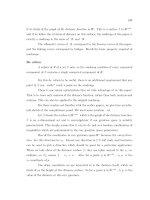
be measured by attaching a Hall Effect sensor at the top of the ball and manually moving
the ball up or down within the possible working range. One measurement is shown in

Fig. 6. By using the curve fitting technique, a 4th order polynominal is obtained as

(2)
with coefficients listed in Table. 1. In the following, equation (2) is used as the model of NIB
magnetic field.


Fig. 6. Measured magnetic field generated by NIB via distance

Table.1. Coefficients of B
b
(x) induced by NIB magnet
3.2 Nonlinear system model
Under assumption that the used material has a linear characteristic, i.e., the magnetization
density only depends on the magnetic field density (Woodson & Melcher (1968)), the
magnetic flux of the entire field, denoted as λ (t), can be approximated by

(3)
where i(t) denotes the current through the solenoid, and x (t) denotes the displacement of
the levitated object to the solenoid bottom. L(x) denotes the inductance when the levitated
object is assumed to be iron/steel and it can be regarded as a function of x (t) (Wong (1986);
Yang & Pedersen (2006)). λ
B
(x) is the flux introduced by the NIB magnet, and it also is a
Model-Based Control of a Nonlinear One Dimensional Magnetic Levitation with
a Permanent-Magnet Object

365
function of x(t) as we find out in eq.(2). By using the proposed approximation in (Wong
(1986); Oliveira et al. (1999); Yang & Pedersen (2006)), L(x) can be expressed as


(4)
where L
0
= L(0) - L(∞), L
1
= L(∞) and a is a constant coefficient.
According to the electromagnetic theory (Woodson & Melcher (1968)), the magnetic co-
energy, denoted as W, can be calculated as

(5)
By inserting (3) and (4) into (5), there is

(6)
The introduced magnetic force, denoted as f(t), is determined from the magnetic co-energy
according to

where x
a
represents the force acting axis, which is equal to the x(t) axis. Then from (6) we
have

(7)
Assume that the magnetic flux λ
B
(x) and the magnetic flux density have a constant linear
relationship. It could be reasonable if the considered system only has small moving distance.
There is

(8)

where B
b
(x) is the value calculated from equation (2). Therefore,
()
B
d
d
x
x
λ
can be
approximated by

(9)
Automation and Robotics

366
with coefficients given in Table 1.
Denote the mass of the levitating object as m and the gravity acceleration as g. By neglecting
the air drag friction, the dynamic of the levitating object can be obtained from Newton's
Second Law as

By inserting (7) into the above equation, there is

(10)
Compared with models used in (Barie & Chiasson (1996); Oliveira et al. (1999); Pedersen &
Yang (2006); Wong (1986); Yang & Pedersen (2006)), the third term on the right side of
equation (10) is new and it is due to the existing of the permanent NIB magnet.
Through circuit analysis, the electrical perspective of the solenoid can be modeled as


(11)
where R is the coil resistance, and u(t) is the input voltage to the coil. Compared with
models used in (Barie & Chiasson (1996); Oliveira et al. (1999); Pedersen & Yang (2006);
Wong (1986); Yang & Pedersen (2006)), the second term on the right side of (11) is new, and
it is the EMF induced by the permanent NIB magnet.
By taking relationship (8) and substituting (4) and (2) into (11), there is


(12)
Without triviality, if a small operating range is considered, the inductance (4) can be
approximated by a constant value (L = 0.1398H). In addition, by taking the linear part of
λ
B
(x), a linear version of equation (12) can be derived as

(13)
which is similar to a simplified linear DC-motor model (Woodson & Melcher (1968)).
Equations (10) and (12) constitute of a nonlinear model of the considered levitation system.
Model-Based Control of a Nonlinear One Dimensional Magnetic Levitation with
a Permanent-Magnet Object

367
Compared with models used in (Barie & Chiasson (1996); Oliveira et al. (1999); Pedersen &
Yang (2006); Wong (1986); Yang & Pedersen (2006)), here the influence of the NIB magnet is
reflected by the extra force in (10) and the EMF part in (12), respectively.
3.3 Coefficient identification
System coefficients L
0
, L(0) and L
1

used in (4) can be directly measured or estimated.
However, coefficients a and β
B
in (10) need to be identified through an experimental
approach similar to those used in (Oliveira et al. (1999); Yang & Pedersen (2006)). A set of
experiments is organized to find the currents required to levitate the object at different
equilibrium positions. The result is plotted in Fig. 7.


Fig. 7. The equilibrium points and corresponding required currents
By picking up three close equilibrium points and their corresponding currents, denoted as
x
1
, x
2
,x
3
and i
1
, i
2
, i
3
, respectively, from (7) there is

and

Coefficient a can be calculated by combining the above two equations. After a is determined,
β
B

can be determined based on any set, e.g., set (x
1
, i
1
). A simple way to determine a is to
assume the term β
B
B
b
(x
k
) i
k
is almost constant for k = 1, 2, 3. This assumption is reasonable
for a small operating range, so a can be determined by

(14)
Correspondingly, β
B
can be determined by