AUTOMATION&CONTROL-TheoryandPractice316

(4) component_X_bad_quality IF crumbs_in_material
These rules constitute only a small section of a diagnosis knowledge base for a real world
application. The causes of symptoms are situated on the left side of the IF statement, while
the symptoms itself are positioned on the right side. This is in opposite direction of the
causal direction. The results of the application of the reasoning algorithms are the
conclusions of the rules on the left-hand side of the IF statement and the result should be by
definition the cause of symptoms.
The syntax of the propositional logic has been defined in various books like (Kreuzer and
Kühling, 2006), (Russel and Norvig, 2003) or (Poole et al., 1998). Propositional formulae deal
only with the truth values {TRUE, FALSE} and a small set of operations is defined including
negation, conjunction, disjunction, implication and bi-conditional relations. The possibility
to nest formulae enables arbitrary large formulae.
The HLD restricts the propositional logic to Horn-logic, which is not a big limitation. A
Horn formula is a propositional formula in conjunctive normal form (a conjunction of
disjunctions) in which each disjunction contains in maximum one positive literal. The set of
elements of these disjunctions is also called a Horn clause. A set of Horn clauses build a
logic program. If a Horn clause contains exactly one positive and at least one negative
literal, then it is called a rule. The positive literal is the conclusion (or head) of the rule, while
the negative literals constitute the condition part (or the body) of the rule. If a rule is part of
a HLD file, then we call it a HLD rule.
The form of horn clauses is chosen for the HLD, since there exist an efficient reasoning
algorithm for this kind of logic - namely the SLD resolution. This resolution algorithm may
be combined with the breadth-first search (BFS) or with the depth-first search (DFS)
strategy.
 Breadth-first search: The algorithm proves for each rule whether the conclusion is a
consequence of the values of the conditions. Each condition value is either looked up in a
variable value mapping table or it will be determined by consideration of rules, which
have the same literal as conclusion. If there exist such rules, but a direct evaluation of
their conclusion is not possible, then a reference to this rule is stored, but the algorithm

proceeds with the next condition of the original rule. If there is no condition left in the
original rule, then references are restored and the same algorithm as for the original rule
is applied to the referenced rules. This approach needs a huge amount of memory.
 Depth-first search: This algorithm proves for each rule whether the conclusion is a
consequence of the values of the conditions. Each condition value is looked up in a
variable value mapping table or it will be determined by consideration of rules, which
have the same literal as conclusion. If there exist such rules, but a direct evaluation of the
conclusion is not possible then the first of these rules is evaluated directly. Therefore this
algorithm does not need the references and saves a lot of memory compared to BFS.
It may be shown that the SLD resolution with BFS strategy is complete for Horn logic while
the combination with DFS is incomplete. However, DFS is much more memory efficient
than BFS and in practise it leads often very quickly to the result values. Thus both resolution
algorithms have been prototypically implemented for evaluation of HLD files. The syntax of
the HLD does not depend on the selection of search algorithms.
The propositional variables of HLD rules have special meanings for the diagnosis purposes.
Following has been defined:

 Symptoms are propositional variables, which appear only as conditions within HLD
rules.
 Indirect failure causes are propositional variables, which appear as conclusion in some
HLD rules and in other HLD rules condition part.
 Direct failure causes are propositional variables, which appear only as conclusions of
HLD rules.
Thus simple propositional logic is modelled in the HLD by direct and indirect failure causes
as conclusion of rules and by symptoms and indirect failure causes as conditions of rules.

3.2.2 HLD Rules with Empirical Uncertainty Factors
The application of HLD rules is not always applicable or at least not very comfortable
because of the following reasons:
 A huge amount of rules and symptoms have to be defined in order to find failure causes

in complex technical systems. This is accompanied by very large condition parts of the
rules. The establishment of the knowledge base becomes too expensive.
 A diagnosis expert system, which has a high complex knowledge base, has to ask the
users for a lot of symptoms in order to find a failure cause. Guided diagnosis becomes
too time-consuming.
 Complex knowledge bases lead to long-term reasoning.
All these effects should be avoided according to the defined requirements. The mapping of
simple cause-effect relations with simple HLD rules continues to be applicable. But complex
circumstances need other kinds of expressivity.
A simple extension of HLD rules is the introduction of certainty factors (CF). Therein the
conclusion of a rule is weighted with a certainty factor. Such systems are described for
example in (Bratko, 2000), (Norvig, 1992) and (Janson, 1989). In these resources the value
range for the certainty factors is the interval [-1, +1]. For a better comparability of the CFs
with probabilities the interval [0, 1] has been chosen for certainty factors of HLD rules.
All propositions, which are evaluated by application of an algorithm on a HLD knowledge
base, are weighted by a CF, since the conclusion parts of the rules are weighted by certainty
factors. Certainty factors of propositions have the following semantic within HLD files:
CF = 0.0 The proposition is false.
CF = 0.5 It is unknown if the proposition is true or false.
CF = 1.0 The proposition is true.
CF values between 0.5 and 1.0 have the meaning that the related propositions are more
likely true than false, while CF values between 0.5 and 0.0 mean, that the related
propositions are more likely false than true.
Two algorithms for the evaluation of HLD rules with certainty factors have been tested.
These are the simple evaluation algorithm according to (Janson, 1989) and the EMYCIN
algorithm as shown in (Norvig, 1992). The simple algorithm is based on the following
instructions:
1. The CF of the condition part of a rule is the minimum CF of all the conditions.
2. The CF of the conclusion of a rule is the CF of the condition part of this rule multiplied
with the CF value for this rule.

3. If the knowledge base contains multiple rules with the same conclusion, then the CF of
this conclusion is the maximum of the related CF values.
ModularandHybridExpertSystemforPlantAssetManagement 317

(4) component_X_bad_quality IF crumbs_in_material
These rules constitute only a small section of a diagnosis knowledge base for a real world
application. The causes of symptoms are situated on the left side of the IF statement, while
the symptoms itself are positioned on the right side. This is in opposite direction of the
causal direction. The results of the application of the reasoning algorithms are the
conclusions of the rules on the left-hand side of the IF statement and the result should be by
definition the cause of symptoms.
The syntax of the propositional logic has been defined in various books like (Kreuzer and
Kühling, 2006), (Russel and Norvig, 2003) or (Poole et al., 1998). Propositional formulae deal
only with the truth values {TRUE, FALSE} and a small set of operations is defined including
negation, conjunction, disjunction, implication and bi-conditional relations. The possibility
to nest formulae enables arbitrary large formulae.
The HLD restricts the propositional logic to Horn-logic, which is not a big limitation. A
Horn formula is a propositional formula in conjunctive normal form (a conjunction of
disjunctions) in which each disjunction contains in maximum one positive literal. The set of
elements of these disjunctions is also called a Horn clause. A set of Horn clauses build a
logic program. If a Horn clause contains exactly one positive and at least one negative
literal, then it is called a rule. The positive literal is the conclusion (or head) of the rule, while
the negative literals constitute the condition part (or the body) of the rule. If a rule is part of
a HLD file, then we call it a HLD rule.
The form of horn clauses is chosen for the HLD, since there exist an efficient reasoning
algorithm for this kind of logic - namely the SLD resolution. This resolution algorithm may
be combined with the breadth-first search (BFS) or with the depth-first search (DFS)
strategy.
 Breadth-first search: The algorithm proves for each rule whether the conclusion is a
consequence of the values of the conditions. Each condition value is either looked up in a

variable value mapping table or it will be determined by consideration of rules, which
have the same literal as conclusion. If there exist such rules, but a direct evaluation of
their conclusion is not possible, then a reference to this rule is stored, but the algorithm
proceeds with the next condition of the original rule. If there is no condition left in the
original rule, then references are restored and the same algorithm as for the original rule
is applied to the referenced rules. This approach needs a huge amount of memory.
 Depth-first search: This algorithm proves for each rule whether the conclusion is a
consequence of the values of the conditions. Each condition value is looked up in a
variable value mapping table or it will be determined by consideration of rules, which
have the same literal as conclusion. If there exist such rules, but a direct evaluation of the
conclusion is not possible then the first of these rules is evaluated directly. Therefore this
algorithm does not need the references and saves a lot of memory compared to BFS.
It may be shown that the SLD resolution with BFS strategy is complete for Horn logic while
the combination with DFS is incomplete. However, DFS is much more memory efficient
than BFS and in practise it leads often very quickly to the result values. Thus both resolution
algorithms have been prototypically implemented for evaluation of HLD files. The syntax of
the HLD does not depend on the selection of search algorithms.
The propositional variables of HLD rules have special meanings for the diagnosis purposes.
Following has been defined:

 Symptoms are propositional variables, which appear only as conditions within HLD
rules.
 Indirect failure causes are propositional variables, which appear as conclusion in some
HLD rules and in other HLD rules condition part.
 Direct failure causes are propositional variables, which appear only as conclusions of
HLD rules.
Thus simple propositional logic is modelled in the HLD by direct and indirect failure causes
as conclusion of rules and by symptoms and indirect failure causes as conditions of rules.

3.2.2 HLD Rules with Empirical Uncertainty Factors

The application of HLD rules is not always applicable or at least not very comfortable
because of the following reasons:
 A huge amount of rules and symptoms have to be defined in order to find failure causes
in complex technical systems. This is accompanied by very large condition parts of the
rules. The establishment of the knowledge base becomes too expensive.
 A diagnosis expert system, which has a high complex knowledge base, has to ask the
users for a lot of symptoms in order to find a failure cause. Guided diagnosis becomes
too time-consuming.
 Complex knowledge bases lead to long-term reasoning.
All these effects should be avoided according to the defined requirements. The mapping of
simple cause-effect relations with simple HLD rules continues to be applicable. But complex
circumstances need other kinds of expressivity.
A simple extension of HLD rules is the introduction of certainty factors (CF). Therein the
conclusion of a rule is weighted with a certainty factor. Such systems are described for
example in (Bratko, 2000), (Norvig, 1992) and (Janson, 1989). In these resources the value
range for the certainty factors is the interval [-1, +1]. For a better comparability of the CFs
with probabilities the interval [0, 1] has been chosen for certainty factors of HLD rules.
All propositions, which are evaluated by application of an algorithm on a HLD knowledge
base, are weighted by a CF, since the conclusion parts of the rules are weighted by certainty
factors. Certainty factors of propositions have the following semantic within HLD files:
CF = 0.0 The proposition is false.
CF = 0.5 It is unknown if the proposition is true or false.
CF = 1.0 The proposition is true.
CF values between 0.5 and 1.0 have the meaning that the related propositions are more
likely true than false, while CF values between 0.5 and 0.0 mean, that the related
propositions are more likely false than true.
Two algorithms for the evaluation of HLD rules with certainty factors have been tested.
These are the simple evaluation algorithm according to (Janson, 1989) and the EMYCIN
algorithm as shown in (Norvig, 1992). The simple algorithm is based on the following
instructions:

1. The CF of the condition part of a rule is the minimum CF of all the conditions.
2. The CF of the conclusion of a rule is the CF of the condition part of this rule multiplied
with the CF value for this rule.
3. If the knowledge base contains multiple rules with the same conclusion, then the CF of
this conclusion is the maximum of the related CF values.
AUTOMATION&CONTROL-TheoryandPractice318

The algorithms for certainty factors are proved to provide incorrect results in some
situations. On the other hand for MYCIN it has been shown that such systems may provide
better results than human experts. In addition the rule CFs may be empirically determined
and thus the creation of a knowledge base is very easy. For these reasons the concept of
certainty factors has been included into the HLD language.

3.2.3 Fuzzy Logic as Part of the HLD
Rule sets as described in the previous sections use mappings of diagnosis relevant physical
values to discrete values as propositions. Thus rules for each discrete value interval have to
be provided. This leads to a big effort for the creation of the knowledge base. In this section
we introduce Fuzzy Logic as one opportunity to improve the preciseness of the reasoning
and to reduce the necessity for fine grained discretization levels of physical values. An
example of a HLD fuzzy logic rule is the following:
motor_defect WITH 0.9 IF motor_windings_hot AND load_low.
The way of diagnosis is different from that of the propositional logic. The diagnosis user
inputs values of continuous value spaces (in the example for motor winding temperature
and mechanical load), instead of providing discrete symptoms and binary answering of
questions. The result is again a value out of a continuous value space (in the example an
estimation of the degree of abrasion of the motor). Special diagnosis relevant output
variables have been defined for the HLD language.
The use of Fuzzy Logic for diagnosis purposes works in following steps:
1. Definition of the knowledge base: (A) Fuzzy variables have to be defined and (B) a
Fuzzy rule set has to be integrated into the knowledge base.

2. Evaluation of the knowledge base: (C) The user inputs variable values and (D) the
implementation of a Fuzzy Logic interpreter provides results by fuzzyfication of input
variables, applying of inferences and by defuzzyfication of output variables.
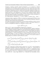
Fuzzy variables may be defined by mapping of triangles, trapezoids or more round function
shapes to terms of natural language. Input variables within the HLD fuzzy logic may be
defined by piecewise linear membership functions, while output variables are defined by
singletons (see figure 2).

Fuzzy input variable „A“
(a single piecewise linear
linguistic term)
Fuzzy output variable „B“
(singletons)
1.0
0.5
0.0
μ
A
(x)
x
x
1
x
2
x
3
x
4
x
5

μ
A 1,5
μ
A 2
μ
A 3,4
1.0
0.5
0.0
μ
B
(y)
y
y
1
y
2
y
3
μ
B 1,2,3

Fig. 2. HLD Fuzzy Logic input and output variables

This definition is in line with the standard (IEC61131-7, 1997). This is the standard for
programming languages for programmable logic controllers (PLC). PLCs are the most used
automation systems for machinery and plant control. Thus if the maintenance employees
know something about Fuzzy Logic then it is very likely, that they know the terminology
and semantics of this standard.


Maintenance-Fuzzy-Variable „IH“
(Singletons in range: 0 ≤ y
IH i
≤ 1)
1.0
0.5
0.0
μ(y
IH
)
y
IH
y
IH 1
y
IH 2
y
IH n-1
y
IH n
. . .
1.0
. . .
0.0
maintenance required
or failure cause
none maintenance required
or no failure cause

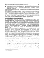
Fig. 3. HLD maintenance fuzzy variables


Beside the common semantics of Fuzzy output variables there are special definitions for
maintenance variables in the HLD specification. This is illustrated in figure 3. The values of
such variables y
IH
are defined only within a range of [0, 1.0]. Only within this value range
singletons may be defined. Similar to the definitions for certainty factors following
conventions have been defined for these maintenance variables:
y
IH
= 0.0 Maintenance is not necessary or this is not a failure cause.
y
IH
= 0.5 It is not decidable if this is a failure cause.
y
IH
= 1.0 Maintenance is necessary since this is a failure cause.
As mentioned above the processing of the maintenance knowledge base is done in three
steps:
1. Fuzzyfication: Memberships are computed for each linguistic term of the input
variables if there are numerical values available for the physical input variables.
2. Inference: The inference is done very similar to the approach used for rule sets with
certainty factors:
a. The membership of the condition part of a fuzzy rule is the minimum of
all the memberships of the condition variables.
b. The membership of the conclusion of a fuzzy rule is the membership of
the condition part of this rule multiplied with the weighting factor for this
rule.
c. If the knowledge base contains multiple fuzzy rules with the same
conclusion, then the membership of this conclusion is the maximum of the

membership values of the conclusion variables.
ModularandHybridExpertSystemforPlantAssetManagement 319

The algorithms for certainty factors are proved to provide incorrect results in some
situations. On the other hand for MYCIN it has been shown that such systems may provide
better results than human experts. In addition the rule CFs may be empirically determined
and thus the creation of a knowledge base is very easy. For these reasons the concept of
certainty factors has been included into the HLD language.

3.2.3 Fuzzy Logic as Part of the HLD
Rule sets as described in the previous sections use mappings of diagnosis relevant physical
values to discrete values as propositions. Thus rules for each discrete value interval have to
be provided. This leads to a big effort for the creation of the knowledge base. In this section
we introduce Fuzzy Logic as one opportunity to improve the preciseness of the reasoning
and to reduce the necessity for fine grained discretization levels of physical values. An
example of a HLD fuzzy logic rule is the following:
motor_defect WITH 0.9 IF motor_windings_hot AND load_low.
The way of diagnosis is different from that of the propositional logic. The diagnosis user
inputs values of continuous value spaces (in the example for motor winding temperature
and mechanical load), instead of providing discrete symptoms and binary answering of
questions. The result is again a value out of a continuous value space (in the example an
estimation of the degree of abrasion of the motor). Special diagnosis relevant output
variables have been defined for the HLD language.
The use of Fuzzy Logic for diagnosis purposes works in following steps:
1. Definition of the knowledge base: (A) Fuzzy variables have to be defined and (B) a
Fuzzy rule set has to be integrated into the knowledge base.
2. Evaluation of the knowledge base: (C) The user inputs variable values and (D) the
implementation of a Fuzzy Logic interpreter provides results by fuzzyfication of input
variables, applying of inferences and by defuzzyfication of output variables.
Fuzzy variables may be defined by mapping of triangles, trapezoids or more round function

shapes to terms of natural language. Input variables within the HLD fuzzy logic may be
defined by piecewise linear membership functions, while output variables are defined by
singletons (see figure 2).

Fuzzy input variable „A“
(a single piecewise linear
linguistic term)
Fuzzy output variable „B“
(singletons)
1.0
0.5
0.0
μ
A
(x)
xx
1
x
2
x
3
x
4
x
5
μ
A 1,5
μ
A 2
μ

A 3,4
1.0
0.5
0.0
μ
B
(y)
yy
1
y
2
y
3
μ
B 1,2,3

Fig. 2. HLD Fuzzy Logic input and output variables

This definition is in line with the standard (IEC61131-7, 1997). This is the standard for
programming languages for programmable logic controllers (PLC). PLCs are the most used
automation systems for machinery and plant control. Thus if the maintenance employees
know something about Fuzzy Logic then it is very likely, that they know the terminology
and semantics of this standard.

Maintenance-Fuzzy-Variable „IH“
(Singletons in range: 0 ≤ y
IH i
≤ 1)
1.0
0.5

0.0
μ(y
IH
)
y
IH
y
IH 1
y
IH 2
y
IH n-1
y
IH n
. . .
1.0
. . .
0.0
maintenance required
or failure cause
none maintenance required
or no failure cause

Fig. 3. HLD maintenance fuzzy variables

Beside the common semantics of Fuzzy output variables there are special definitions for
maintenance variables in the HLD specification. This is illustrated in figure 3. The values of
such variables y
IH
are defined only within a range of [0, 1.0]. Only within this value range

singletons may be defined. Similar to the definitions for certainty factors following
conventions have been defined for these maintenance variables:
y
IH
= 0.0 Maintenance is not necessary or this is not a failure cause.
y
IH
= 0.5 It is not decidable if this is a failure cause.
y
IH
= 1.0 Maintenance is necessary since this is a failure cause.
As mentioned above the processing of the maintenance knowledge base is done in three
steps:
1. Fuzzyfication: Memberships are computed for each linguistic term of the input
variables if there are numerical values available for the physical input variables.
2. Inference: The inference is done very similar to the approach used for rule sets with
certainty factors:
a. The membership of the condition part of a fuzzy rule is the minimum of
all the memberships of the condition variables.
b. The membership of the conclusion of a fuzzy rule is the membership of
the condition part of this rule multiplied with the weighting factor for this
rule.
c. If the knowledge base contains multiple fuzzy rules with the same
conclusion, then the membership of this conclusion is the maximum of the
membership values of the conclusion variables.
AUTOMATION&CONTROL-TheoryandPractice320

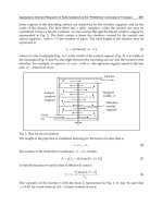
3. Defuzzyfication: Within the basic level of conformance of the standard (IEC61131-7,
1997) the method "Center of Gravity for Singletons" (COGS) has been defined as
defuzzyfication method. This has been taken over for the HLD specification. The result

value of the fuzzy logic output variable is computed by evaluation of following
formula:





p
i
Bi
p
i
i
Bi
y
y
1
*
1
*
)(



This formula uses the terminology as presented in figure 2. The
μ*
Bi
are the
membership values computed in the inference process for the p singletons at the values
y

i
. The result value y is the value of the output variable. Thus it is not a membership
but a value of the value range defined for this output variable. Especially for the
maintenance output variables the value range is [0, 1].
The approach of using singletons fits the need of fast computations as specified in the
requirements analysis, since only multiplication and addition operations are used.

3.2.4 Bayesian Networks
Bayesian Networks have been introduced into the HLD, since the handling of uncertainty
with certainty factors is not as mathematically correct as the probability theory does.
The example introduced in the propositional logic section could be extended by
probabilities as follows
component_X_bad_quality (p=0.9) IF crumbs_in_material.
component_X_bad_quality (p=0.5) IF product_color_grey.
This example has the meaning that if there are crumbs in the raw material then the
probability are very high (90%) that the material component X has not a good quality. In
other words there are not many other reasons for crumbs than a bad material X. But there is
another phenomenon in that approach: the variables crumbs_in_material and
product_color_grey are not independent from each other. If there are crumbs in the
material, then it is likely that the component X has a bad quality, but then there is also a
good chance that the product looks a little bit grey.
Bayesian Networks are graphical representations (directed acyclic graphs) of such rules as
shown in the example. (Ertel, 2008) gives a good introduction to Bayesian Networks based
on (Jensen, 2001). One of the earlier literature references is (Pearl, 1988). There are following
principles of reasoning in Bayesian Networks:
 Naive computations of Bayesian Networks. This algorithm computes the probabilities
for every node of the network. The computation is simple but very inefficient. (Bratko,
2000) presents an implementation of this algorithm for illustration of the principles.
 Clustering algorithms for Bayesian Networks. This approach uses special properties of
Bayesian Networks (d-Separation) for dividing the network into smaller pieces

(clusters). Each of the clusters may be separately computed. For each cluster it is decided
if it is influenced by evident variables. The computation of probabilities is done only for
these clusters. The approach is much more efficient than the naive approach.

 Approximation of Bayesian Networks. Algorithms of this concept estimate the
probability of variables. Such algorithms may be used even in cases where clustering
algorithms need too much time.
The naive algorithm has been implemented for the evaluation of the usability of Bayesian
Networks for the HLD. Further evaluation has been done by using the SMILE reasoning
engine for graphical probabilistic models contributed by the Decision Systems Laboratory of
the University Pittsburgh ().

3.2.5 Summary and the HLD Language Schema
XML has been chosen as basic format of the HLD. Thus an XML schema according to W3C
standards has been developed, which contains language constructs for the methodologies
described in the previous sections. The structure of this schema is shown in figure 4.


Fig. 4. HLD schema overview.

The HLD schema contains following top level information:
 Meta Information. The element MetaInf contains various common information about the
asset described by the HLD file. This includes for example the manufacturer name, an
ordering number, a short description and a service URL for getting further information
from the manufacturer.
ModularandHybridExpertSystemforPlantAssetManagement 321

3. Defuzzyfication: Within the basic level of conformance of the standard (IEC61131-7,
1997) the method "Center of Gravity for Singletons" (COGS) has been defined as
defuzzyfication method. This has been taken over for the HLD specification. The result

value of the fuzzy logic output variable is computed by evaluation of following
formula:





p
i
Bi
p
i
i
Bi
y
y
1
*
1
*
)(



This formula uses the terminology as presented in figure 2. The
μ*
Bi
are the
membership values computed in the inference process for the p singletons at the values
y

i
. The result value y is the value of the output variable. Thus it is not a membership
but a value of the value range defined for this output variable. Especially for the
maintenance output variables the value range is [0, 1].
The approach of using singletons fits the need of fast computations as specified in the
requirements analysis, since only multiplication and addition operations are used.

3.2.4 Bayesian Networks
Bayesian Networks have been introduced into the HLD, since the handling of uncertainty
with certainty factors is not as mathematically correct as the probability theory does.
The example introduced in the propositional logic section could be extended by
probabilities as follows
component_X_bad_quality (p=0.9) IF crumbs_in_material.
component_X_bad_quality (p=0.5) IF product_color_grey.
This example has the meaning that if there are crumbs in the raw material then the
probability are very high (90%) that the material component X has not a good quality. In
other words there are not many other reasons for crumbs than a bad material X. But there is
another phenomenon in that approach: the variables crumbs_in_material and
product_color_grey are not independent from each other. If there are crumbs in the
material, then it is likely that the component X has a bad quality, but then there is also a
good chance that the product looks a little bit grey.
Bayesian Networks are graphical representations (directed acyclic graphs) of such rules as
shown in the example. (Ertel, 2008) gives a good introduction to Bayesian Networks based
on (Jensen, 2001). One of the earlier literature references is (Pearl, 1988). There are following
principles of reasoning in Bayesian Networks:
 Naive computations of Bayesian Networks. This algorithm computes the probabilities
for every node of the network. The computation is simple but very inefficient. (Bratko,
2000) presents an implementation of this algorithm for illustration of the principles.
 Clustering algorithms for Bayesian Networks. This approach uses special properties of
Bayesian Networks (d-Separation) for dividing the network into smaller pieces

(clusters). Each of the clusters may be separately computed. For each cluster it is decided
if it is influenced by evident variables. The computation of probabilities is done only for
these clusters. The approach is much more efficient than the naive approach.

 Approximation of Bayesian Networks. Algorithms of this concept estimate the
probability of variables. Such algorithms may be used even in cases where clustering
algorithms need too much time.
The naive algorithm has been implemented for the evaluation of the usability of Bayesian
Networks for the HLD. Further evaluation has been done by using the SMILE reasoning
engine for graphical probabilistic models contributed by the Decision Systems Laboratory of
the University Pittsburgh ().

3.2.5 Summary and the HLD Language Schema
XML has been chosen as basic format of the HLD. Thus an XML schema according to W3C
standards has been developed, which contains language constructs for the methodologies
described in the previous sections. The structure of this schema is shown in figure 4.


Fig. 4. HLD schema overview.

The HLD schema contains following top level information:
 Meta Information. The element MetaInf contains various common information about the
asset described by the HLD file. This includes for example the manufacturer name, an
ordering number, a short description and a service URL for getting further information
from the manufacturer.
AUTOMATION&CONTROL-TheoryandPractice322

 Variable Declarations. The element VariableList contains lists of variables. Propositional
variables (with and without certainty factors) are separated from Fuzzy Logic input and
output variables due to their different representation models.

 Knowledge Base. This element contains the following sub elements:
o Logic: This element contains rules with and without the use of certainty factors.
o Fuzzy Logic: This element contains fuzzy logic rules and it references the Fuzzy
Logic input and output variables.
o Bayesian Network: This element contains the definition of a Bayesian Network for
discrete variables. It contains conditional probability tables and references to the
declarations of propositional variables.
The other attributes and elements define the semantics as specified in the sections above.
The full HLD scheme may be downloaded at "

4. Framework for the Handling of the Knowledge Base

The central application of the HLD framework is the diagnosis system. It is implemented as
a web application. This provides the possibilities to:
 maintain the knowledge base on one place,
 enable the access to the diagnosis system from any place,
 reduce the necessity of installation of special software (a Web browser is expected to be
installed on any modern operating system by default).


Fig. 5. HLD interpreter as web application


Figure 5 gives an overview of this application. On the left side the expert system provides a
list of possible symptoms. The diagnosis user marks, which symptoms he has percepted.
The diagnosis results are listed on the right side, sorted by their probability or their
membership to a maintenance fuzzy variable.
The expert has another application for the creation of the knowledge for a specific asset
type. This is an editor for HLD files. A screenshot of a prototype application is shown in
figure 6. On the left side there is a tree representing the asset hierarchy. Elements of this tree

are set into relations by definition of rules. This is done by entering some input into the
forms of the right side. The screenshot shows the forms for input of logic rules. The entry
fields are labelled by using the maintenance terminology. Thus a transformation of the
terminology of artificial intelligence terminology to the application domain is done by this
user frontend for the asset experts. The HLD editor uses for example the term "failure cause"
('Schadensursache') instead of the term "conclusion" or "clause head".


Fig. 6. HLD editor.

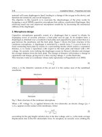
Assets like machine and plants are recursively nested when considering the aggregation
relation. This is illustrated in fig. 7. If we consider a plant as asset, then the machines are the
asset elements. If we further consider the machines as assets, then the tools, HMI elements
and the control system are the asset elements. The HLD language introduces elements with
the name "Context" in order to reference aggregated asset elements (see also fig. 4).

ModularandHybridExpertSystemforPlantAssetManagement 323

 Variable Declarations. The element VariableList contains lists of variables. Propositional
variables (with and without certainty factors) are separated from Fuzzy Logic input and
output variables due to their different representation models.
 Knowledge Base. This element contains the following sub elements:
o Logic: This element contains rules with and without the use of certainty factors.
o Fuzzy Logic: This element contains fuzzy logic rules and it references the Fuzzy
Logic input and output variables.
o Bayesian Network: This element contains the definition of a Bayesian Network for
discrete variables. It contains conditional probability tables and references to the
declarations of propositional variables.
The other attributes and elements define the semantics as specified in the sections above.
The full HLD scheme may be downloaded at "


4. Framework for the Handling of the Knowledge Base

The central application of the HLD framework is the diagnosis system. It is implemented as
a web application. This provides the possibilities to:
 maintain the knowledge base on one place,
 enable the access to the diagnosis system from any place,
 reduce the necessity of installation of special software (a Web browser is expected to be
installed on any modern operating system by default).


Fig. 5. HLD interpreter as web application


Figure 5 gives an overview of this application. On the left side the expert system provides a
list of possible symptoms. The diagnosis user marks, which symptoms he has percepted.
The diagnosis results are listed on the right side, sorted by their probability or their
membership to a maintenance fuzzy variable.
The expert has another application for the creation of the knowledge for a specific asset
type. This is an editor for HLD files. A screenshot of a prototype application is shown in
figure 6. On the left side there is a tree representing the asset hierarchy. Elements of this tree
are set into relations by definition of rules. This is done by entering some input into the
forms of the right side. The screenshot shows the forms for input of logic rules. The entry
fields are labelled by using the maintenance terminology. Thus a transformation of the
terminology of artificial intelligence terminology to the application domain is done by this
user frontend for the asset experts. The HLD editor uses for example the term "failure cause"
('Schadensursache') instead of the term "conclusion" or "clause head".


Fig. 6. HLD editor.


Assets like machine and plants are recursively nested when considering the aggregation
relation. This is illustrated in fig. 7. If we consider a plant as asset, then the machines are the
asset elements. If we further consider the machines as assets, then the tools, HMI elements
and the control system are the asset elements. The HLD language introduces elements with
the name "Context" in order to reference aggregated asset elements (see also fig. 4).

AUTOMATION&CONTROL-TheoryandPractice324

Asset-
element
(x)
Asset-
element
(x+1)
Asset-
element
(x+n)
. . .
Failure cause
Failure symptom
Asset context

Fig. 7. Failure cause and symptom relation within an asset

In many cases failures occur in one asset element and cause symptoms in another asset
element. These relations may be described in HLD files dedicated to the upper asset context,
which contains the related asset elements directly or indirectly.
All HLD descriptions of the assets and their recursively nested aggregates build the
knowledge base of the diagnosis expert system. They are positioned side by side in a HLD

file repository. Each HLD description is dedicated to an asset type and its version, which are
represented by structure elements of the repository. Thus the repository is not free form. It is
obviously from fig. 7, that an asset description must be the assembly of the asset context
description and the descriptions of all asset elements. Thus a HLD description is a package
of HLD files with the same structure like a HLD repository. The tool set contains a
packaging system, which assembles all necessary HLD descriptions from the repository of
the asset expert and compresses them. Furthermore the tool set contains a package
installation system, which decompresses the packages and installs them in a HLD
repository, while paying attention to asset type and version information. In addition a
documentation generation system has been set up, which generates HTML files out of a
repository by a given asset context.

5. Conclusions and Future Research Work

An expert system has been introduced with a hybrid knowledge base in that sense that it
uses multiple paradigms of the artificial intelligence research work. There was a gap
between the success of the theoretical work and the acceptance in the industry. One key
problem is the necessary effort for the creation of the knowledge base, which is overcome by
the concept of a collaborative construction of the knowledge base by contributions of
manufacturers of the production equipment.
Further research work will be spent to structure and parameter learning algorithms for the
Bayesian Networks. The results have to be integrated into the HLD editor. Furthermore an
on-line data acquisition will be integrated into the diagnosis system, which is especially
necessary for an effective application of the Fuzzy Logic reasoning.
Most of the work has been done as part of the research project WISA. This project work has
been funded by the German Ministry of Economy and Employment. It is registered under
reg no. IW06215. The authors gratefully thank for this support by the German government.


6. References


Bratko, Ivan (2000). PROLOG - Programming for Artificial Intelligence, 3.Ed., Addison-
Wesley
Bronstein, Semendjajew, Musiol, Mühlig (1997). Taschenbuch der Mathematik, 3. Ed.,
Verlag Harri Deutsch
Ertel, W. (2008). Grundkurs künstliche Intelligenz, 1. Ed., Vieweg Verlag
IEC61131-7 (1997). IEC 61131 - Programmable Logic Controllers, Part 7 - Fuzzy Control
Programming, Committee Draft 1.0, International Electrotechnical Commission
(IEC)
Janson, Alexander (1989). Expertensysteme und Turbo-Prolog, 1. Ed., Franzis Verlag GmbH
München
Jensen, Finn V. (2001). Bayesian networks and decision graphs, Springer Verlag
Kreuzer, M.; Kühling, S. (2006). Logik für Informatiker, 1. Ed, Pearson Education
Deutschland GmbH
Norvig, Peter (1992). Paradigms of Artificial Intelligence Programming - Case Studies in
Lisp, 1. Ed., Morgan Kaufman Publishers, Inc.
Pearl, J. (1988). Probabilistic Reasoning in Intelligent Systems, Morgan Kaufmann
Publishers, Inc.
Poole, D.; Mackworth, A.; Goebel, R. (1998). Computational Intelligence - A Logical
Approach, 1. Ed., Oxford University Press, Inc.
Russell, S. and Norvig, P. (2003). Artificial Intelligence - A Modern Approach , 2. Ed.,
Pearson Education, Inc.

ModularandHybridExpertSystemforPlantAssetManagement 325

Asset-
element
(x)
Asset-
element

(x+1)
Asset-
element
(x+n)
. . .
Failure cause
Failure symptom
Asset context

Fig. 7. Failure cause and symptom relation within an asset

In many cases failures occur in one asset element and cause symptoms in another asset
element. These relations may be described in HLD files dedicated to the upper asset context,
which contains the related asset elements directly or indirectly.
All HLD descriptions of the assets and their recursively nested aggregates build the
knowledge base of the diagnosis expert system. They are positioned side by side in a HLD
file repository. Each HLD description is dedicated to an asset type and its version, which are
represented by structure elements of the repository. Thus the repository is not free form. It is
obviously from fig. 7, that an asset description must be the assembly of the asset context
description and the descriptions of all asset elements. Thus a HLD description is a package
of HLD files with the same structure like a HLD repository. The tool set contains a
packaging system, which assembles all necessary HLD descriptions from the repository of
the asset expert and compresses them. Furthermore the tool set contains a package
installation system, which decompresses the packages and installs them in a HLD
repository, while paying attention to asset type and version information. In addition a
documentation generation system has been set up, which generates HTML files out of a
repository by a given asset context.

5. Conclusions and Future Research Work


An expert system has been introduced with a hybrid knowledge base in that sense that it
uses multiple paradigms of the artificial intelligence research work. There was a gap
between the success of the theoretical work and the acceptance in the industry. One key
problem is the necessary effort for the creation of the knowledge base, which is overcome by
the concept of a collaborative construction of the knowledge base by contributions of
manufacturers of the production equipment.
Further research work will be spent to structure and parameter learning algorithms for the
Bayesian Networks. The results have to be integrated into the HLD editor. Furthermore an
on-line data acquisition will be integrated into the diagnosis system, which is especially
necessary for an effective application of the Fuzzy Logic reasoning.
Most of the work has been done as part of the research project WISA. This project work has
been funded by the German Ministry of Economy and Employment. It is registered under
reg no. IW06215. The authors gratefully thank for this support by the German government.


6. References

Bratko, Ivan (2000). PROLOG - Programming for Artificial Intelligence, 3.Ed., Addison-
Wesley
Bronstein, Semendjajew, Musiol, Mühlig (1997). Taschenbuch der Mathematik, 3. Ed.,
Verlag Harri Deutsch
Ertel, W. (2008). Grundkurs künstliche Intelligenz, 1. Ed., Vieweg Verlag
IEC61131-7 (1997). IEC 61131 - Programmable Logic Controllers, Part 7 - Fuzzy Control
Programming, Committee Draft 1.0, International Electrotechnical Commission
(IEC)
Janson, Alexander (1989). Expertensysteme und Turbo-Prolog, 1. Ed., Franzis Verlag GmbH
München
Jensen, Finn V. (2001). Bayesian networks and decision graphs, Springer Verlag
Kreuzer, M.; Kühling, S. (2006). Logik für Informatiker, 1. Ed, Pearson Education
Deutschland GmbH

Norvig, Peter (1992). Paradigms of Artificial Intelligence Programming - Case Studies in
Lisp, 1. Ed., Morgan Kaufman Publishers, Inc.
Pearl, J. (1988). Probabilistic Reasoning in Intelligent Systems, Morgan Kaufmann
Publishers, Inc.
Poole, D.; Mackworth, A.; Goebel, R. (1998). Computational Intelligence - A Logical
Approach, 1. Ed., Oxford University Press, Inc.
Russell, S. and Norvig, P. (2003). Artificial Intelligence - A Modern Approach , 2. Ed.,
Pearson Education, Inc.

AUTOMATION&CONTROL-TheoryandPractice326
ImageRetrievalSysteminHeterogeneousDatabase 327
ImageRetrievalSysteminHeterogeneousDatabase
KhalifaDjemal,HichemMaarefandRostomKachouri
X

Image Retrieval System in
Heterogeneous Database

Khalifa Djemal, Hichem Maaref and Rostom Kachouri
University of Evry Val d’Essonne, IBISC Laboratory
France

1. Introduction

This chapter content try to give readers theoretical and practical methods developed to
describes and recognize images in large database through different applications. Indeed,
many computer vision system applications, such as computer-human interaction,
controlling processes: autonomous vehicles, and industrial robots, have emerged a new
need for searching and browsing visual information. Furthermore, due to the fast
development of internet technologies, multimedia archives are growing rapidly, especially

digital image libraries which represent increasingly an important volume of information. So,
it is judicious to develop powerful browsing computer systems to handle, index, classify
and recognize images in these large databases. Different steps can be composes an image
retrieval system where the most important are, features extraction and classification.
Feature extraction and description of image content: Each feature is able to describe some
image characteristics related to shape, color or texture, but it cannot cover the entire visual
characteristics. Therefore, using multiple and different features to describe an image is
approved. In this chapter, the extraction of several features and description for
heterogeneous image database is presented and discussed. Test and choice of adequate
classifiers to manage correctly clustering and image recognition: The choice of the used
classifier in CBIR system (Content Based Image Retrieval) is very important. In this chapter
we present the Support vector machines (SVMs) as a supervised classification method
comprising mainly two stages: training and generalization. From these two important
points, we try how we can decide that the extracted features are relevant in large
heterogeneous database and the response to query image is acceptable. In these conditions
we must find compromise between precision of image recognition and computation time
which can be allowed to the CBIR System. In this aim, an heterogeneous image retrieval
system effectiveness is studied through a comparison between statistical and hierarchical
feature type models. The results are presented and discussed in relation with the used
images database, the selected features and classification techniques. The different sections of
this chapter recall and present the importance and the influence of the features relevance
and classification in image recognition and retrieval system. Indeed, different features
extraction methods (section 3) and classification approaches (section 4) are presented and
18
AUTOMATION&CONTROL-TheoryandPractice328

discussed. We illustrate the principle and obtained results of the optimization methods in
sections 5.

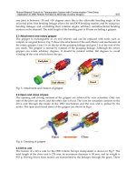
2. Related works


The image recognition system, consists of extracting from a Database all the similar images
to query images chosen by the user, figure 1, has attracted much research interest in recent
years. Principal difficulties consist on the capacity to extract from the image the visual
characteristics, the robustness to the geometrical deformations and the quantification of the
similarity concept between images. Indexation and recognition are given from a
classification methods accomplished on images features. To understand the influence of the
images database on the description method and the appropriate classification tool, it is more
convenient to subdivide the image databases into two categories.


Fig. 1. Content Based Image Recognition system.

The first category consists of image databases usually heterogeneous. In this context, the
objective of the images recognition system is to assist the user to intelligently search in
images database a particular subject adapting to the subjective needs of each user. The
second category concerns specific image databases. In this context, the images are most
often a uniform semantic content. The concerned applications are generally professional. To
index this image databases, the user must integrate more information defined by the expert
to develop a specific algorithm, the objective is to optimize system efficiency and its ability
to respond as well as the expert. This categorization is to be taken into account when
developing any content image retrieval system. Indeed, to obtain satisfactory results, the
choice or development of new description methods must be appropriate for the type of the
considered images database. This is due simply to the great difficulty to obtain a universal
description algorithm.
The content-based image retrieval that we have just described it in figure 1, have attracted
the attention of several specialists in different domains and caused for a few years an
important effort of research. Indeed, there has been growing interest in indexing large

biomedical images by content due to the advances in digital imaging and the increase

development of computer vision. Image recognition in biomedical databases, for example,
are critical assets for medical diagnosis. To facilitate automatic indexing and recognition of
image databases, several methods has been developed and proposed. As described above,
two important steps composed an image retrieval system, features extraction and
classification. We present in this section some important related work to these stages. We
find several choices of features from the low level to high level: shape, geometry, symbolic
features, .etc. The basic goal in content-based image retrieval and recognition is to bridge the
gap from the low-level image properties. Consequently, we can directly access to the objects,
and users generally want to find in image databases. For example, color histograms (Stricker
& Swain, 1994), (Swain & Ballard, 1991), are commonly used in image description and have
proven useful, however, this global characterization lacks information about how the color
is distributed spatially. Several researchers have attempted to overcome this limitation by
incorporating spatial information in the features extraction stage. Stricker and Dimai
(Stricker & Dimai, 1997), store the average color and the color covariance matrix within each
of five fuzzy image regions.
(Huang et al., 1997) store a color correlogram that encodes the spatial correlation of color-
bin pairs. (Smith & Chang, 1996), store the location of each color that is present in a
sufficient amount in regions computed using histogram back-projection. (Lipson et al., 1997)
retrieve images based on spatial and photometric relationships within and across simple
image regions. Little or no segmentation is done; the regions are derived from low-
resolution images. In (Jacobs et al., 1995), authors use multiresolution wavelet
decompositions to perform queries based on iconic matching. Some of these systems encode
information about the spatial distribution of color features, and some perform simple
automatic or manually-assisted segmentation. However, none provides the level of
automatic segmentation and user control necessary to support object queries in a very large
image databases. (Carson et al., 2002), see image retrieval ultimately as an object recognition
problem and they proceed in three steps. Firstly, pixels into regions which generally
correspond to objects or parts of objects were grouped. These regions are described in ways
that are meaningful to the user. The proposed system allows access to these region
descriptions, either automatically or with user intervention, to retrieve desired images. In

this approach the features do not encode all the important information in images and the
image retrieval is obtained without classification what can poses a problem of recognition in
large image databaes. (Antani et al., 2002), presents a comprehensive survey on the use of
pattern recognition methods which enable image and video retrieval by content where the
classification methods are considered. Research efforts have led to the development of
methods that provide access to image and video data. These methods have their roots in
pattern recognition. The methods are used to determine the similarity in the visual
information content extracted from different low level features.
A multi-level semantic modeling method is proposed in (Lin et al., 2006), which integrates
Support Vector Machines (SVM) into hybrid Bayesian networks (HBN). SVM discretizes the
continuous variables of medical image features by classifying them into finite states as
middle-level semantics. Based on the HBN, the semantic model for medical image semantic
retrieval can be designed at multi-level semantics. To validate their method, a model is built
to achieve automatic image annotation at the content level from a small set of astrocytona
MRI (magnetic resonance imaging) samples. Indeed, Multi-level annotation is a promising
ImageRetrievalSysteminHeterogeneousDatabase 329

discussed. We illustrate the principle and obtained results of the optimization methods in
sections 5.

2. Related works

The image recognition system, consists of extracting from a Database all the similar images
to query images chosen by the user, figure 1, has attracted much research interest in recent
years. Principal difficulties consist on the capacity to extract from the image the visual
characteristics, the robustness to the geometrical deformations and the quantification of the
similarity concept between images. Indexation and recognition are given from a
classification methods accomplished on images features. To understand the influence of the
images database on the description method and the appropriate classification tool, it is more
convenient to subdivide the image databases into two categories.



Fig. 1. Content Based Image Recognition system.

The first category consists of image databases usually heterogeneous. In this context, the
objective of the images recognition system is to assist the user to intelligently search in
images database a particular subject adapting to the subjective needs of each user. The
second category concerns specific image databases. In this context, the images are most
often a uniform semantic content. The concerned applications are generally professional. To
index this image databases, the user must integrate more information defined by the expert
to develop a specific algorithm, the objective is to optimize system efficiency and its ability
to respond as well as the expert. This categorization is to be taken into account when
developing any content image retrieval system. Indeed, to obtain satisfactory results, the
choice or development of new description methods must be appropriate for the type of the
considered images database. This is due simply to the great difficulty to obtain a universal
description algorithm.
The content-based image retrieval that we have just described it in figure 1, have attracted
the attention of several specialists in different domains and caused for a few years an
important effort of research. Indeed, there has been growing interest in indexing large

biomedical images by content due to the advances in digital imaging and the increase
development of computer vision. Image recognition in biomedical databases, for example,
are critical assets for medical diagnosis. To facilitate automatic indexing and recognition of
image databases, several methods has been developed and proposed. As described above,
two important steps composed an image retrieval system, features extraction and
classification. We present in this section some important related work to these stages. We
find several choices of features from the low level to high level: shape, geometry, symbolic
features, .etc. The basic goal in content-based image retrieval and recognition is to bridge the
gap from the low-level image properties. Consequently, we can directly access to the objects,
and users generally want to find in image databases. For example, color histograms (Stricker

& Swain, 1994), (Swain & Ballard, 1991), are commonly used in image description and have
proven useful, however, this global characterization lacks information about how the color
is distributed spatially. Several researchers have attempted to overcome this limitation by
incorporating spatial information in the features extraction stage. Stricker and Dimai
(Stricker & Dimai, 1997), store the average color and the color covariance matrix within each
of five fuzzy image regions.
(Huang et al., 1997) store a color correlogram that encodes the spatial correlation of color-
bin pairs. (Smith & Chang, 1996), store the location of each color that is present in a
sufficient amount in regions computed using histogram back-projection. (Lipson et al., 1997)
retrieve images based on spatial and photometric relationships within and across simple
image regions. Little or no segmentation is done; the regions are derived from low-
resolution images. In (Jacobs et al., 1995), authors use multiresolution wavelet
decompositions to perform queries based on iconic matching. Some of these systems encode
information about the spatial distribution of color features, and some perform simple
automatic or manually-assisted segmentation. However, none provides the level of
automatic segmentation and user control necessary to support object queries in a very large
image databases. (Carson et al., 2002), see image retrieval ultimately as an object recognition
problem and they proceed in three steps. Firstly, pixels into regions which generally
correspond to objects or parts of objects were grouped. These regions are described in ways
that are meaningful to the user. The proposed system allows access to these region
descriptions, either automatically or with user intervention, to retrieve desired images. In
this approach the features do not encode all the important information in images and the
image retrieval is obtained without classification what can poses a problem of recognition in
large image databaes. (Antani et al., 2002), presents a comprehensive survey on the use of
pattern recognition methods which enable image and video retrieval by content where the
classification methods are considered. Research efforts have led to the development of
methods that provide access to image and video data. These methods have their roots in
pattern recognition. The methods are used to determine the similarity in the visual
information content extracted from different low level features.
A multi-level semantic modeling method is proposed in (Lin et al., 2006), which integrates

Support Vector Machines (SVM) into hybrid Bayesian networks (HBN). SVM discretizes the
continuous variables of medical image features by classifying them into finite states as
middle-level semantics. Based on the HBN, the semantic model for medical image semantic
retrieval can be designed at multi-level semantics. To validate their method, a model is built
to achieve automatic image annotation at the content level from a small set of astrocytona
MRI (magnetic resonance imaging) samples. Indeed, Multi-level annotation is a promising
AUTOMATION&CONTROL-TheoryandPractice330

solution to enable image retrieval at different semantic levels. Experiment results show that
this approach is very effective to enable multi-level interpretation of astrocytona MRI scan.
This study provides a novel way to bridge the gap between the high-level semantics and the
low-level image features.


Fig. 2. Features extraction and image recognition: form a query image, a relevant features
extraction allows to obtain all similar images in database.

Many indexation and recognition systems were developed based on image content
description and classification in order to perform image recognition in large databases
(figure 2). These systems use low level features such as the colors and orientations
histograms, Fourier and wavelet transforms. In spite of these acceptable results, the
classification based on a similarity distance computing is not enough robust to manage great
dimensions of the extracted features vectors. To resolve this problem, other proposed
systems calculate for each pixel of each image a characteristics vector. This vector contains
the components associated with the color, the texture and position descriptors, which gives
a better description of the image. But the performances of the image description remain to
be improved. Moreover, several works were based on the wavelet tools. The authors in
(Serrano et al., 2004), have enhanced their image representation by the use of the texture
features extracted by wavelet transform. A new extraction technique of rotation invariants is
proposed in (Sastry et al. 2004), this method offers satisfactory results, taking into account

the rotation features. For more precision and representativeness of images, a new transform
called Trace transform is proposed in (Kadyrov & Petrou, 2001). This transform offers at the
same time a good description of image and is invariant to rotation, translation and scaling.
After the features extraction, classification is made afterwards by the means of a classifier,
such as KNN classifier. But this classifier is slow considering his incapacity to manage great
dimensions of feature vectors. A more effective method based on a Bayesian approach
(Sclaroff & Pentland, 1995), which consists in concatenation of feature blocks gave better
results. The artificial training techniques were also used in the field of the image
classification (artificial neural networks (ANN), genetic algorithms,. . . etc). Their broad use
is due to the facilities which they offer to the level computing time and their performances

in term of classification. Indeed, we find many works based on the ANN. The obtained
results show a great capacity thanks to the speed offered by the ANN and the simplicity of
their implementation (Takashi & Masafumi, 2000), (Egmont-Petersen et al. 2002). In (Djouak
et al., 2007), a combination of features vectors is proposed. These vectors are obtained by a
visual search based on the colors histograms, the geometrical and texture features. The
rotation invariants and texture features are given using wavelet transform. In addition, the
Trace transform is introduced in order to obtain more invariance. A good compromise
between effectiveness and computation simplicity are obtained using RBF classification
technique. While every content heterogeneous image recognition system, as mentioned
above, has two stages: Extraction of discriminate features and classification (figure 1),
feature extraction is the most important one, because satisfactory image classification rely
basically on a better image description.


Fig. 3. Images database sample.

In fact, classification algorithm choice is generally based on index content data-sets.
Moreover in case of heterogeneous image databases, relevant feature selection is
recommended. In section 3, we discuss feature extraction and selection. We evaluated our

modular statistical optimization and hierarchical type features model, presented in section 5
on a very well-known heterogeneous images database, chosen from the Wang image
database available on this Web site:
This image collection contains 1000 images of various types having large difference in
colors, shapes, and textures. Some samples are shown in figure 3.
In this chapter, we present in section 3 and 4 the two important steps of an image
recognition and retrieval system. In section 5, two CBIR systems are proposed, the first one
is based on modular statistical methods and the second on hierarchical best features type
selection.

3. Features extraction

In this section, several feature extraction and evaluation for an heterogeneous image
database recognition are detailed. Indeed, the main objective of feature extraction is to find,
for each image, a representation (signature) that is, in one hand compact to be quickly
accessible and easily comparable, and in the other hand enough comprehensive to well
characterize the image. Most used features, mainly, reflect the low level characteristics in
image, such as color, texture, and/or shape (Bimbo 2001). Color features are the first used in
ImageRetrievalSysteminHeterogeneousDatabase 331

solution to enable image retrieval at different semantic levels. Experiment results show that
this approach is very effective to enable multi-level interpretation of astrocytona MRI scan.
This study provides a novel way to bridge the gap between the high-level semantics and the
low-level image features.


Fig. 2. Features extraction and image recognition: form a query image, a relevant features
extraction allows to obtain all similar images in database.

Many indexation and recognition systems were developed based on image content

description and classification in order to perform image recognition in large databases
(figure 2). These systems use low level features such as the colors and orientations
histograms, Fourier and wavelet transforms. In spite of these acceptable results, the
classification based on a similarity distance computing is not enough robust to manage great
dimensions of the extracted features vectors. To resolve this problem, other proposed
systems calculate for each pixel of each image a characteristics vector. This vector contains
the components associated with the color, the texture and position descriptors, which gives
a better description of the image. But the performances of the image description remain to
be improved. Moreover, several works were based on the wavelet tools. The authors in
(Serrano et al., 2004), have enhanced their image representation by the use of the texture
features extracted by wavelet transform. A new extraction technique of rotation invariants is
proposed in (Sastry et al. 2004), this method offers satisfactory results, taking into account
the rotation features. For more precision and representativeness of images, a new transform
called Trace transform is proposed in (Kadyrov & Petrou, 2001). This transform offers at the
same time a good description of image and is invariant to rotation, translation and scaling.
After the features extraction, classification is made afterwards by the means of a classifier,
such as KNN classifier. But this classifier is slow considering his incapacity to manage great
dimensions of feature vectors. A more effective method based on a Bayesian approach
(Sclaroff & Pentland, 1995), which consists in concatenation of feature blocks gave better
results. The artificial training techniques were also used in the field of the image
classification (artificial neural networks (ANN), genetic algorithms,. . . etc). Their broad use
is due to the facilities which they offer to the level computing time and their performances

in term of classification. Indeed, we find many works based on the ANN. The obtained
results show a great capacity thanks to the speed offered by the ANN and the simplicity of
their implementation (Takashi & Masafumi, 2000), (Egmont-Petersen et al. 2002). In (Djouak
et al., 2007), a combination of features vectors is proposed. These vectors are obtained by a
visual search based on the colors histograms, the geometrical and texture features. The
rotation invariants and texture features are given using wavelet transform. In addition, the
Trace transform is introduced in order to obtain more invariance. A good compromise

between effectiveness and computation simplicity are obtained using RBF classification
technique. While every content heterogeneous image recognition system, as mentioned
above, has two stages: Extraction of discriminate features and classification (figure 1),
feature extraction is the most important one, because satisfactory image classification rely
basically on a better image description.


Fig. 3. Images database sample.

In fact, classification algorithm choice is generally based on index content data-sets.
Moreover in case of heterogeneous image databases, relevant feature selection is
recommended. In section 3, we discuss feature extraction and selection. We evaluated our
modular statistical optimization and hierarchical type features model, presented in section 5
on a very well-known heterogeneous images database, chosen from the Wang image
database available on this Web site:
This image collection contains 1000 images of various types having large difference in
colors, shapes, and textures. Some samples are shown in figure 3.
In this chapter, we present in section 3 and 4 the two important steps of an image
recognition and retrieval system. In section 5, two CBIR systems are proposed, the first one
is based on modular statistical methods and the second on hierarchical best features type
selection.

3. Features extraction

In this section, several feature extraction and evaluation for an heterogeneous image
database recognition are detailed. Indeed, the main objective of feature extraction is to find,
for each image, a representation (signature) that is, in one hand compact to be quickly
accessible and easily comparable, and in the other hand enough comprehensive to well
characterize the image. Most used features, mainly, reflect the low level characteristics in
image, such as color, texture, and/or shape (Bimbo 2001). Color features are the first used in

AUTOMATION&CONTROL-TheoryandPractice332

CBIR systems, and they still be the most used due to their extraction simplicity, rich
description and their recognition efficiency. Average color (Faloutsos et al. 1994) and color
histograms (Hafner et al. 1995) are very useful, they are position and scale variation
insensitive. Correlogram feature was proposed by (Huang et al. 1997) as improvement of
color histogram. It is a matrix that describes the spatial correlation between colors in an
image according to some distance and a certain degree of orientation. Then, the auto-
correlogram, a sub-feature of the correlogram one was defined in (Huang et al. 1999), it
captures only the spatial auto-correlation between the same color intensities in the image.
(Bimbo 2001), have provided an extensive study of different color indexing methods. Also, a
set of color features was tested for inclusion in the standard MPEG-7 (Manjunath et al.,
2001). Texture is increasingly used in image indexing, because it mitigates certain problems
arising from color indexing, in particular when the color distributions are very close. The
existing texture descriptors can be classified into two categories: The first one is
deterministic and refers to a spatial repetition of a basic pattern in different directions. This
structural approach corresponds to macroscopic textures. First order statistics (Press 1987) is
one of the most simple feature computations of this kind. It is extracted from the normalized
image histogram. Co-occurrences matrix proposed by (Haralick & Dinstein, 1973) is also
used to analyze texture in the spacial field. This matrix allows to compute the same gray
level pixel numbers in the image, which are separated by certain distance and positioned
according to certain direction. From this matrix, thirteen texture features are computed
(Haralick & Dinstein 1973). The second category of texture is probabilistic, it seeks to
characterize the chaotic aspect which does not include localizable pattern or main repetition
frequency. This approach is called microscopic, or multi-resolution. Examples of texture
features derived from the wavelet transformation are presented in (Serrano et al. 2004). As
color feature, a set of texture features was tested for inclusion too in the standard MPEG-7
(Manjunath et al. 2001). In addition of color and texture feature, which describes the general
aspect of an image, shape features are able to characterize the different objects in the image.
Generally, this kind of feature indicates the object outline, then segmentation as image

preprocessing is often necessary, moreover reliable segmentation is especially critical for
shape feature characterization. Image segmentation subdivides image into regions of
interest allowing its understanding or further processing. Ones region segmentation is
realized, two shape feature kinds could be extracted (Chen et al. 2004), (Chen et al. 2006).
The first is based on image region geometry. The second is based on pixel grey level
statistics in different image regions. Among the most popular features of this kind, we cite
invariant moments of HU (Hu 1962). These moments are invariant to different geometric
transformation (translation, rotation and scale variation). In our case, because of the
complex heterogeneous image contents, a rich description covering the different visual
characteristics is needed (Manjunath et al. 2001). For this, we employ in this chapter a set of
features belonging the three visual kinds: We use the four average color feature vectors
(Faloutsos et al. 1994) computed in different color spaces, histograms, and correlogram
(Huang et al. 1997), (Huang et al. 1999), as color features. First order statistics (Press 1987),
cooccurence matrix (Haralick & Dinstein 1973) and Daubeshies wavelet transformation are
used as texture features. The gradient norm (Delingette & Montagnat 2001) and the
invariant moments of Hu (Hu 1962) are used as shape features. Figures 4, 5 and 6 show
some extracted feature samples.


3.1 Used and improved features
We present in this section the different used and improved features. Three types of features
are discussed, color, textures and shape features. The improvement is given from gradient
norm projection and Hu moments considered and obtained from gradient norm image after
the suppression of the local maxima.

3.1.1 Color features
Fist we compute the average color in the RGB, HSV, HMMD and YCbCr
spaces.





N
p
avg
pR
N
R
1
)(
1
,



N
p
avg
pG
N
G
1
)(
1
,



N
p

avg
pB
N
B
1
)(
1


Where
T
avgavgavg
BGRX ),,(
and N the image pixel number. The second color
features used are the histograms:



N
p
p
xxR
N
xhistR
1
)(
1
)(




N
p
p
xxG
N
xhistG
1
)(
1
)(



N
p
p
xxB
N
xhistB
1
)(
1
)(
With
]255, ,2,1,0[x .
We use the color autocorrelogram, defined in (Huang et al. 1999), captures the spatial
correlation between identical colors only, it is a subset of the correlogram (Huang et al. 1997)
which expresses how the spatial correlation of pairs of colors changes with distance.


3.1.2 Textures features
As texture features we use the First Order Statistics, the Daubeshies Wavelett transform and
the Spatial Gray Level dependence matrix.
The first order statistics are considered by the mean, the standard deviation and the
coefficient of variation.



255
0
)(.
255
1
x
xhistxMean ,



255
0
2
)(.
255
1
tan
x
xhistMeanxiondardDeviatS
Mean
iondardDeviatS
ontOfVariatiCoefficien

tan

The Daubeshies Wavelett transform in the fourier space is given by the following equations:
 


k
k
h
ˆ




   
1
2
2

ImageRetrievalSysteminHeterogeneousDatabase 333

CBIR systems, and they still be the most used due to their extraction simplicity, rich
description and their recognition efficiency. Average color (Faloutsos et al. 1994) and color
histograms (Hafner et al. 1995) are very useful, they are position and scale variation
insensitive. Correlogram feature was proposed by (Huang et al. 1997) as improvement of
color histogram. It is a matrix that describes the spatial correlation between colors in an
image according to some distance and a certain degree of orientation. Then, the auto-
correlogram, a sub-feature of the correlogram one was defined in (Huang et al. 1999), it
captures only the spatial auto-correlation between the same color intensities in the image.
(Bimbo 2001), have provided an extensive study of different color indexing methods. Also, a

set of color features was tested for inclusion in the standard MPEG-7 (Manjunath et al.,
2001). Texture is increasingly used in image indexing, because it mitigates certain problems
arising from color indexing, in particular when the color distributions are very close. The
existing texture descriptors can be classified into two categories: The first one is
deterministic and refers to a spatial repetition of a basic pattern in different directions. This
structural approach corresponds to macroscopic textures. First order statistics (Press 1987) is
one of the most simple feature computations of this kind. It is extracted from the normalized
image histogram. Co-occurrences matrix proposed by (Haralick & Dinstein, 1973) is also
used to analyze texture in the spacial field. This matrix allows to compute the same gray
level pixel numbers in the image, which are separated by certain distance and positioned
according to certain direction. From this matrix, thirteen texture features are computed
(Haralick & Dinstein 1973). The second category of texture is probabilistic, it seeks to
characterize the chaotic aspect which does not include localizable pattern or main repetition
frequency. This approach is called microscopic, or multi-resolution. Examples of texture
features derived from the wavelet transformation are presented in (Serrano et al. 2004). As
color feature, a set of texture features was tested for inclusion too in the standard MPEG-7
(Manjunath et al. 2001). In addition of color and texture feature, which describes the general
aspect of an image, shape features are able to characterize the different objects in the image.
Generally, this kind of feature indicates the object outline, then segmentation as image
preprocessing is often necessary, moreover reliable segmentation is especially critical for
shape feature characterization. Image segmentation subdivides image into regions of
interest allowing its understanding or further processing. Ones region segmentation is
realized, two shape feature kinds could be extracted (Chen et al. 2004), (Chen et al. 2006).
The first is based on image region geometry. The second is based on pixel grey level
statistics in different image regions. Among the most popular features of this kind, we cite
invariant moments of HU (Hu 1962). These moments are invariant to different geometric
transformation (translation, rotation and scale variation). In our case, because of the
complex heterogeneous image contents, a rich description covering the different visual
characteristics is needed (Manjunath et al. 2001). For this, we employ in this chapter a set of
features belonging the three visual kinds: We use the four average color feature vectors

(Faloutsos et al. 1994) computed in different color spaces, histograms, and correlogram
(Huang et al. 1997), (Huang et al. 1999), as color features. First order statistics (Press 1987),
cooccurence matrix (Haralick & Dinstein 1973) and Daubeshies wavelet transformation are
used as texture features. The gradient norm (Delingette & Montagnat 2001) and the
invariant moments of Hu (Hu 1962) are used as shape features. Figures 4, 5 and 6 show
some extracted feature samples.


3.1 Used and improved features
We present in this section the different used and improved features. Three types of features
are discussed, color, textures and shape features. The improvement is given from gradient
norm projection and Hu moments considered and obtained from gradient norm image after
the suppression of the local maxima.

3.1.1 Color features
Fist we compute the average color in the RGB, HSV, HMMD and YCbCr
spaces.




N
p
avg
pR
N
R
1
)(
1

,



N
p
avg
pG
N
G
1
)(
1
,



N
p
avg
pB
N
B
1
)(
1


Where
T

avgavgavg
BGRX ),,(
and N the image pixel number. The second color
features used are the histograms:



N
p
p
xxR
N
xhistR
1
)(
1
)(



N
p
p
xxG
N
xhistG
1
)(
1
)(




N
p
p
xxB
N
xhistB
1
)(
1
)(
With
]255, ,2,1,0[x .
We use the color autocorrelogram, defined in (Huang et al. 1999), captures the spatial
correlation between identical colors only, it is a subset of the correlogram (Huang et al. 1997)
which expresses how the spatial correlation of pairs of colors changes with distance.

3.1.2 Textures features
As texture features we use the First Order Statistics, the Daubeshies Wavelett transform and
the Spatial Gray Level dependence matrix.
The first order statistics are considered by the mean, the standard deviation and the
coefficient of variation.



255
0
)(.

255
1
x
xhistxMean ,



255
0
2
)(.
255
1
tan
x
xhistMeanxiondardDeviatS
Mean
iondardDeviatS
ontOfVariatiCoefficien
tan

The Daubeshies Wavelett transform in the fourier space is given by the following equations:
 


k
k
h
ˆ





   
1
2
2

AUTOMATION&CONTROL-TheoryandPractice334

   
ik ik
k k
k Z k Z
ˆ ˆ
( ) g h h e g g e
   
 
 
   
       
   
   
 
1
2 2
2


And the decomposition is given as follow:

The Wavelet coefficients are c
l
ij
(x,y), where l is the decomposition level.
The lowest frequency coefficients c
2
00
(x,y) are not inherently useful for texture analysis.
Therefore, a direction-independent measure of the high-frequency signal information is
obtained by filtering the raw coefficients c
2
00
(x,y) with the Laplacian. The texture features are
obtained by computing the subband energy of all wavelet coefficients (including the
Laplacian filtered c
2
00
(x,y) coefficients) :
 
M N
l l
ij ij
m n
e C mn
MN
 


2
1 1

1

where M and N are the dimensions of coefficients c
l
ij
(x,y), (Wu, 2003).
For the Spatial Gray Level dependence matrix (SGLD Matrix), the co-occurrence matrix
(Julezs, 1975), called also the spatial gray level dependence (SGLD) matrices, counts how
often pairs of gray level of pixels, separated by a certain distance and lying along certain
direction, occur in an image. From these SGLD matrices, thirteen features related to the
image texture, could be calculated, (Haralick & Destein, 1973).


3.1.3 Shape features
The invariant moments of Hu and the Gradient norm projection are used as shape features.
The Hu invariants (Hu, 1962) are obtained from quotients or powers of moments. A moment
is a sum over all pixels of the image model by weighted polynomials related to the positions
of pixels. Let I(x,y) the grayscale of a pixel in the image I, we define the moment of order
(p+q)(p,q>0) of an image I by:


2
),(
,
R
qp
qp
dxdyyxIyxm

Let (x

0
,y
0
) the centroid of the function I and the centered image I
T
(x,y)=I(x+x
0
,y+y
0
) is
invariant by translation. The central moment of order (p+q) of the function I is written as
follows:


2
),(
00,
R
qp
qp
dxdyyyxxIyxv
The central moments are invariant by translation. We introduce the normalized moments as
follows:
)2/)(1(
0,0
,
,
qp
qp
qp

v
v




These moments are invariant to translation and scale changes. Hu moments are calculated
from normalized moments and are invariant by translation, rotation and change of scale:

2,00,21





2
1,1
2
2,00,22
4)(



2
3,01,2
2
2,10,33
)3(3(




2
3,01,2
2
2,10,34
)()(



])()(3)[)(3(
])(3))[()(3(
2
3,01,2
2
2,10,33,01,23,01,2
2
3,01,2
2
2,10,32,10,32,10,35




))((4])())[((
3,01,22,10,31,1
2
3,01,2
2
2,10,32,00,26



])()(3)[)(3(
])(3))[()(3(
2
3,01,2
2
2,10,33,01,22,10,3
2
3,01,2
2
2,10,32,10,33,01,27






The Gradient Norm projection feature is obtained after some processing steps. First, we
apply Sobel masks to obtain the directional gradients according to x and y:














x x y y
G i,
j
h i,
j
I i,
j
G i,
j
h i,
j
I i,
j
   



where I(i, j) is the image gray level information and h
x
(i, j), h
y
(i, j) are Sobel masks:

ImageRetrievalSysteminHeterogeneousDatabase 335

   
ik ik
k k

k Z k Z
ˆ ˆ
( ) g h h e g g e

  
 
 
   
       
   
   
 
1
2 2
2


And the decomposition is given as follow:
The Wavelet coefficients are c
l
ij
(x,y), where l is the decomposition level.
The lowest frequency coefficients c
2
00
(x,y) are not inherently useful for texture analysis.
Therefore, a direction-independent measure of the high-frequency signal information is
obtained by filtering the raw coefficients c
2
00

(x,y) with the Laplacian. The texture features are
obtained by computing the subband energy of all wavelet coefficients (including the
Laplacian filtered c
2
00
(x,y) coefficients) :
 
M N
l l
ij ij
m n
e C mn
MN
 


2
1 1
1

where M and N are the dimensions of coefficients c
l
ij
(x,y), (Wu, 2003).
For the Spatial Gray Level dependence matrix (SGLD Matrix), the co-occurrence matrix
(Julezs, 1975), called also the spatial gray level dependence (SGLD) matrices, counts how
often pairs of gray level of pixels, separated by a certain distance and lying along certain
direction, occur in an image. From these SGLD matrices, thirteen features related to the
image texture, could be calculated, (Haralick & Destein, 1973).



3.1.3 Shape features
The invariant moments of Hu and the Gradient norm projection are used as shape features.
The Hu invariants (Hu, 1962) are obtained from quotients or powers of moments. A moment
is a sum over all pixels of the image model by weighted polynomials related to the positions
of pixels. Let I(x,y) the grayscale of a pixel in the image I, we define the moment of order
(p+q)(p,q>0) of an image I by:


2
),(
,
R
qp
qp
dxdyyxIyxm

Let (x
0
,y
0
) the centroid of the function I and the centered image I
T
(x,y)=I(x+x
0
,y+y
0
) is
invariant by translation. The central moment of order (p+q) of the function I is written as
follows:



2
),(
00,
R
qp
qp
dxdyyyxxIyxv
The central moments are invariant by translation. We introduce the normalized moments as
follows:
)2/)(1(
0,0
,
,
qp
qp
qp
v
v




These moments are invariant to translation and scale changes. Hu moments are calculated
from normalized moments and are invariant by translation, rotation and change of scale:

2,00,21






2
1,1
2
2,00,22
4)(



2
3,01,2
2
2,10,33
)3(3(



2
3,01,2
2
2,10,34
)()(



])()(3)[)(3(
])(3))[()(3(
2

3,01,2
2
2,10,33,01,23,01,2
2
3,01,2
2
2,10,32,10,32,10,35




))((4])())[((
3,01,22,10,31,1
2
3,01,2
2
2,10,32,00,26


])()(3)[)(3(
])(3))[()(3(
2
3,01,2
2
2,10,33,01,22,10,3
2
3,01,2
2
2,10,32,10,33,01,27







The Gradient Norm projection feature is obtained after some processing steps. First, we
apply Sobel masks to obtain the directional gradients according to x and y:













x x y y
G i,
j
h i,
j
I i,
j
G i,
j
h i,

j
I i,
j
   



where I(i, j) is the image gray level information and h
x
(i, j), h
y
(i, j) are Sobel masks:

AUTOMATION&CONTROL-TheoryandPractice336

   
x y
h i, j h i , j
    
   
   
   
   
   
 
   
1 2 1 1 0 1
0 0 0 2 0 2
1 2 1 1 0 1




then, gradient norm is computed as follow:
     
x y
G i,
j
G i,
j
G i,
j
 
2 2

As the coefficient number in the gradient norm is the same as the pixel number in the image,
we compute the gradient norm projection according to x and y, in order to reduce this
feature size:
   
Xi Yi
j j
i ,j i ,j
P G i, j P G i, j
maxG maxG
 
 
1 1





3.2 Examples of description results and discussion
From the presented variety feature vector extraction, an improvement of certain vectors
(Kachouri et al., 2008b) is ensured, in order to reduce their size while reserving their
relevance description and even improve it.


Fig. 4. Extracted feature samples: a) Dinosaur and Flower images , b) Dinosaur and Flower
image respectively gradient norm and c) Dinosaur and Flower image respectively two level
decomposition Daubechies wavelet coefficients.

For this, we employ the auto-correlogram, computed from correlogram feature (Huang et al.
1999), we retain only the eight most commonly used features since thirteen extracted from

image co-occurrence matrix. Also a condensation to compute single value resulting from
different level decomposition detail coefficients of the Daubeshies wavelet transformation
and the Laplacian approximation filtering, is made, figure 4.


0 50 100 150 200 250
0
0.1
0.2
0.3
0.4
0.5
0.6
Dinosaur X
0 50 100 150 200 250
0
0.1

0.2
0.3
0.4
0.5
0.6
Dinosaur Y


0 50 100 150 200 250
0
0.1
0.2
0.3
0.4
0.5
0.6
Rose X
0 50 100 150 200 250
0
0.1
0.2
0.3
0.4
0.5
0.6
Rose Y

Fig. 5. Extracted features samples: Gradient Norm projection (/x and /y), obtained from
Dinosaur and Rose images.


Moreover we use instead of the initial gradient norm matrix, just a gradient norm projection
according to x and y axes, which allow to reduce the dimension of this feature while
reserving its same description quality. Figure 5 shows discrimination capability of this new
feature between images from different classes.
Finally, we retain, from seven extracted, only the first four invariant Hu moments. In
addition, these moments are computed from the gradient norm instead of the initial pixel
values. This helps to consider the contour more than other information in the image which
enhances furthermore the shape description of this feature (figure 6).
This information features will help to build models of objects for the recognition and
indexing in a database. To properly accomplish this task, we need a classification system
able to categorize all objects and images in a database from their description. In the rest of
this chapter, we note the different average color vectors as RGB, HSV, HMMD and YCrCb,
histograms as Hist, auto-correlogram as Auto-Corr, first order statics as FOS, co-occurence
matrix as SGLD, Daubeshies wavelet transformation as Daub, gradient norm as G-norm and
the invariant moments of Hu as Hu.





ImageRetrievalSysteminHeterogeneousDatabase 337

   
x y
h i, j h i , j

   

  


  

  

  

  



  
1 2 1 1 0 1
0 0 0 2 0 2
1 2 1 1 0 1



then, gradient norm is computed as follow:
     
x y
G i,
j
G i,
j
G i,
j
 
2 2

As the coefficient number in the gradient norm is the same as the pixel number in the image,

we compute the gradient norm projection according to x and y, in order to reduce this
feature size:
   
Xi Yi
j j
i ,j i ,j
P G i, j P G i, j
maxG maxG
 
 
1 1




3.2 Examples of description results and discussion
From the presented variety feature vector extraction, an improvement of certain vectors
(Kachouri et al., 2008b) is ensured, in order to reduce their size while reserving their
relevance description and even improve it.


Fig. 4. Extracted feature samples: a) Dinosaur and Flower images , b) Dinosaur and Flower
image respectively gradient norm and c) Dinosaur and Flower image respectively two level
decomposition Daubechies wavelet coefficients.

For this, we employ the auto-correlogram, computed from correlogram feature (Huang et al.
1999), we retain only the eight most commonly used features since thirteen extracted from

image co-occurrence matrix. Also a condensation to compute single value resulting from
different level decomposition detail coefficients of the Daubeshies wavelet transformation

and the Laplacian approximation filtering, is made, figure 4.


0 50 100 150 200 250
0
0.1
0.2
0.3
0.4
0.5
0.6
Dinosaur X
0 50 100 150 200 250
0
0.1
0.2
0.3
0.4
0.5
0.6
Dinosaur Y


0 50 100 150 200 250
0
0.1
0.2
0.3
0.4
0.5

0.6
Rose X
0 50 100 150 200 250
0
0.1
0.2
0.3
0.4
0.5
0.6
Rose Y

Fig. 5. Extracted features samples: Gradient Norm projection (/x and /y), obtained from
Dinosaur and Rose images.

Moreover we use instead of the initial gradient norm matrix, just a gradient norm projection
according to x and y axes, which allow to reduce the dimension of this feature while
reserving its same description quality. Figure 5 shows discrimination capability of this new
feature between images from different classes.
Finally, we retain, from seven extracted, only the first four invariant Hu moments. In
addition, these moments are computed from the gradient norm instead of the initial pixel
values. This helps to consider the contour more than other information in the image which
enhances furthermore the shape description of this feature (figure 6).
This information features will help to build models of objects for the recognition and
indexing in a database. To properly accomplish this task, we need a classification system
able to categorize all objects and images in a database from their description. In the rest of
this chapter, we note the different average color vectors as RGB, HSV, HMMD and YCrCb,
histograms as Hist, auto-correlogram as Auto-Corr, first order statics as FOS, co-occurence
matrix as SGLD, Daubeshies wavelet transformation as Daub, gradient norm as G-norm and
the invariant moments of Hu as Hu.






AUTOMATION&CONTROL-TheoryandPractice338



Fig. 6. Contour extraction and Histograms examples: From real images, we compute first the
gradient norm, the contours extraction, the histograms and the Hu moments.

4. Classification

We call automatic classification, the algorithmic categorization of the objects and images.
This one is to determine in which class or category you can "store" each object, based on
similarities criteria. Many classification or learning methods have been already developed,
and used in a wide spectrum of applications: diagnosis, bioinformatics, fraud detection,
speech recognition, etc.

Once training image feature set is built, a classifier is used to ensure image recognition.
There are two classification kinds in the literature. The first is unsupervised classification
where the classifier deals directly feature dataset without any prior knowledge (Kachouri et
al. 2008c). Classification here is based, generally, on clustering approach. So, CBIR systems
allow image access according to their visual characteristics by means of similarity measures.
The smaller the similarity distance is, the closer the two images are. The most used distance
in literature is the Euclidian one which is really a particular case of the Minkowski metric
(Kachouri et al. 2008c), various similarity measures are discussed in (Ramesh et al. 1995).
The second type is supervised classification (Kachouri et al. 2008a), where the classifier
assumes that there is already image classification, a training stage is required, it is the case


of a library or a search engine. Since the Nineties, Support vector machines (SVMs) did not
cease arousing the interest of several researcher communities of various expertise fields.
Nowadays, SVM performance, in several applications (Bi et al. 2003), (Chen et al. 2006),
exceeds those of already established traditional models. In fact, SVM originally formulated
for twoclass classification problems, have been successfully extended for multiclass
classification problems, and become in a very short period of time the standard state of-the-
art tool. Also in the SVM-multiclass, original input space is mapped into a higher
dimensional feature space in which an optimal separating hyper-plane is constructed on the
basis of Structural Risk Minimization (SRM) to maximize the margin between the different
clusters, i.e., generalization ability.

4.1 Support Vector Machines (SVM)
This method of supervised classification was published by (Vapnik, 1998). An SVM is a
supervised learning algorithm allows to learning a separator. We have a finite set of
separated vectors of R
n
, as part of a binary classification into two groups, or two classes.
Learning to a group is defined by an associated label to each vector, which is inscribed
group 1 or group 2. Find a separator is equivalent to reconstruct a function that takes a
vector from a set of samples and can say what group it belongs. However, it expects the
SVM good generalization properties, ie if a new vector is introduced and it was not in the
set of database, the SVM will say which group it is probably belongs.
The linear separator is the lower part of the SVM, that is a relatively simple problem, and
that allows later on to the SVM providing some well more powerful separators. We saw that
we started from a finite set of labelled vectors. We say that all the labelled vectors that we
give are the set of samples noted S, which contains p elements.




1,1,),(
1




 lplll
ylwithyxS


The scalar product of two vectors is noted where is


yx


, , we can then define the linear
separator
bw
f
,

by the following equation:
bxwxf
bw









,)(
,

This separator does not provide valid values only -1 or 1, but we assume that the result
when
)(
,
xf
bw


is positive, then the vector is of the same class as samples of label 1, and the
result when
)(
,
xf
bw


is negative, the vector belongs to the class of examples labelled -1. The
equation
0)(
,

xf
bw



defines the border between the two classes. This boundary is an
affine hyper-plane in the case of linear separator.

4.1.1 Separability and margin
We suppose that S is linearly separable. The basic idea of SVM is to separate samples of
each class, but it is also necessary that the hyper plane passes as possible between the two
classes. It is to define this notion that we introduce the margin. The margin is the minimum
distances of each sample to the hyper plane (figure 7).


Fig. 7. A separator that the margin is not maximized, have less good generalization
properties than that which the margin is maximized.

ImageRetrievalSysteminHeterogeneousDatabase 339



Fig. 6. Contour extraction and Histograms examples: From real images, we compute first the
gradient norm, the contours extraction, the histograms and the Hu moments.

4. Classification

We call automatic classification, the algorithmic categorization of the objects and images.
This one is to determine in which class or category you can "store" each object, based on
similarities criteria. Many classification or learning methods have been already developed,
and used in a wide spectrum of applications: diagnosis, bioinformatics, fraud detection,
speech recognition, etc.

Once training image feature set is built, a classifier is used to ensure image recognition.

There are two classification kinds in the literature. The first is unsupervised classification
where the classifier deals directly feature dataset without any prior knowledge (Kachouri et
al. 2008c). Classification here is based, generally, on clustering approach. So, CBIR systems
allow image access according to their visual characteristics by means of similarity measures.
The smaller the similarity distance is, the closer the two images are. The most used distance
in literature is the Euclidian one which is really a particular case of the Minkowski metric
(Kachouri et al. 2008c), various similarity measures are discussed in (Ramesh et al. 1995).
The second type is supervised classification (Kachouri et al. 2008a), where the classifier
assumes that there is already image classification, a training stage is required, it is the case

of a library or a search engine. Since the Nineties, Support vector machines (SVMs) did not
cease arousing the interest of several researcher communities of various expertise fields.
Nowadays, SVM performance, in several applications (Bi et al. 2003), (Chen et al. 2006),
exceeds those of already established traditional models. In fact, SVM originally formulated
for twoclass classification problems, have been successfully extended for multiclass
classification problems, and become in a very short period of time the standard state of-the-
art tool. Also in the SVM-multiclass, original input space is mapped into a higher
dimensional feature space in which an optimal separating hyper-plane is constructed on the
basis of Structural Risk Minimization (SRM) to maximize the margin between the different
clusters, i.e., generalization ability.

4.1 Support Vector Machines (SVM)
This method of supervised classification was published by (Vapnik, 1998). An SVM is a
supervised learning algorithm allows to learning a separator. We have a finite set of
separated vectors of R
n
, as part of a binary classification into two groups, or two classes.
Learning to a group is defined by an associated label to each vector, which is inscribed
group 1 or group 2. Find a separator is equivalent to reconstruct a function that takes a
vector from a set of samples and can say what group it belongs. However, it expects the

SVM good generalization properties, ie if a new vector is introduced and it was not in the
set of database, the SVM will say which group it is probably belongs.
The linear separator is the lower part of the SVM, that is a relatively simple problem, and
that allows later on to the SVM providing some well more powerful separators. We saw that
we started from a finite set of labelled vectors. We say that all the labelled vectors that we
give are the set of samples noted S, which contains p elements.



1,1,),(
1

 lplll
ylwithyxS


The scalar product of two vectors is noted where is


yx


, , we can then define the linear
separator
bw
f
,

by the following equation:
bxwxf

bw





,)(
,

This separator does not provide valid values only -1 or 1, but we assume that the result
when
)(
,
xf
bw


is positive, then the vector is of the same class as samples of label 1, and the
result when
)(
,
xf
bw


is negative, the vector belongs to the class of examples labelled -1. The
equation
0)(
,
xf

bw


defines the border between the two classes. This boundary is an
affine hyper-plane in the case of linear separator.

4.1.1 Separability and margin
We suppose that S is linearly separable. The basic idea of SVM is to separate samples of
each class, but it is also necessary that the hyper plane passes as possible between the two
classes. It is to define this notion that we introduce the margin. The margin is the minimum
distances of each sample to the hyper plane (figure 7).


Fig. 7. A separator that the margin is not maximized, have less good generalization
properties than that which the margin is maximized.

AUTOMATION&CONTROL-TheoryandPractice340

The aim of the SVM, in case where
S is separable, is to give separator S whose margin is
maximal, while ensuring that properly separates the samples with label -1 and the samples
with label 1.

Fig. 8. The separator which should maximize the margin.


The maximum margin separator is such that, the smaller sample has a margin wider than
the sample of the smallest margin of the other possible separators. In fact, there are really at
least two samples of smaller margin, a class 1 and class -1. They force this margin, and the
border of separation passes between them (figure 8). These are the only samples that force

the margin, and remove all other samples of the database does not change the separator.
These samples are called support vectors, hence the name of the method.

4.1.2 General case
For the general case where
S
is not separable, the solution is to allow some samples to have
a lower margin than the margin chosen as the smallest margin or even negative. However,
the solution of the problem may be very bad if too many samples are allowed to have a
small margin. The idea is to add value margins lower than the maximum margin in the
expression to minimize. This avoids that the margins are too low, which limits the samples
that do not respect the separability through a separator solution of optimization problem.
This is a problem of quadratic convex optimization, i.e. an optimization problem that admits
no local optimum, but only one optimum, thus overall. This is crucial because the convexity
of the problem is a guarantee of convergence to the SVM solution.

The interest of the kernel functions is that they allow using what we just presented on the
linear separation to the non-linear separations. Let
S a set of samples labelled by 1 or -1
depending on the class to which they belong, which is not at all linearly separable. The
method we have seen works in this case but may give poor results, and many samples
became support vectors. The idea of using kernels comes from the assumption that if a set is
not linearly separable in the descriptors space, it can be in a space of higher dimension. A
better way to separate the samples is to project them into a different space, and perform a

linear separation in this space, where this time it should be more adapted. The kernel
functions can achieve this projection, and must check a number of properties to ensure the
effectiveness of this technique, so you do not have to make calculations in very large
dimensions. With the kernel functions, we can work in very large dimensions. However, a
linear separation, and a linear regression is facilitated by the projection of data in a space of

high dimension. Projecting in the space of descriptors and using an algorithm to maximize
the margin, SVM managed to get a severability retaining good generalization capacity, is the
central idea of SVM.
For more details on SVMs, we refer interested readers to (Cristianini & Taylor, 2000). A
comparison between SVM-multiclass, as supervised classification and Euclidian distance
based k-means, as unsupervised classification, is presented in (Kachouri et al., 2008b). The
obtained results prove that SVM classifier outperforms the use of similarity measures,
chiefly to classify heterogeneous image database. Therefore, we integrate SVM classifier in
our proposed image retrieval systems in this chapter.

5. Image recognition and retrieval results through relevant features selection

To ensure a good feature selection during image retrieval, we present and discuss the
effectiveness of the different feature kind and aggregation. Since heterogeneous image
database contains various images, presenting big content difference. The idea to introduce a
system optimization tool was essential when one realized during the carried out tests that
the use of all extracted features could be heavy to manage. Indeed, more features vectors
dimensions are significant more the classifier has difficulties for their classification. The
traditional way that one followed in (Djouak et al., 2005a) and that one finds in many CBIR
systems is a diagram which consists of the use of all extracted features in the classification
step. Unfortunately, this method presents a great disadvantage, by using all features the
classifier manages a great dimensions number. That involves a consequent computing time
what creates a real handicap for great images databases. In fact, this problem which is the
direct result of the high dimensionality problem was the subject of several works which led
to cure it.
Feature (content) extraction is the basis of CBIR. Recent CBIR systems retrieve images based
on visual properties. As we use an heterogeneous image database, images are various
categories, and we can find a big difference between their visual properties. So a unique
feature or a unique feature kind, cannot be relevant to describe the whole image database.
Moreover, while SVM is a powerful classifier, in case of heterogeneous images, given the

complexity of their content, some limitations arise, it is that many features may be
redundant or irrelevant because some of them might not be responsible for the observed
image classification or might be similar to each other. In addition when there are too many
irrelevant features in the index dataset, the generalization performance tends to suffer.
Consequently, it becomes essential and indispensable to select a feature subset that is most
relevant to the interest classification problem. Hence the birth of a new issue, other than
image description, it is relevant feature selection. Subsequently, to guarantee a best
classification performance, good content image recognition system must be, mainly, able to
determine the most relevant feature set, then to well discretize correspond spaces. Feature
selection for classification purposes is a well-studied topic (Blum & Langley 1997), with
some recent work related specifically to feature selection for SVMs. Proposed algorithms in