AUTOMATION & CONTROL - Theory and Practice Part 5 doc
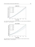
Bạn đang xem bản rút gọn của tài liệu. Xem và tải ngay bản đầy đủ của tài liệu tại đây (862.73 KB, 25 trang )
NonlinearAnalysisandDesignofPhase-LockedLoops 91
analysis of PLL, so readers should see mentioned papers and books and the references cited
therein.
2. Mathematical model of PLL
In this work three levels of PLL description are suggested:
1) the level of electronic realizations,
2) the level of phase and frequency relations between inputs and outputs in block diagrams,
3) the level of difference, differential and integro-differential equations.
The second level, involving the asymptotical analysis of high-frequency oscillations, is nec-
essary for the well-formed derivation of equations and for the passage to the third level of
description.
Consider a PLL on the first level (Fig. 1)
Fig. 1. Block diagram of PLL on the level of electronic realizations.
Here OSC
master
is a master oscillator, OSC
slave
is a slave (tunable) oscillator, which generate
high-frequency "almost harmonic oscillations"
f
j
(t) = A
j
sin(ω
j
(t)t + ψ
j
) j = 1, 2, (1)
where A
j
and ψ
j
are some numbers, ω
j
(t) are differentiable functions. Block
is a multiplier
of oscillations of f
1
(t) and f
2
(t) and the signal f
1
(t) f
2
(t) is its output. The relations between
the input ξ
(t) and the output σ(t) of linear filter have the form
σ
(t) = α
0
(t) +
t
0
γ(t − τ)ξ(τ) dτ. (2)
Here γ
(t) is an impulse transient function of filter, α
0
(t) is an exponentially damped function,
depending on the initial data of filter at the moment t
= 0. The electronic realizations of
generators, multipliers, and filters can be found in (Wolaver, 1991; Best, 2003; Chen, 2003;
Giannini & Leuzzi, 2004; Goldman, 2007; Razavi, 2001; Aleksenko, 2004). In the simplest
case it is assumed that the filter removes from the input the upper sideband with frequency
ω
1
(t) + ω
2
(t) but leaves the lower sideband ω
1
(t) − ω
2
(t) without change.
Now we reformulate the high-frequency property of oscillations f
j
(t) and essential assump-
tion that γ
(t) and ω
j
(t) are functions of "finite growth". For this purpose we consider the
great fixed time interval
[0, T], which can be partitioned into small intervals of the form
[τ, τ + δ], (τ ∈ [0, T]) such that the following relations
|γ(t) − γ(τ)| ≤ Cδ, |ω
j
(t) − ω
j
(τ)| ≤ Cδ,
∀t ∈ [ τ, τ + δ], ∀τ ∈ [0, T],
(3)
|ω
1
(τ) − ω
2
(τ)| ≤ C
1
, ∀τ ∈ [0, T], (4)
ω
j
(t) ≥ R, ∀t ∈ [0, T] (5)
are satisfied. Here we assume that the quantity δ is sufficiently small with respect to the fixed
numbers T, C, C
1
, the number R is sufficiently great with respect to the number δ. The latter
means that on the small intervals
[τ, τ + δ] the functions γ( t) and ω
j
(t) are "almost constants"
and the functions f
j
(t) rapidly oscillate as harmonic functions.
Consider two block diagrams shown in Fig. 2 and Fig. 3.
Fig. 2. Multiplier and filter.
Fig. 3. Phase detector and filter.
Here θ
j
(t) = ω
j
(t)t + ψ
j
are phases of the oscillations f
j
(t), PD is a nonlinear block with the
characteristic ϕ
(θ) (being called a phase detector or discriminator). The phases θ
j
(t) are the
inputs of PD block and the output is the function ϕ
(θ
1
(t) − θ
2
(t)). The shape of the phase
detector characteristic is based on the shape of input signals.
The signals f
1
(t) f
2
(t) and ϕ(θ
1
(t) −θ
2
(t)) are inputs of the same filters with the same impulse
transient function γ
(t). The filter outputs are the functions g(t) and G(t), respectively.
A classical PLL synthesis is based on the following result:
Theorem 1. (Viterbi, 1966) If conditions (3)–(5) are satisfied and we have
ϕ
(θ) =
1
2
A
1
A
2
cos θ,
then for the same initial data of filter, the following relation
|G(t) − g(t)| ≤ C
2
δ, ∀t ∈ [0, T]
is satisfied. Here C
2
is a certain number being independent of δ.
AUTOMATION&CONTROL-TheoryandPractice92
Proof of Theorem 1 (Leonov, 2006)
For t
∈ [0, T] we obviously have
g
(t) − G(t) =
=
t
0
γ(t − s)
A
1
A
2
sin
ω
1
(s)s + ψ
1
sin
ω
2
(s)s + ψ
2
−
−
ϕ
ω
1
(s)s − ω
2
(s)s + ψ
1
−ψ
2
ds
=
= −
A
1
A
2
2
t
0
γ(t − s)
cos
ω
1
(s) + ω
2
(s)
s
+ ψ
1
+ ψ
2
ds.
Consider the intervals
[kδ, (k + 1)δ], where k = 0, . . . , m and the number m is such that t ∈
[
mδ, (m + 1)δ]. From conditions (3)–(5) it follows that for any s ∈ [kδ, (k + 1)δ] the relations
γ
(t − s) = γ(t −kδ) + O(δ) (6)
ω
1
(s) + ω
2
(s) = ω
1
(kδ) + ω
2
(kδ) + O(δ) (7)
are valid on each interval
[kδ, (k + 1)δ]. Then by (7) for any s ∈ [kδ, (k + 1)δ] the estimate
cos
ω
1
(s) + ω
2
(s)
s
+ ψ
1
+ ψ
2
= cos
ω
1
(kδ) + ω
2
(kδ)
s
+ ψ
1
+ ψ
2
+ O(δ) (8)
is valid. Relations (6) and (8) imply that
t
0
γ(t − s)
cos
ω
1
(s) + ω
2
(s)
s
+ ψ
1
+ ψ
2
ds
=
=
m
∑
k=0
γ(t − kδ)
(k+1)δ
kδ
cos
ω
1
(kδ) + ω
2
(kδ)
s
+ ψ
1
+ ψ
2
ds
+ O(δ).
(9)
From (5) we have the estimate
(k+1)δ
kδ
cos
ω
1
(kδ) + ω
2
(kδ)
s
+ ψ
1
+ ψ
2
ds
= O(δ
2
)
and the fact that R is sufficiently great as compared with δ. Then
t
0
γ(t − s)
cos
ω
1
(s) + ω
2
(s)
s
+ ψ
1
+ ψ
2
ds
= O(δ).
Theorem 1 is completely proved.
Fig. 4. Block diagram of PLL on the level of phase relations
Thus, the outputs g
(t) and G(t) of two block diagrams in Fig. 2 and Fig. 3, respectively, differ
little from each other and we can pass (from a standpoint of the asymptotic with respect to δ)
to the following description level, namely to the second level of phase relations.
In this case a block diagram in Fig. 1 becomes the following block diagram (Fig. 4).
Consider now the high-frequency impulse oscillators, connected as in diagram in Fig. 1. Here
f
j
(t) = A
j
sign (sin(ω
j
(t)t + ψ
j
)). (10)
We assume, as before, that conditions (3)– (5) are satisfied.
Consider 2π-periodic function ϕ
(θ) of the form
ϕ
(θ) =
A
1
A
2
(1 + 2θ/π) for θ ∈ [−π, 0],
A
1
A
2
(1 −2θ/π) for θ ∈ [0, π].
(11)
and block diagrams in Fig. 2 and Fig. 3.
Theorem 2. (Leonov, 2006)
If conditions (3)–(5) are satisfied and the characteristic of phase detector ϕ
(θ) has the form (11), then
for the same initial data of filter the following relation
|G(t) − g(t)| ≤ C
3
δ, ∀t ∈ [0, T]
is satisfied. Here C
3
is a certain number being independent of δ.
Proof of Theorem 2
In this case we have
g
(t) − G(t) =
=
t
0
γ(t − s)
A
1
A
2
sign
sin
ω
1
(s)s + ψ
1
sin
ω
2
(s)s + ψ
2
−
−
ϕ
ω
1
(s)s − ω
2
(s)s + ψ
1
−ψ
2
ds.
NonlinearAnalysisandDesignofPhase-LockedLoops 93
Proof of Theorem 1 (Leonov, 2006)
For t
∈ [0, T] we obviously have
g
(t) − G(t) =
=
t
0
γ(t − s)
A
1
A
2
sin
ω
1
(s)s + ψ
1
sin
ω
2
(s)s + ψ
2
−
−
ϕ
ω
1
(s)s − ω
2
(s)s + ψ
1
−ψ
2
ds
=
= −
A
1
A
2
2
t
0
γ(t − s)
cos
ω
1
(s) + ω
2
(s)
s
+ ψ
1
+ ψ
2
ds.
Consider the intervals
[kδ, (k + 1)δ], where k = 0, . . . , m and the number m is such that t ∈
[
mδ, (m + 1)δ]. From conditions (3)–(5) it follows that for any s ∈ [kδ, (k + 1)δ] the relations
γ
(t − s) = γ(t −kδ) + O(δ) (6)
ω
1
(s) + ω
2
(s) = ω
1
(kδ) + ω
2
(kδ) + O(δ) (7)
are valid on each interval
[kδ, (k + 1)δ]. Then by (7) for any s ∈ [kδ, (k + 1)δ] the estimate
cos
ω
1
(s) + ω
2
(s)
s
+ ψ
1
+ ψ
2
= cos
ω
1
(kδ) + ω
2
(kδ)
s
+ ψ
1
+ ψ
2
+ O(δ) (8)
is valid. Relations (6) and (8) imply that
t
0
γ(t − s)
cos
ω
1
(s) + ω
2
(s)
s
+ ψ
1
+ ψ
2
ds
=
=
m
∑
k=0
γ(t − kδ)
(k+1)δ
kδ
cos
ω
1
(kδ) + ω
2
(kδ)
s
+ ψ
1
+ ψ
2
ds
+ O(δ).
(9)
From (5) we have the estimate
(k+1)δ
kδ
cos
ω
1
(kδ) + ω
2
(kδ)
s
+ ψ
1
+ ψ
2
ds
= O(δ
2
)
and the fact that R is sufficiently great as compared with δ. Then
t
0
γ(t − s)
cos
ω
1
(s) + ω
2
(s)
s
+ ψ
1
+ ψ
2
ds
= O(δ).
Theorem 1 is completely proved.
Fig. 4. Block diagram of PLL on the level of phase relations
Thus, the outputs g
(t) and G(t) of two block diagrams in Fig. 2 and Fig. 3, respectively, differ
little from each other and we can pass (from a standpoint of the asymptotic with respect to δ)
to the following description level, namely to the second level of phase relations.
In this case a block diagram in Fig. 1 becomes the following block diagram (Fig. 4).
Consider now the high-frequency impulse oscillators, connected as in diagram in Fig. 1. Here
f
j
(t) = A
j
sign (sin(ω
j
(t)t + ψ
j
)). (10)
We assume, as before, that conditions (3)– (5) are satisfied.
Consider 2π-periodic function ϕ
(θ) of the form
ϕ
(θ) =
A
1
A
2
(1 + 2θ/π) for θ ∈ [−π, 0],
A
1
A
2
(1 −2θ/π) for θ ∈ [0, π].
(11)
and block diagrams in Fig. 2 and Fig. 3.
Theorem 2. (Leonov, 2006)
If conditions (3)–(5) are satisfied and the characteristic of phase detector ϕ
(θ) has the form (11), then
for the same initial data of filter the following relation
|G(t) − g(t)| ≤ C
3
δ, ∀t ∈ [0, T]
is satisfied. Here C
3
is a certain number being independent of δ.
Proof of Theorem 2
In this case we have
g
(t) − G(t) =
=
t
0
γ(t − s)
A
1
A
2
sign
sin
ω
1
(s)s + ψ
1
sin
ω
2
(s)s + ψ
2
−
−
ϕ
ω
1
(s)s − ω
2
(s)s + ψ
1
−ψ
2
ds.
AUTOMATION&CONTROL-TheoryandPractice94
Partitioning the interval [0, t] into the intervals [kδ, (k + 1)δ] and making use of assumptions
(5) and (10), we replace the above integral with the following sum
m
∑
k=0
γ(t − kδ)
(k+1)δ
kδ
A
1
A
2
sign
cos
ω
1
(kδ)ω
2
(kδ)
kδ
+ ψ
1
−ψ
2
−
−
cos
ω
1
(kδ) + ω
2
(kδ)
s
+ ψ
1
+ ψ
2
ds
−
−
ϕ
ω
1
(kδ) −ω
2
(kδ)
kδ
+ ψ
1
−ψ
2
δ
.
The number m is chosen in such a way that t
∈ [mδ, (m + 1)δ]. Since (ω
1
(kδ) + ω
2
(kδ))δ 1,
the relation
(k+1)δ
kδ
A
1
A
2
sign
cos
ω
1
(kδ) −ω
2
(kδ)
kδ
+ ψ
1
−ψ
2
−
−
cos
ω
1
(kδ) + ω
2
(kδ)
s
+ ψ
1
+ ψ
2
ds
≈
≈
ϕ
ω
1
(kδ) −ω
2
(kδ)
kδ
+ ψ
1
−ψ
2
δ,
(12)
is satisfied. Here we use the relation
A
1
A
2
(k+1)δ
kδ
sign
cos α −cos
ωs + ψ
0
ds
≈ ϕ(α)δ
for ωδ
1, α ∈ [ −π, π], ψ
0
∈ R
1
.
Thus, Theorem 2 is completely proved.
Theorem 2 is a base for the synthesis of PLL with impulse oscillators. For the impulse clock
oscillators it permits one to consider two block diagrams simultaneously: on the level of elec-
tronic realization (Fig. 1) and on the level of phase relations (Fig. 4), where general principles
of the theory of phase synchronization can be used (Leonov & Seledzhi, 2005b; Kuznetsov et
al., 2006; Kuznetsov et al., 2007; Kuznetsov et al., 2008; Leonov, 2008).
3. Differential equations of PLL
Let us make a remark necessary for derivation of differential equations of PLL.
Consider a quantity
˙
θ
j
(t) = ω
j
(t) +
˙
ω
j
(t)t.
For the well-synthesized PLL such that it possesses the property of global stability, we have
exponential damping of the quantity
˙
ω
j
(t):
|
˙
ω
j
(t)| ≤ Ce
−αt
.
Here C and α are certain positive numbers being independent of t. Therefore, the quantity
˙
ω
j
(t)t is, as a rule, sufficiently small with respect to the number R (see conditions (3)– (5)).
From the above we can conclude that the following approximate relation
˙
θ
j
(t) ≈ ω
j
(t) is
valid. In deriving the differential equations of this PLL, we make use of a block diagram in
Fig. 4 and exact equality
˙
θ
j
(t) = ω
j
(t). (13)
Note that, by assumption, the control law of tunable oscillators is linear:
ω
2
(t) = ω
2
(0) + LG(t). (14)
Here ω
2
(0) is the initial frequency of tunable oscillator, L is a certain number, and G(t) is a
control signal, which is a filter output (Fig. 4). Thus, the equation of PLL is as follows
˙
θ
2
(t) = ω
2
(0) + L
α
0
(t) +
t
0
γ(t − τ)ϕ
θ
1
(τ) − θ
2
(τ)
dτ
.
Assuming that the master oscillator is such that ω
1
(t) ≡ ω
1
(0), we obtain the following rela-
tions for PLL
θ
1
(t) − θ
2
(t)
+ L
α
0
(t) +
t
0
γ(t − τ)ϕ
θ
1
(τ) − θ
2
(τ)
dτ
= ω
1
(0) − ω
2
(0). (15)
This is an equation of standard PLL. Note, that if the filter (2) is integrated with the transfer
function W
(p) = (p + α)
−1
˙
σ
+ ασ = ϕ(θ)
then for φ(θ) = cos(θ) instead of equation (15) from (13) and (14) we have
¨
˜
θ
+ α
˙
˜
θ + L sin
˜
θ = α
ω
1
(0) − ω
2
(0)
(16)
with
˜
θ
= θ
1
− θ
2
+
π
2
. So, if here phases of the input and output signals mutually shifted by
π/2 then the control signal G
(t) equals zero.
Arguing as above, we can conclude that in PLL it can be used the filters with transfer functions
of more general form
K
(p) = a + W(p),
where a is a certain number, W
(p) is a proper fractional rational function. In this case in place
of equation (15) we have
θ
1
(t) − θ
2
(t)
+ L
aϕ
θ
1
(t) − θ
2
(t)
+ α
0
(t) +
t
0
γ(t − τ)ϕ
θ
1
(τ) − θ
2
(τ)
dτ
=
=
ω
1
(0) − ω
2
(0).
(17)
In the case when the transfer function of the filter a
+ W(p) is non-degenerate, i.e. its numer-
ator and denominator do not have common roots, equation (17) is equivalent to the following
system of differential equations
˙
z
= Az + bψ(σ)
˙
σ
= c
∗
z + ρψ(σ).
(18)
NonlinearAnalysisandDesignofPhase-LockedLoops 95
Partitioning the interval [0, t] into the intervals [kδ, (k + 1)δ] and making use of assumptions
(5) and (10), we replace the above integral with the following sum
m
∑
k=0
γ(t − kδ)
(k+1)δ
kδ
A
1
A
2
sign
cos
ω
1
(kδ)ω
2
(kδ)
kδ
+ ψ
1
−ψ
2
−
−
cos
ω
1
(kδ) + ω
2
(kδ)
s
+ ψ
1
+ ψ
2
ds
−
−
ϕ
ω
1
(kδ) −ω
2
(kδ)
kδ
+ ψ
1
−ψ
2
δ
.
The number m is chosen in such a way that t
∈ [mδ, (m + 1)δ]. Since (ω
1
(kδ) + ω
2
(kδ))δ 1,
the relation
(k+1)δ
kδ
A
1
A
2
sign
cos
ω
1
(kδ) −ω
2
(kδ)
kδ
+ ψ
1
−ψ
2
−
−
cos
ω
1
(kδ) + ω
2
(kδ)
s
+ ψ
1
+ ψ
2
ds
≈
≈
ϕ
ω
1
(kδ) −ω
2
(kδ)
kδ
+ ψ
1
−ψ
2
δ,
(12)
is satisfied. Here we use the relation
A
1
A
2
(k+1)δ
kδ
sign
cos α −cos
ωs + ψ
0
ds
≈ ϕ(α)δ
for ωδ
1, α ∈ [ −π, π], ψ
0
∈ R
1
.
Thus, Theorem 2 is completely proved.
Theorem 2 is a base for the synthesis of PLL with impulse oscillators. For the impulse clock
oscillators it permits one to consider two block diagrams simultaneously: on the level of elec-
tronic realization (Fig. 1) and on the level of phase relations (Fig. 4), where general principles
of the theory of phase synchronization can be used (Leonov & Seledzhi, 2005b; Kuznetsov et
al., 2006; Kuznetsov et al., 2007; Kuznetsov et al., 2008; Leonov, 2008).
3. Differential equations of PLL
Let us make a remark necessary for derivation of differential equations of PLL.
Consider a quantity
˙
θ
j
(t) = ω
j
(t) +
˙
ω
j
(t)t.
For the well-synthesized PLL such that it possesses the property of global stability, we have
exponential damping of the quantity
˙
ω
j
(t):
|
˙
ω
j
(t)| ≤ Ce
−αt
.
Here C and α are certain positive numbers being independent of t. Therefore, the quantity
˙
ω
j
(t)t is, as a rule, sufficiently small with respect to the number R (see conditions (3)– (5)).
From the above we can conclude that the following approximate relation
˙
θ
j
(t) ≈ ω
j
(t) is
valid. In deriving the differential equations of this PLL, we make use of a block diagram in
Fig. 4 and exact equality
˙
θ
j
(t) = ω
j
(t). (13)
Note that, by assumption, the control law of tunable oscillators is linear:
ω
2
(t) = ω
2
(0) + LG(t). (14)
Here ω
2
(0) is the initial frequency of tunable oscillator, L is a certain number, and G(t) is a
control signal, which is a filter output (Fig. 4). Thus, the equation of PLL is as follows
˙
θ
2
(t) = ω
2
(0) + L
α
0
(t) +
t
0
γ(t − τ)ϕ
θ
1
(τ) − θ
2
(τ)
dτ
.
Assuming that the master oscillator is such that ω
1
(t) ≡ ω
1
(0), we obtain the following rela-
tions for PLL
θ
1
(t) − θ
2
(t)
+ L
α
0
(t) +
t
0
γ(t − τ)ϕ
θ
1
(τ) − θ
2
(τ)
dτ
= ω
1
(0) − ω
2
(0). (15)
This is an equation of standard PLL. Note, that if the filter (2) is integrated with the transfer
function W
(p) = (p + α)
−1
˙
σ
+ ασ = ϕ(θ)
then for φ(θ) = cos(θ) instead of equation (15) from (13) and (14) we have
¨
˜
θ
+ α
˙
˜
θ + L sin
˜
θ = α
ω
1
(0) − ω
2
(0)
(16)
with
˜
θ
= θ
1
− θ
2
+
π
2
. So, if here phases of the input and output signals mutually shifted by
π/2 then the control signal G
(t) equals zero.
Arguing as above, we can conclude that in PLL it can be used the filters with transfer functions
of more general form
K
(p) = a + W(p),
where a is a certain number, W
(p) is a proper fractional rational function. In this case in place
of equation (15) we have
θ
1
(t) − θ
2
(t)
+ L
aϕ
θ
1
(t) − θ
2
(t)
+ α
0
(t) +
t
0
γ(t − τ)ϕ
θ
1
(τ) − θ
2
(τ)
dτ
=
=
ω
1
(0) − ω
2
(0).
(17)
In the case when the transfer function of the filter a
+ W(p) is non-degenerate, i.e. its numer-
ator and denominator do not have common roots, equation (17) is equivalent to the following
system of differential equations
˙
z
= Az + bψ(σ)
˙
σ
= c
∗
z + ρψ(σ).
(18)
AUTOMATION&CONTROL-TheoryandPractice96
Here σ = θ
1
−θ
2
, A is a constant (n ×n)-matrix, b and c are constant (n)-vectors, ρ is a number,
and ψ
(σ) is 2π-periodic function, satisfying the relations:
ρ
= −aL,
W
(p) = L
−1
c
∗
(A − pI)
−1
b,
ψ
(σ) = ϕ(σ) −
ω
1
(0) − ω
2
(0)
L(a + W(0))
.
The discrete phase-locked loops obey similar equations
z
(t + 1) = Az(t) + bψ(σ(t))
σ(t + 1) = σ(t) + c
∗
z(t) + ρψ(σ(t)),
(19)
where t
∈ Z, Z is a set of integers. Equations (18) and (19) describe the so-called standard
PLLs (Shakhgil’dyan & Lyakhovkin, 1972; Leonov, 2001). Note that there exist many other
modifications of PLLs and some of them are considered below.
4. Mathematical analysis methods of PLL
The theory of phase synchronization was developed in the second half of the last century on
the basis of three applied theories: theory of synchronous and induction electrical motors, the-
ory of auto-synchronization of the unbalanced rotors, theory of phase-locked loops. Its main
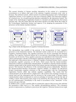
principle is in consideration of the problem of phase synchronization at three levels: (i) at the
level of mechanical, electromechanical, or electronic models, (ii) at the level of phase relations,
and (iii) at the level of differential, difference, integral, and integro-differential equations. In
this case the difference of oscillation phases is transformed into the control action, realizing
synchronization. These general principles gave impetus to creation of universal methods for
studying the phase synchronization systems. Modification of the direct Lyapunov method
with the construction of periodic Lyapunov-like functions, the method of positively invari-
ant cone grids, and the method of nonlocal reduction turned out to be most effective. The
last method, which combines the elements of the direct Lyapunov method and the bifurca-
tion theory, allows one to extend the classical results of F. Tricomi and his progenies to the
multidimensional dynamical systems.
4.1 Method of periodic Lyapunov functions
Here we formulate the extension of the Barbashin–Krasovskii theorem to dynamical systems
with a cylindrical phase space (Barbashin & Krasovskii, 1952). Consider a differential inclu-
sion
˙
x
∈ f (x), x ∈ R
n
, t ∈ R
1
, (20)
where f
(x) is a semicontinuous vector function whose values are the bounded closed convex
set f
(x) ⊂ R
n
. Here R
n
is an n-dimensional Euclidean space. Recall the basic definitions of
the theory of differential inclusions.
Definition 1. We say that U
ε
(Ω) is an ε-neighbourhood of the set Ω if
U
ε
(Ω) = {x | inf
y∈Ω
|x − y| < ε},
where
|· | is an Euclidean norm in R
n
.
Definition 2. A function f (x) is called semicontinuous at a point x if for any ε > 0 there exists a
number δ
(x, ε) > 0 such that the following containment holds:
f
(y) ∈ U
ε
( f (x)), ∀y ∈ U
δ
(x).
Definition 3. A vector function x
(t) is called a solution of differential inclusion if it is absolutely
continuous and for the values of t, at which the derivative
˙
x
(t) exists, the inclusion
˙
x
(t) ∈ f (x(t))
holds.
Under the above assumptions on the function f
(x), the theorem on the existence and con-
tinuability of solution of differential inclusion (20) is valid (Yakubovich et al., 2004). Now we
assume that the linearly independent vectors d
1
, . . . , d
m
satisfy the following relations:
f
(x + d
j
) = f (x), ∀x ∈ R
n
. (21)
Usually, d
∗
j
x is called the phase or angular coordinate of system (20). Since property (21)
allows us to introduce a cylindrical phase space (Yakubovich et al., 2004), system (20) with
property (21) is often called a system with cylindrical phase space.
The following theorem is an extension of the well–known Barbashin–Krasovskii theorem to
differential inclusions with a cylindrical phase space.
Theorem 3. Suppose that there exists a continuous function V
(x) : R
n
→ R
1
such that the following
conditions hold:
1) V
(x + d
j
) = V(x), ∀x ∈ R
n
, ∀j = 1, . . . , m;
2) V
(x) +
m
∑
j=1
(d
∗
j
x)
2
→ ∞ as |x| → ∞;
3) for any solution x
(t) of inclusion (20) the function V(x(t)) is nonincreasing;
4) if V
(x(t)) ≡ V(x(0)), then x(t) is an equilibrium state.
Then any solution of inclusion (20) tends to stationary set as t
→ +∞.
Recall that the tendency of solution to the stationary set Λ as t means that
lim
t→+∞
inf
z∈Λ
|z − x(t)| = 0.
A proof of Theorem 3 can be found in (Yakubovich et al., 2004).
4.2 Method of positively invariant cone grids. An analog of circular criterion
This method was proposed independently in the works (Leonov, 1974; Noldus, 1977). It is suf-
ficiently universal and "fine" in the sense that here only two properties of system are used such
as the availability of positively invariant one-dimensional quadratic cone and the invariance
of field of system (20) under shifts by the vector d
j
(see (21)).
Here we consider this method for more general nonautonomous case
˙
x
= F(t, x), x ∈ R
n
, t ∈ R
1
,
where the identities F
(t, x + d
j
) = F(t, x) are valid ∀x ∈ R
n
, ∀t ∈ R
1
for the linearly inde-
pendent vectors d
j
∈ R
n
(j = 1, , m). Let x(t) = x(t , t
0
, x
0
) is a solution of the system such
that x
(t
0
, t
0
, x
0
) = x
0
.
NonlinearAnalysisandDesignofPhase-LockedLoops 97
Here σ = θ
1
−θ
2
, A is a constant (n ×n)-matrix, b and c are constant (n)-vectors, ρ is a number,
and ψ
(σ) is 2π-periodic function, satisfying the relations:
ρ
= −aL,
W
(p) = L
−1
c
∗
(A − pI)
−1
b,
ψ
(σ) = ϕ(σ) −
ω
1
(0) − ω
2
(0)
L(a + W(0))
.
The discrete phase-locked loops obey similar equations
z
(t + 1) = Az(t) + bψ(σ(t))
σ(t + 1) = σ(t) + c
∗
z(t) + ρψ(σ(t)),
(19)
where t
∈ Z, Z is a set of integers. Equations (18) and (19) describe the so-called standard
PLLs (Shakhgil’dyan & Lyakhovkin, 1972; Leonov, 2001). Note that there exist many other
modifications of PLLs and some of them are considered below.
4. Mathematical analysis methods of PLL
The theory of phase synchronization was developed in the second half of the last century on
the basis of three applied theories: theory of synchronous and induction electrical motors, the-
ory of auto-synchronization of the unbalanced rotors, theory of phase-locked loops. Its main
principle is in consideration of the problem of phase synchronization at three levels: (i) at the
level of mechanical, electromechanical, or electronic models, (ii) at the level of phase relations,
and (iii) at the level of differential, difference, integral, and integro-differential equations. In
this case the difference of oscillation phases is transformed into the control action, realizing
synchronization. These general principles gave impetus to creation of universal methods for
studying the phase synchronization systems. Modification of the direct Lyapunov method
with the construction of periodic Lyapunov-like functions, the method of positively invari-
ant cone grids, and the method of nonlocal reduction turned out to be most effective. The
last method, which combines the elements of the direct Lyapunov method and the bifurca-
tion theory, allows one to extend the classical results of F. Tricomi and his progenies to the
multidimensional dynamical systems.
4.1 Method of periodic Lyapunov functions
Here we formulate the extension of the Barbashin–Krasovskii theorem to dynamical systems
with a cylindrical phase space (Barbashin & Krasovskii, 1952). Consider a differential inclu-
sion
˙
x
∈ f (x), x ∈ R
n
, t ∈ R
1
, (20)
where f
(x) is a semicontinuous vector function whose values are the bounded closed convex
set f
(x) ⊂ R
n
. Here R
n
is an n-dimensional Euclidean space. Recall the basic definitions of
the theory of differential inclusions.
Definition 1. We say that U
ε
(Ω) is an ε-neighbourhood of the set Ω if
U
ε
(Ω) = {x | inf
y∈Ω
|x − y| < ε},
where
|· | is an Euclidean norm in R
n
.
Definition 2. A function f (x) is called semicontinuous at a point x if for any ε > 0 there exists a
number δ
(x, ε) > 0 such that the following containment holds:
f
(y) ∈ U
ε
( f (x)), ∀y ∈ U
δ
(x).
Definition 3. A vector function x
(t) is called a solution of differential inclusion if it is absolutely
continuous and for the values of t, at which the derivative
˙
x
(t) exists, the inclusion
˙
x
(t) ∈ f (x(t))
holds.
Under the above assumptions on the function f
(x), the theorem on the existence and con-
tinuability of solution of differential inclusion (20) is valid (Yakubovich et al., 2004). Now we
assume that the linearly independent vectors d
1
, . . . , d
m
satisfy the following relations:
f
(x + d
j
) = f (x), ∀x ∈ R
n
. (21)
Usually, d
∗
j
x is called the phase or angular coordinate of system (20). Since property (21)
allows us to introduce a cylindrical phase space (Yakubovich et al., 2004), system (20) with
property (21) is often called a system with cylindrical phase space.
The following theorem is an extension of the well–known Barbashin–Krasovskii theorem to
differential inclusions with a cylindrical phase space.
Theorem 3. Suppose that there exists a continuous function V
(x) : R
n
→ R
1
such that the following
conditions hold:
1) V
(x + d
j
) = V(x), ∀x ∈ R
n
, ∀j = 1, . . . , m;
2) V
(x) +
m
∑
j=1
(d
∗
j
x)
2
→ ∞ as |x| → ∞;
3) for any solution x
(t) of inclusion (20) the function V(x(t)) is nonincreasing;
4) if V
(x(t)) ≡ V(x(0)), then x(t) is an equilibrium state.
Then any solution of inclusion (20) tends to stationary set as t
→ +∞.
Recall that the tendency of solution to the stationary set Λ as t means that
lim
t→+∞
inf
z∈Λ
|z − x(t)| = 0.
A proof of Theorem 3 can be found in (Yakubovich et al., 2004).
4.2 Method of positively invariant cone grids. An analog of circular criterion
This method was proposed independently in the works (Leonov, 1974; Noldus, 1977). It is suf-
ficiently universal and "fine" in the sense that here only two properties of system are used such
as the availability of positively invariant one-dimensional quadratic cone and the invariance
of field of system (20) under shifts by the vector d
j
(see (21)).
Here we consider this method for more general nonautonomous case
˙
x
= F(t, x), x ∈ R
n
, t ∈ R
1
,
where the identities F
(t, x + d
j
) = F(t, x) are valid ∀x ∈ R
n
, ∀t ∈ R
1
for the linearly inde-
pendent vectors d
j
∈ R
n
(j = 1, , m). Let x(t) = x(t , t
0
, x
0
) is a solution of the system such
that x
(t
0
, t
0
, x
0
) = x
0
.
AUTOMATION&CONTROL-TheoryandPractice98
We assume that such a cone of the form Ω = {x
∗
Hx ≤ 0}, where H is a symmetrical matrix
such that one eigenvalue is negative and all the rest are positive, is positively invariant. The
latter means that on the boundary of cone ∂Ω
= {xHx = 0} the relation
˙
V
(x(t)) < 0
is satisfied for all x
(t) such that {x(t) = 0, x(t) ∈ ∂Ω} (Fig. 5).
Fig. 5. Positively invariant cone.
By the second property, namely the invariance of vector field under shift by the vectors kd
j
,
k
∈ Z, we multiply the cone in the following way
Ω
k
= {(x − kd
j
)H(x −kd
j
) ≤ 0}.
Since it is evident that for the cones Ω
k
the property of positive invariance holds true, we
obtain a positively invariant cone grid shown in Fig. 6. As can be seen from this figure, all the
Fig. 6. Positively invariant cone grid.
solutions x
(t, t
0
, x
0
) of system, having these two properties, are bounded on [t
0
, +∞).
If the cone Ω has only one point of intersection with the hyperplane
{d
∗
j
x = 0} and all solu-
tions x
(t), for which at the time t the inequality
x
(t)
∗
Hx(t) ≥ 0
is satisfied, have property
˙
V
(x(t)) ≤ −ε|x(t)|
2
(here ε is a positive number), then from Fig. 6 it
is clear that the system is Lagrange stable (all solutions are bounded on the interval
[0, +∞)).
Thus, the proposed method is simple and universal. By the Yakubovich–Kalman frequency
theorem it becomes practically efficient (Gelig et al., 1978; Yakubovich et al., 2004).
Consider, for example, the system
˙
x
= Px + qϕ(t, σ), σ = r
∗
x, (22)
where P is a constant singular n
× n-matrix, q and r are constant n-dimensional vectors, and
ϕ
(t, σ) is a continuous 2π-periodic in σ function R
1
× R
1
→ R
1
, satisfying the relations
µ
1
≤
ϕ(t, σ)
σ
≤ µ
2
, ∀t ∈ R
1
, ∀σ = 0, ϕ(t, 0) = 0.
Here µ
1
and µ
2
are some numbers, which by virtue of periodicity of ϕ(t, σ) in σ, without loss
of generality, can be assumed to be negative, µ
1
< 0, and positive, µ
2
> 0, respectively.
We introduce the transfer function of system (22)
χ
(p) = r
∗
(P − pI)
−1
q,
which is assumed to be nondegenerate. Consider now quadratic forms V
(x) = x
∗
Hx and
G
(x, ξ) = 2x
∗
H[ (P + λI)x + qξ] + (µ
−1
2
ξ −r
∗
x)(µ
−1
1
ξ −r
∗
x),
where λ is a positive number.
By the Yakubovich–Kalman theorem, for the existence of the symmetrical matrix H with one
negative and n
−1 positive eigenvalues and such that the inequality G(x, ξ) < 0, ∀x ∈ R
n
, ξ ∈
R
1
, x = 0 is satisfied, it is sufficient that
(C1) the matrix
(P + λI) has (n −1) eigenvalues with negative real part and
(C2) the frequency inequality
µ
−1
1
µ
−1
2
+ (µ
−1
1
+ µ
−1
2
)Reχ(iω − λ) + |χ(iω − λ)|
2
< 0, ∀ω ∈ R
1
is satisfied.
It is easy to see that the condition G
(x, ξ) < 0, ∀ x = 0, ∀ξ implies the relation
˙
V
x
(t)
+ 2λ V
x(t)
< 0, ∀x(t) = 0.
This inequality assures the positive invariance of the considered cone Ω.
Thus, we obtain the following analog of the well-known circular criterion.
Theorem 4. ( Leonov, 1974; Gelig et al., 1978; Yakubovich et al., 2004)
If there exists a positive number λ such that the above conditions (C1) and (C2) are satisfied, then any
solution x
(t, t
0
, x
0
) of system (22) is bounded on the interval (t
0
, +∞).
A more detailed proof of this fact can be found in (Leonov & Smirnova 2000; Gelig et al., 1978;
Yakubovich et al., 2004). We note that this theorem is also true under the condition of nonstrict
inequality in (C2) and in the cases when µ
1
= −∞ or µ
2
= +∞ (Leonov & Smirnova 2000;
Gelig et al., 1978; Yakubovich et al., 2004).
We apply now an analog of the circular criterion, formulated with provision for the above
remark, to the simplest case of the second-order equation
¨
θ
+ α
˙
θ + ϕ(t, θ) = 0, (23)
NonlinearAnalysisandDesignofPhase-LockedLoops 99
We assume that such a cone of the form Ω = {x
∗
Hx ≤ 0}, where H is a symmetrical matrix
such that one eigenvalue is negative and all the rest are positive, is positively invariant. The
latter means that on the boundary of cone ∂Ω
= {xHx = 0} the relation
˙
V
(x(t)) < 0
is satisfied for all x
(t) such that {x(t) = 0, x(t) ∈ ∂Ω} (Fig. 5).
Fig. 5. Positively invariant cone.
By the second property, namely the invariance of vector field under shift by the vectors kd
j
,
k
∈ Z, we multiply the cone in the following way
Ω
k
= {(x − kd
j
)H(x −kd
j
) ≤ 0}.
Since it is evident that for the cones Ω
k
the property of positive invariance holds true, we
obtain a positively invariant cone grid shown in Fig. 6. As can be seen from this figure, all the
Fig. 6. Positively invariant cone grid.
solutions x
(t, t
0
, x
0
) of system, having these two properties, are bounded on [t
0
, +∞).
If the cone Ω has only one point of intersection with the hyperplane
{d
∗
j
x = 0} and all solu-
tions x
(t), for which at the time t the inequality
x
(t)
∗
Hx(t) ≥ 0
is satisfied, have property
˙
V
(x(t)) ≤ −ε|x(t)|
2
(here ε is a positive number), then from Fig. 6 it
is clear that the system is Lagrange stable (all solutions are bounded on the interval
[0, +∞)).
Thus, the proposed method is simple and universal. By the Yakubovich–Kalman frequency
theorem it becomes practically efficient (Gelig et al., 1978; Yakubovich et al., 2004).
Consider, for example, the system
˙
x
= Px + qϕ(t, σ), σ = r
∗
x, (22)
where P is a constant singular n
× n-matrix, q and r are constant n-dimensional vectors, and
ϕ
(t, σ) is a continuous 2π-periodic in σ function R
1
× R
1
→ R
1
, satisfying the relations
µ
1
≤
ϕ(t, σ)
σ
≤ µ
2
, ∀t ∈ R
1
, ∀σ = 0, ϕ(t, 0) = 0.
Here µ
1
and µ
2
are some numbers, which by virtue of periodicity of ϕ(t, σ) in σ, without loss
of generality, can be assumed to be negative, µ
1
< 0, and positive, µ
2
> 0, respectively.
We introduce the transfer function of system (22)
χ
(p) = r
∗
(P − pI)
−1
q,
which is assumed to be nondegenerate. Consider now quadratic forms V
(x) = x
∗
Hx and
G
(x, ξ) = 2x
∗
H[ (P + λI)x + qξ] + (µ
−1
2
ξ −r
∗
x)(µ
−1
1
ξ −r
∗
x),
where λ is a positive number.
By the Yakubovich–Kalman theorem, for the existence of the symmetrical matrix H with one
negative and n
−1 positive eigenvalues and such that the inequality G(x, ξ) < 0, ∀x ∈ R
n
, ξ ∈
R
1
, x = 0 is satisfied, it is sufficient that
(C1) the matrix
(P + λI) has (n −1) eigenvalues with negative real part and
(C2) the frequency inequality
µ
−1
1
µ
−1
2
+ (µ
−1
1
+ µ
−1
2
)Reχ(iω − λ) + |χ(iω − λ)|
2
< 0, ∀ω ∈ R
1
is satisfied.
It is easy to see that the condition G
(x, ξ) < 0, ∀ x = 0, ∀ξ implies the relation
˙
V
x
(t)
+ 2λ V
x(t)
< 0, ∀x(t) = 0.
This inequality assures the positive invariance of the considered cone Ω.
Thus, we obtain the following analog of the well-known circular criterion.
Theorem 4. ( Leonov, 1974; Gelig et al., 1978; Yakubovich et al., 2004)
If there exists a positive number λ such that the above conditions (C1) and (C2) are satisfied, then any
solution x
(t, t
0
, x
0
) of system (22) is bounded on the interval (t
0
, +∞).
A more detailed proof of this fact can be found in (Leonov & Smirnova 2000; Gelig et al., 1978;
Yakubovich et al., 2004). We note that this theorem is also true under the condition of nonstrict
inequality in (C2) and in the cases when µ
1
= −∞ or µ
2
= +∞ (Leonov & Smirnova 2000;
Gelig et al., 1978; Yakubovich et al., 2004).
We apply now an analog of the circular criterion, formulated with provision for the above
remark, to the simplest case of the second-order equation
¨
θ
+ α
˙
θ + ϕ(t, θ) = 0, (23)
AUTOMATION&CONTROL-TheoryandPractice100
where α is a positive parameter (equation (16) can be transformed into (23) by
˜
θ = θ +
arcsin
α
ω
1
(0) − ω
2
(0)
/L
). This equation can be represented as system (22) with n
= 2
and the transfer function
χ
(p) =
1
p(p + α)
.
Obviously, condition (C1) of theorem takes the form λ
∈ (0, α) and for µ
1
= −∞ and µ
2
=
α
2
/4 condition (C2) is equivalent to the inequality
−ω
2
+ λ
2
−αλ + α
2
/4 ≤ 0, ∀ω ∈ R
1
.
This inequality is satisfied for λ
= α/2. Thus, if in equation (23) the function ϕ(t, θ) is periodic
with respect to θ and satisfies the inequality
ϕ
(t, θ)
θ
≤
α
2
4
, (24)
then any its solution θ
(t) is bounded on (t
0
, +∞).
It is easily seen that for ϕ
(t, θ) ≡ ϕ(θ) (i.e. ϕ(t, θ) is independent of t) equation (23) is di-
chotomic. It follows that in the autonomous case if relation (24) is satisfied, then any solution
of (23) tends to certain equilibrium state as t
→ +∞.
Here we have interesting analog of notion of absolute stability for phase synchronization sys-
tems. If system (22) is absolutely stable under the condition that for any nonlinearity ϕ from
the sector
[µ
1
, µ
2
] any its solution tends to certain equilibrium state, then for equation (23)
with ϕ
(t, θ) ≡ ϕ(θ) this sector is (−∞, α
2
/4].
At the same time, in the classical theory of absolute stability (without the assumption that ϕ is
periodic), for ϕ
(t, θ) ≡ ϕ(θ) we have two sectors: the sector of absolute stability (0, +∞) and
the sector of absolute instability
(−∞, 0).
Thus, the periodicity alone of ϕ allows one to cover a part of sector of absolute stability and a
complete sector of absolute instability:
(−∞, α
2
/4] ⊃ (−∞, 0) ∪ (0, α
2
/4] (see Fig. 7).
Fig. 7. Sectors of stability and instability.
More complex examples of using the analog of circular criterion can be found in (Leonov &
Smirnova 2000; Gelig et al., 1978; Yakubovich et al., 2004).
4.3 Method of nonlocal reduction
We describe the main stages of extending the theorems of Tricomi and his progenies, obtained
for the equation
¨
θ
+ α
˙
θ + ψ(θ) = 0, (25)
to systems of higher dimensions.
Consider first the system
˙
z
= Az + bψ(σ)
˙
σ
= c
∗
z + ρψ(σ),
(26)
describing a standard PLL. We assume, as usual, that ψ
(σ) is 2π-periodic, A is a stable n × n-
matrix, b and c are constant n-vectors, and ρ is a number.
Consider the case when any solution of equation (25) or its equivalent system
˙
η
= −αη − ψ(θ)
˙
θ
= η
(27)
tends to the equilibrium state as t
→ +∞. In this case it is possible to demonstrate (Barbashin
& Tabueva, 1969) that for the equation
dη
dθ
=
−
αη −ψ(θ)
η
(28)
equivalent to (27) there exists a solution η
(θ) such that η(θ
0
) = 0, η (θ) = 0, ∀θ = θ
0
,
lim
θ→+∞
η(θ) = − ∞, lim
θ→−∞
η(θ) = + ∞. (29)
Here θ
0
is a number such that ψ(θ
0
) = 0, ψ
(θ
0
) < 0.
We consider now the function
V
(z, σ) = z
∗
Hz −
1
2
η
(σ)
2
,
which induces the cone Ω
= {V(z, σ) ≤ 0} in the phase space {z, σ}. This is a generaliza-
tion of quadratic cone shown in Fig. 5. We prove that under certain conditions this cone is
positively invariant. Consider the expression
dV
dt
+ 2λ V = 2z
∗
H
[
(
A + λI)z + bψ(σ)
]
−λη(σ)
2
−η(σ)
dη(σ)
dσ
(c
∗
z + ρψ(σ)) =
=
2z
∗
H
[
(
A + λI)z + bψ(σ)
]
−λη(σ)
2
+ ψ(σ)(c
∗
z + ρψ(σ)) + αη(σ)(c
∗
z + ρψ(σ)).
Here we make use of the fact that η
(σ) satisfies equation (28).
We note that if the frequency inequalities
Re W
(iω − λ) − ε|K(iω − λ)|
2
> 0,
lim
ω→∞
ω
2
(Re K(iω −λ) − ε|K(iω − λ)|
2
) > 0,
(30)
where K
(p) = c
∗
(A − pI)
−1
b − ρ, are satisfied, then by the Yakubovich–Kalman frequency
theorem there exists H such that for ξ and all z
= 0 the following relation
2z
∗
H[ (A + λI)z + bξ] + ξ(c
∗
z + ρξ) + ε|(c
∗
z + ρξ)|
2
< 0
NonlinearAnalysisandDesignofPhase-LockedLoops 101
where α is a positive parameter (equation (16) can be transformed into (23) by
˜
θ = θ +
arcsin
α
ω
1
(0) − ω
2
(0)
/L
). This equation can be represented as system (22) with n
= 2
and the transfer function
χ
(p) =
1
p
(p + α)
.
Obviously, condition (C1) of theorem takes the form λ
∈ (0, α) and for µ
1
= −∞ and µ
2
=
α
2
/4 condition (C2) is equivalent to the inequality
−ω
2
+ λ
2
−αλ + α
2
/4 ≤ 0, ∀ω ∈ R
1
.
This inequality is satisfied for λ
= α/2. Thus, if in equation (23) the function ϕ(t, θ) is periodic
with respect to θ and satisfies the inequality
ϕ
(t, θ)
θ
≤
α
2
4
, (24)
then any its solution θ
(t) is bounded on (t
0
, +∞).
It is easily seen that for ϕ
(t, θ) ≡ ϕ(θ) (i.e. ϕ(t, θ) is independent of t) equation (23) is di-
chotomic. It follows that in the autonomous case if relation (24) is satisfied, then any solution
of (23) tends to certain equilibrium state as t
→ +∞.
Here we have interesting analog of notion of absolute stability for phase synchronization sys-
tems. If system (22) is absolutely stable under the condition that for any nonlinearity ϕ from
the sector
[µ
1
, µ
2
] any its solution tends to certain equilibrium state, then for equation (23)
with ϕ
(t, θ) ≡ ϕ(θ) this sector is (−∞, α
2
/4].
At the same time, in the classical theory of absolute stability (without the assumption that ϕ is
periodic), for ϕ
(t, θ) ≡ ϕ(θ) we have two sectors: the sector of absolute stability (0, +∞) and
the sector of absolute instability
(−∞, 0).
Thus, the periodicity alone of ϕ allows one to cover a part of sector of absolute stability and a
complete sector of absolute instability:
(−∞, α
2
/4] ⊃ (−∞, 0) ∪ (0, α
2
/4] (see Fig. 7).
Fig. 7. Sectors of stability and instability.
More complex examples of using the analog of circular criterion can be found in (Leonov &
Smirnova 2000; Gelig et al., 1978; Yakubovich et al., 2004).
4.3 Method of nonlocal reduction
We describe the main stages of extending the theorems of Tricomi and his progenies, obtained
for the equation
¨
θ
+ α
˙
θ + ψ(θ) = 0, (25)
to systems of higher dimensions.
Consider first the system
˙
z
= Az + bψ(σ)
˙
σ
= c
∗
z + ρψ(σ),
(26)
describing a standard PLL. We assume, as usual, that ψ
(σ) is 2π-periodic, A is a stable n × n-
matrix, b and c are constant n-vectors, and ρ is a number.
Consider the case when any solution of equation (25) or its equivalent system
˙
η
= −αη − ψ(θ)
˙
θ
= η
(27)
tends to the equilibrium state as t
→ +∞. In this case it is possible to demonstrate (Barbashin
& Tabueva, 1969) that for the equation
dη
dθ
=
−
αη −ψ(θ)
η
(28)
equivalent to (27) there exists a solution η
(θ) such that η(θ
0
) = 0, η (θ) = 0, ∀θ = θ
0
,
lim
θ→+∞
η(θ) = − ∞, lim
θ→−∞
η(θ) = + ∞. (29)
Here θ
0
is a number such that ψ(θ
0
) = 0, ψ
(θ
0
) < 0.
We consider now the function
V
(z, σ) = z
∗
Hz −
1
2
η
(σ)
2
,
which induces the cone Ω
= {V(z, σ) ≤ 0} in the phase space {z, σ}. This is a generaliza-
tion of quadratic cone shown in Fig. 5. We prove that under certain conditions this cone is
positively invariant. Consider the expression
dV
dt
+ 2λ V = 2z
∗
H
[
(
A + λI)z + bψ(σ)
]
−λη(σ)
2
−η(σ)
dη(σ)
dσ
(c
∗
z + ρψ(σ)) =
=
2z
∗
H
[
(
A + λI)z + bψ(σ)
]
−λη(σ)
2
+ ψ(σ)(c
∗
z + ρψ(σ)) + αη(σ)(c
∗
z + ρψ(σ)).
Here we make use of the fact that η
(σ) satisfies equation (28).
We note that if the frequency inequalities
Re W
(iω − λ) − ε|K(iω − λ)|
2
> 0,
lim
ω→∞
ω
2
(Re K(iω −λ) − ε|K(iω − λ)|
2
) > 0,
(30)
where K
(p) = c
∗
(A − pI)
−1
b − ρ, are satisfied, then by the Yakubovich–Kalman frequency
theorem there exists H such that for ξ and all z
= 0 the following relation
2z
∗
H[ (A + λI)z + bξ] + ξ(c
∗
z + ρξ) + ε|(c
∗
z + ρξ)|
2
< 0
AUTOMATION&CONTROL-TheoryandPractice102
is valid. Here ε is a positive number. If A + λI is a stable matrix, then H > 0.
Thus, if
(A + λI) is stable, (30) and α
2
≤ 4λε are satisfied, then we have
dV
dt
+ 2λ V < 0, ∀z(t) = 0
and, therefore, Ω is a positively invariant cone.
We can make a breeding of the cones Ω
k
= {z
∗
Hz −
1
2
η
k
(σ)
2
≤ 0} in the same way as in the
last section and construct a cone grid (Fig. 6), using these cones. Here η
k
(σ) is the solution
η
(σ), shifted along the axis σ by the quantity 2kπ. The cone grid is a proof of boundedness
of solutions of system (26) on the interval
(0, +∞). Under these assumptions there occurs a
dichotomy. This is easily proved by using the Lyapunov function
z
∗
Hz +
σ
0
ψ(σ)dσ.
Thus we prove the following
Theorem 5. If for certain λ
> 0 and ε > 0 the matrix A + λI is stable, conditions (30) are satisfied,
and system (27) with α
= 2
√
λε is a globally stable system (all solutions tend to stationary set as
t
→ +∞), then system (26) is also a a globally stable system.
Various generalizations of this theorem and numerous examples of applying the method of
nonlocal reduction, including the applying to synchronous machines, can be found in the
works (Leonov, 1975; Leonov, 1976; Gelig et al., 1978; Leonov et al., 1992; Leonov et al., 1996a).
Various criteria for the existence of circular solutions and second-kind cycles were also ob-
tained within the framework of this method (Gelig et al., 1978; Leonov et al., 1992; Leonov et
al., 1996a; Yakubovich et al., 2004).
5. Floating PLL
The main requirement to PLLs for digital signal processors is that they must be floating in
phase. This means that the system must eliminate the clock skew completely. Let us clarify the
problem of eliminating the clock skew in multiprocessor systems when parallel algorithms are
applied. Consider a clock C transmitting clock pulses through a bus to processors P
k
operating
in parallel (Fig. 8).
Fig. 8. Clock C that transmits clock pulses through a bus to processors P
k
working in parallel.
In realizing parallel algorithms, the processors must perform a certain sequence of operations
simultaneously. These operations are to be started at the moments of arrival of clock pulses to
processors. Since the paths along which the pulses run from the clock to every processor are
of different length, a mistiming between processors arises. This phenomenon is called a clock
skew.
The elimination of the clock skew is one of the most important problems in parallel computing
and information processing (as well as in the design of array processors (Kung, 1988)).
Several approaches to the solution of the problem of eliminating the clock skew have been
devised for the last thirty years.
In developing the design of multiprocessor systems, a way was suggested (Kung, 1988; Saint-
Laurent et al., 2001) for joining the processors in the form of an H-tree, in which (Fig. 9) the
lengths of the paths from the clock to every processor are the same.
Fig. 9. Join of processors in the form of an H-tree.
However, in this case the clock skew is not eliminated completely because of heterogeneity
of the wires (Kung, 1988). Moreover, for a great number of processors, the configuration of
communication wires is very complicated. This leads to difficult technological problems.
The solution of the clock skew problem at a hard- and software levels has resulted in the
invention of asynchronous communication protocols, which can correct the asynchronism of
operations by waiting modes (Kung, 1988). In other words, the creation of these protocols per-
mits one not to distort the final results by delaying information at some stages of the execution
of a parallel algorithm. As an advantage of this approach, we may mention the fact that we
need not develop a special complicated hardware support system. Among the disadvantages
we note the deceleration of performance of parallel algorithms.
In addition to the problem of eliminating the clock skew, one more important problem arose.
An increase in the number of processors in multiprocessor systems required an increase in the
power of the clock. But powerful clocks lead to produce significant electromagnetic noise.
About ten years ago, a new method for eliminating the clock skew and reducing the gener-
ator’s power was suggested. It consists of introducing a special distributed system of clocks
controlled by PLLs. An advantage of this method, in comparison with asynchronous commu-
nication protocols, is the lack of special delays in the performance of parallel algorithms. This
approach allows one to reduce significantly the power of clocks.
Consider the general scheme of a distributed system of oscillators (Fig. 10).
By Theorem 2, we can make the design of a block diagram of floating PLL, which plays a role
of the function of frequency synthesizer and the function of correction of the clock-skew (see
parameter τ in Fig. 11). Its block diagram differs from that shown in Fig. 4 with the phase
NonlinearAnalysisandDesignofPhase-LockedLoops 103
is valid. Here ε is a positive number. If A + λI is a stable matrix, then H > 0.
Thus, if
(A + λI) is stable, (30) and α
2
≤ 4λε are satisfied, then we have
dV
dt
+ 2λ V < 0, ∀z(t) = 0
and, therefore, Ω is a positively invariant cone.
We can make a breeding of the cones Ω
k
= {z
∗
Hz −
1
2
η
k
(σ)
2
≤ 0} in the same way as in the
last section and construct a cone grid (Fig. 6), using these cones. Here η
k
(σ) is the solution
η
(σ), shifted along the axis σ by the quantity 2kπ. The cone grid is a proof of boundedness
of solutions of system (26) on the interval
(0, +∞). Under these assumptions there occurs a
dichotomy. This is easily proved by using the Lyapunov function
z
∗
Hz +
σ
0
ψ(σ)dσ.
Thus we prove the following
Theorem 5. If for certain λ
> 0 and ε > 0 the matrix A + λI is stable, conditions (30) are satisfied,
and system (27) with α
= 2
√
λε is a globally stable system (all solutions tend to stationary set as
t
→ +∞), then system (26) is also a a globally stable system.
Various generalizations of this theorem and numerous examples of applying the method of
nonlocal reduction, including the applying to synchronous machines, can be found in the
works (Leonov, 1975; Leonov, 1976; Gelig et al., 1978; Leonov et al., 1992; Leonov et al., 1996a).
Various criteria for the existence of circular solutions and second-kind cycles were also ob-
tained within the framework of this method (Gelig et al., 1978; Leonov et al., 1992; Leonov et
al., 1996a; Yakubovich et al., 2004).
5. Floating PLL
The main requirement to PLLs for digital signal processors is that they must be floating in
phase. This means that the system must eliminate the clock skew completely. Let us clarify the
problem of eliminating the clock skew in multiprocessor systems when parallel algorithms are
applied. Consider a clock C transmitting clock pulses through a bus to processors P
k
operating
in parallel (Fig. 8).
Fig. 8. Clock C that transmits clock pulses through a bus to processors P
k
working in parallel.
In realizing parallel algorithms, the processors must perform a certain sequence of operations
simultaneously. These operations are to be started at the moments of arrival of clock pulses to
processors. Since the paths along which the pulses run from the clock to every processor are
of different length, a mistiming between processors arises. This phenomenon is called a clock
skew.
The elimination of the clock skew is one of the most important problems in parallel computing
and information processing (as well as in the design of array processors (Kung, 1988)).
Several approaches to the solution of the problem of eliminating the clock skew have been
devised for the last thirty years.
In developing the design of multiprocessor systems, a way was suggested (Kung, 1988; Saint-
Laurent et al., 2001) for joining the processors in the form of an H-tree, in which (Fig. 9) the
lengths of the paths from the clock to every processor are the same.
Fig. 9. Join of processors in the form of an H-tree.
However, in this case the clock skew is not eliminated completely because of heterogeneity
of the wires (Kung, 1988). Moreover, for a great number of processors, the configuration of
communication wires is very complicated. This leads to difficult technological problems.
The solution of the clock skew problem at a hard- and software levels has resulted in the
invention of asynchronous communication protocols, which can correct the asynchronism of
operations by waiting modes (Kung, 1988). In other words, the creation of these protocols per-
mits one not to distort the final results by delaying information at some stages of the execution
of a parallel algorithm. As an advantage of this approach, we may mention the fact that we
need not develop a special complicated hardware support system. Among the disadvantages
we note the deceleration of performance of parallel algorithms.
In addition to the problem of eliminating the clock skew, one more important problem arose.
An increase in the number of processors in multiprocessor systems required an increase in the
power of the clock. But powerful clocks lead to produce significant electromagnetic noise.
About ten years ago, a new method for eliminating the clock skew and reducing the gener-
ator’s power was suggested. It consists of introducing a special distributed system of clocks
controlled by PLLs. An advantage of this method, in comparison with asynchronous commu-
nication protocols, is the lack of special delays in the performance of parallel algorithms. This
approach allows one to reduce significantly the power of clocks.
Consider the general scheme of a distributed system of oscillators (Fig. 10).
By Theorem 2, we can make the design of a block diagram of floating PLL, which plays a role
of the function of frequency synthesizer and the function of correction of the clock-skew (see
parameter τ in Fig. 11). Its block diagram differs from that shown in Fig. 4 with the phase
AUTOMATION&CONTROL-TheoryandPractice104
Fig. 10. General scheme of a distributed system of oscillators with PLL.
detector characteristic (11) only in that a relay element with characteristic sign G is inserted
after the filter.
Such a block diagram is shown in Fig. 11.
Fig. 11. Block diagram of floating PLL
Here OSC
master
is a master oscillator, Delay is a time-delay element, Filter is a filter with
transfer function
W
(p) =
β
p + α
,
OSC
slave
is a slave oscillator, PD1 and PD2 are programmable dividers of frequencies, and
Processor is a processor.
The Relay element plays a role of a floating correcting block. The inclusion of it allows us
to null a residual clock skew, which arises for the nonzero initial difference of frequencies of
master and slave oscillators.
We recall that it is assumed here that the master oscillator
˙
θ
1
(t) ≡ ω
1
(t) ≡ ω
1
(0) = ω
1
is
highly stable. The parameter of delay line T is chosen in such a way that ω
1
(0)(T + τ) =
2πk + 3π/2. Here k is a certain natural number, ω
1
(0)τ is a clock skew.
By Theorem 2 and the choice of T the block diagram, shown in Fig. 11, can be changed by
the close block diagram, shown in Fig. 12. Here ϕ
(θ) is a 2π-periodic characteristic of phase
detector. It has the form
ϕ
(θ) =
2A
1
A
2
θ/π for θ ∈ [−
π
2
,
π
2
]
2A
1
A
2
(1 − θ/π) for θ ∈ [
π
2
,
3π
2
],
(31)
θ
2
(t) =
θ
3
(t)
M
, θ
4
(t) =
θ
3
(t)
N
, where the natural numbers M and N are parameters of pro-
grammable divisions PD1 and PD2, respectively.
Fig. 12. Equivalent block diagram of PLL
For a transient process (a capture mode) the following conditions
lim
t→+∞
θ
4
(t) −
M
N
θ
1
(t)
=
2πkM
N
(32)
(a phase capture) and
lim
t→+∞
˙
θ
4
(t) −
M
N
˙
θ
1
(t)
= 0 (33)
(a frequency capture), must be satisfied.
Relations (32) and (33) are the main requirements to PLL for array processors. The time of
transient processors depends on the initial data and is sufficiently large for multiprocessor
system ( Kung, 1988; Leonov & Seledzhi, 2002).
Assuming that the characteristic of relay is of the form Ψ
(G) = signG and the actuating
element of slave oscillator is linear, we have
˙
θ
3
(t) = RsignG(t) + ω
3
(0), (34)
where R is a certain number, ω
3
(0) is the initial frequency, and θ
3
(t) is a phase of slave
oscillator.
NonlinearAnalysisandDesignofPhase-LockedLoops 105
Fig. 10. General scheme of a distributed system of oscillators with PLL.
detector characteristic (11) only in that a relay element with characteristic sign G is inserted
after the filter.
Such a block diagram is shown in Fig. 11.
Fig. 11. Block diagram of floating PLL
Here OSC
master
is a master oscillator, Delay is a time-delay element, Filter is a filter with
transfer function
W
(p) =
β
p
+ α
,
OSC
slave
is a slave oscillator, PD1 and PD2 are programmable dividers of frequencies, and
Processor is a processor.
The Relay element plays a role of a floating correcting block. The inclusion of it allows us
to null a residual clock skew, which arises for the nonzero initial difference of frequencies of
master and slave oscillators.
We recall that it is assumed here that the master oscillator
˙
θ
1
(t) ≡ ω
1
(t) ≡ ω
1
(0) = ω
1
is
highly stable. The parameter of delay line T is chosen in such a way that ω
1
(0)(T + τ) =
2πk + 3π/2. Here k is a certain natural number, ω
1
(0)τ is a clock skew.
By Theorem 2 and the choice of T the block diagram, shown in Fig. 11, can be changed by
the close block diagram, shown in Fig. 12. Here ϕ
(θ) is a 2π-periodic characteristic of phase
detector. It has the form
ϕ
(θ) =
2A
1
A
2
θ/π for θ ∈ [−
π
2
,
π
2
]
2A
1
A
2
(1 − θ/π) for θ ∈ [
π
2
,
3π
2
],
(31)
θ
2
(t) =
θ
3
(t)
M
, θ
4
(t) =
θ
3
(t)
N
, where the natural numbers M and N are parameters of pro-
grammable divisions PD1 and PD2, respectively.
Fig. 12. Equivalent block diagram of PLL
For a transient process (a capture mode) the following conditions
lim
t→+∞
θ
4
(t) −
M
N
θ
1
(t)
=
2πkM
N
(32)
(a phase capture) and
lim
t→+∞
˙
θ
4
(t) −
M
N
˙
θ
1
(t)
= 0 (33)
(a frequency capture), must be satisfied.
Relations (32) and (33) are the main requirements to PLL for array processors. The time of
transient processors depends on the initial data and is sufficiently large for multiprocessor
system ( Kung, 1988; Leonov & Seledzhi, 2002).
Assuming that the characteristic of relay is of the form Ψ
(G) = signG and the actuating
element of slave oscillator is linear, we have
˙
θ
3
(t) = RsignG(t) + ω
3
(0), (34)
where R is a certain number, ω
3
(0) is the initial frequency, and θ
3
(t) is a phase of slave
oscillator.
AUTOMATION&CONTROL-TheoryandPractice106
Taking into account relations (34), (1), (31) and the block diagram in Fig. 12, we have the
following differential equations of PLL
˙
G
+ αG = βϕ(θ),
˙
θ
= −
R
M
signG
+
ω
1
−
ω
3
(0)
M
.
(35)
Here θ
(t) = θ
1
(t) − θ
2
(t). In general case, we get the following PLL equations:
˙
z
= Az + bϕ(σ)
˙
σ
= g(c
∗
z),
(36)
where σ
= θ
1
−θ
2
, the matrix A and the vectors b and c are such that
W
(p) = c
∗
(A − pI)
−1
b,
g
(G) = −L(sign G) +
ω
1
(0) − ω
2
(0)
.
Rewrite system (35) as follows
˙
G
= −αG + βϕ(θ),
˙
θ
= −F(G),
(37)
where
F
(G) =
R
M
signG
−
ω
1
−
ω
3
(0)
M
.
Theorem 6. If the inequality
|R| > |Mω
1
−ω
3
(0)| (38)
is valid, then any solution of system (37) tends to a certain equilibrium state as t
→ +∞.
If the inequality
|R| < |Mω
1
−ω
3
(0)| (39)
is valid, then all the solutions of system (37) tend to infinity as t
→ +∞.
Consider equilibrium states for system (37). For any equilibrium state we have
˙
θ
(t) ≡ 0, G(t) ≡ 0, θ(t) ≡ πk.
Theorem 7. We assume that relation (38) is valid. In this case if R
> 0, then the following equilibria
G
(t) ≡ 0, θ(t) ≡ 2kπ (40)
are locally asymptotically stable and the following equilibria
G
(t) ≡ 0, θ(t) ≡ (2 k + 1)π (41)
are locally unstable. If R
< 0, then equilibria (41) are locally asymptotically stable and equilibria (40)
are locally unstable.
Thus, for relations (32) and (33) to be satisfied it is necessary to choose the parameters of
system in such a way that the inequality holds
R
> |Mω
1
−ω
3
(0)|. (42)
Proofs of Theorems 6 and 7. Let R
> |Mω
1
−ω
3
(0)|. Consider the Lyapunov function
V
(G, θ) =
G
0
Φ(u)du + β
θ
0
ϕ(u)du,
where Φ
(G) is a single-valued function coinciding with F(G) for G = 0. For G = 0, the
function Φ
(G) can be defined arbitrary. At points t such that G(t) = 0, we have
˙
V
G
(t), θ(t)
= −αG(t)F(G(t)). (43)
Note that, for G
(t) = 0, the first equation of system (35) yields
˙
G
(t) = 0 for θ(t) = kπ.
It follows that there are no sliding solutions of system (35). Then, relation (43) and the inequal-
ity F
(G)G > 0, ∀G = 0 imply that conditions 3) and 4) of Theorem 3 are satisfied. Moreover,
V
(G, θ + 2π) ≡ V(G, θ) and V(G, θ) → +∞ as G → +∞. Therefore, conditions (1) and (2)
of Theorem 3 are satisfied. Hence, any solution of system (35) tends to the stationary set as
t
→ +∞. Since the stationary set of system (35) consists of isolated points, any solution to
system (35) tends to equilibrium state as t
→ +∞.
If the inequality
− R > |Mω
1
−ω
3
(0)|, (44)
is valid, then, in place of the function V
(G, θ), one should consider the Lyapunov function
W
(G, θ) = −V(G, θ) and repeat the above considerations.
Under inequality (39), we have the relation F
(G) = 0, ∀G ∈ R
1
. Together with the second
equation of system (37), this implies that
lim
t→+∞
θ(t) = ∞.
Thus, Theorem 6 is completely proved.
To prove Theorem 7, we note that if condition (42) holds in a neighbourhood of points G
= 0,
θ
= 2πk, then the function V(G, θ) has the property
V
(G, θ) > 0 for |G| + |θ −2kπ| = 0.
Together with equality (43), this implies the asymptotic stability of these equilibrium states.
In a neighbourhood of points G
= 0, θ = (2k + 1)πk, the function V(G, θ) has the property
V
(0, θ) < 0 for θ = (2k + 1)π. Together with equality (43), this implies the instability of
these equilibrium states.
If inequality (44) holds, then, in place of the function V
(G, θ), we can consider the function
W
(G, θ) = −V(G, θ) and repeat the considerations.
NonlinearAnalysisandDesignofPhase-LockedLoops 107
Taking into account relations (34), (1), (31) and the block diagram in Fig. 12, we have the
following differential equations of PLL
˙
G
+ αG = βϕ(θ),
˙
θ
= −
R
M
signG
+
ω
1
−
ω
3
(0)
M
.
(35)
Here θ
(t) = θ
1
(t) − θ
2
(t). In general case, we get the following PLL equations:
˙
z
= Az + bϕ(σ)
˙
σ
= g(c
∗
z),
(36)
where σ
= θ
1
−θ
2
, the matrix A and the vectors b and c are such that
W
(p) = c
∗
(A − pI)
−1
b,
g
(G) = −L(sign G) +
ω
1
(0) − ω
2
(0)
.
Rewrite system (35) as follows
˙
G
= −αG + βϕ(θ),
˙
θ
= −F(G),
(37)
where
F
(G) =
R
M
signG
−
ω
1
−
ω
3
(0)
M
.
Theorem 6. If the inequality
|R| > |Mω
1
−ω
3
(0)| (38)
is valid, then any solution of system (37) tends to a certain equilibrium state as t
→ +∞.
If the inequality
|R| < |Mω
1
−ω
3
(0)| (39)
is valid, then all the solutions of system (37) tend to infinity as t
→ +∞.
Consider equilibrium states for system (37). For any equilibrium state we have
˙
θ
(t) ≡ 0, G(t) ≡ 0, θ(t) ≡ πk.
Theorem 7. We assume that relation (38) is valid. In this case if R
> 0, then the following equilibria
G
(t) ≡ 0, θ(t) ≡ 2kπ (40)
are locally asymptotically stable and the following equilibria
G
(t) ≡ 0, θ(t) ≡ (2 k + 1)π (41)
are locally unstable. If R
< 0, then equilibria (41) are locally asymptotically stable and equilibria (40)
are locally unstable.
Thus, for relations (32) and (33) to be satisfied it is necessary to choose the parameters of
system in such a way that the inequality holds
R
> |Mω
1
−ω
3
(0)|. (42)
Proofs of Theorems 6 and 7. Let R
> |Mω
1
−ω
3
(0)|. Consider the Lyapunov function
V
(G, θ) =
G
0
Φ(u)du + β
θ
0
ϕ(u)du,
where Φ
(G) is a single-valued function coinciding with F(G) for G = 0. For G = 0, the
function Φ
(G) can be defined arbitrary. At points t such that G(t) = 0, we have
˙
V
G
(t), θ(t)
= −αG(t)F(G(t)). (43)
Note that, for G
(t) = 0, the first equation of system (35) yields
˙
G
(t) = 0 for θ(t) = kπ.
It follows that there are no sliding solutions of system (35). Then, relation (43) and the inequal-
ity F
(G)G > 0, ∀G = 0 imply that conditions 3) and 4) of Theorem 3 are satisfied. Moreover,
V
(G, θ + 2π) ≡ V(G, θ) and V(G, θ) → +∞ as G → +∞. Therefore, conditions (1) and (2)
of Theorem 3 are satisfied. Hence, any solution of system (35) tends to the stationary set as
t
→ +∞. Since the stationary set of system (35) consists of isolated points, any solution to
system (35) tends to equilibrium state as t
→ +∞.
If the inequality
− R > |Mω
1
−ω
3
(0)|, (44)
is valid, then, in place of the function V
(G, θ), one should consider the Lyapunov function
W
(G, θ) = −V(G, θ) and repeat the above considerations.
Under inequality (39), we have the relation F
(G) = 0, ∀G ∈ R
1
. Together with the second
equation of system (37), this implies that
lim
t→+∞
θ(t) = ∞.
Thus, Theorem 6 is completely proved.
To prove Theorem 7, we note that if condition (42) holds in a neighbourhood of points G
= 0,
θ
= 2πk, then the function V(G, θ) has the property
V
(G, θ) > 0 for |G| + |θ −2kπ| = 0.
Together with equality (43), this implies the asymptotic stability of these equilibrium states.
In a neighbourhood of points G
= 0, θ = (2k + 1)πk, the function V(G, θ) has the property
V
(0, θ) < 0 for θ = (2k + 1)π. Together with equality (43), this implies the instability of
these equilibrium states.
If inequality (44) holds, then, in place of the function V
(G, θ), we can consider the function
W
(G, θ) = −V(G, θ) and repeat the considerations.
AUTOMATION&CONTROL-TheoryandPractice108
OSC
master
Filter
OSC
slave
Fig. 13. Costas loop
6. Costas loop
Consider now a block diagram of the Costas loop (Fig. 13). Here all denotations are the same
as in Fig. 1, 90
o
is a quadrature component. As before, we consider here the case of the high-
frequency harmonic and impulse signals f
j
(t).
However together with the assumption that conditions (3) and (5) are valid we assume also
that (4) holds for the signal of the type (1) and the relation
|ω
1
(τ) −2ω
2
(τ)| ≤ C
1
, ∀τ ∈ [0, T], (45)
is valid for the signal of the type (10). Applying the similar approach we can obtain differen-
tial equation for the Costas loop, where
˙
z
= Az + bΨ(σ),
˙
σ
= c
∗
z + ρΨ(σ).
(46)
Here A is a constant n
× n-matrix, b and c are constant n-vectors, ρ is a number, and Ψ(σ) is
a 2π- periodic function, satisfying the following relations
ψ
(σ) =
1
8
A
2
1
A
2
2
sin σ −
ω
1
(0) − ω
2
(0)
L(a + W(0))
,
σ
= 2θ
1
−2θ
2
in the case of harmonic oscillations (1) and
ψ
(σ) = P(σ) −
ω
1
(0) −2ω
2
(0)
2L(a + W(0))
,
P
(σ) =
−2A
2
1
A
2
2
1
+
2σ
π
, σ
∈ [0, π]
−
2A
2
1
A
2
2
1
−
2σ
π
, σ
∈ [−π, 0]
σ = θ
1
−2θ
2
in the case of impulse oscillations (10), where ρ = −2aL, W(p) = (2L)
−1
c
∗
(A − pI)
−1
b.
This implies that for deterministic (when the noise is lacking) description of the Costas loops
the conventional introduction of additional filters turns out unnecessary. Here a central filter
plays their role.
7. Bifurcations in digital PLL
For the study of stability of discrete systems, just as in the case of continuous ones, a discrete
analog of direct Lyapunov method can be applied. By the frequency theorem similar to that of
Yakubovich – Kalman for discrete systems (Leonov & Seledzhi, 2002), the results of applying
the direct Lyapunov method can be formulated in the form of frequency inequalities. In the
same way as in the continuous case, the phase systems have certain specific properties and
for these systems it is necessary to use the direct Lyapunov method together with another
research methods. For discrete systems there exist analogs of the method of cone grids and
the reduction procedure of Bakaev–Guzh (Bakaev, 1959; Leonov & Smirnova, 2000).
Here we consider bifurcation effects, arising in discrete models of PLL (Osborne, 1980; Leonov
& Seledzhi, 2002).
Discrete phase-locked loops (Simpson, 1994; Lapsley et al., 1997; Smith, 1999; Solonina et al.,
2000; Solonina et al., 2001; Aleksenko, 2002; Aleksenko, 2004) with sinusoidal characteristic of
phase discriminator are described in details in (Banerjee & Sarkar, 2008). Here a description
of bifurcations of a filter-free PLL with a sine-shaped characteristic of phase detector (see
(Belykh & Lebedeva, 1982; Leonov & Seledzhi, 2002; Lindsey & Chie, 1981; Osborne, 1980))
is considered. If the initial frequencies of the master and slave oscillators coincide, then the
equation of the PLL is of the form
σ
(x + 1) = σ(x) − r sin
σ(x)
, (47)
where r is a positive number. It is easy to see (Abramovich et al., 2005; Leonov & Seledzhi,
2002; Leonov & Seledzhi, 2005a) that this system is globally asymptotically stable for r
∈ (0, 2).
Now we study equation (47) for r
> 2. Let r ∈ (2, r
1
), where r
1
is a root of the equation
√
r
2
−1 = π + arccos
1
r
. Then (47) maps [−π, π] into itself, that is σ(t) ∈ [−π, π] for σ(0) ∈
[−
π, π] t = 1, 2, . . . .
In the system (47) there is transition to chaos via the sequence of period doubling bifurcations
(Fig. 14). Equation (47) is not unimodal, so we can not directly apply the usual Renorm-Group
Fig. 14. Bifurcation tree.
method for its analytical investigation. Some first bifurcation parameters can be calculated
analytically (Osborne, 1980), the others can be found only by means of numerical calculations
(Abramovich et al., 2005; Leonov & Seledzhi, 2005a).
NonlinearAnalysisandDesignofPhase-LockedLoops 109
OSC
master
Filter
OSC
slave
Fig. 13. Costas loop
6. Costas loop
Consider now a block diagram of the Costas loop (Fig. 13). Here all denotations are the same
as in Fig. 1, 90
o
is a quadrature component. As before, we consider here the case of the high-
frequency harmonic and impulse signals f
j
(t).
However together with the assumption that conditions (3) and (5) are valid we assume also
that (4) holds for the signal of the type (1) and the relation
|ω
1
(τ) −2ω
2
(τ)| ≤ C
1
, ∀τ ∈ [0, T], (45)
is valid for the signal of the type (10). Applying the similar approach we can obtain differen-
tial equation for the Costas loop, where
˙
z
= Az + bΨ(σ),
˙
σ
= c
∗
z + ρΨ(σ).
(46)
Here A is a constant n
× n-matrix, b and c are constant n-vectors, ρ is a number, and Ψ(σ) is
a 2π- periodic function, satisfying the following relations
ψ
(σ) =
1
8
A
2
1
A
2
2
sin σ −
ω
1
(0) − ω
2
(0)
L(a + W(0))
,
σ
= 2θ
1
−2θ
2
in the case of harmonic oscillations (1) and
ψ
(σ) = P(σ) −
ω
1
(0) −2ω
2
(0)
2L(a + W(0))
,
P
(σ) =
−2A
2
1
A
2
2
1
+
2σ
π
, σ
∈ [0, π]
−
2A
2
1
A
2
2
1
−
2σ
π
, σ
∈ [−π, 0]
σ = θ
1
−2θ
2
in the case of impulse oscillations (10), where ρ = −2aL, W(p) = (2L)
−1
c
∗
(A − pI)
−1
b.
This implies that for deterministic (when the noise is lacking) description of the Costas loops
the conventional introduction of additional filters turns out unnecessary. Here a central filter
plays their role.
7. Bifurcations in digital PLL
For the study of stability of discrete systems, just as in the case of continuous ones, a discrete
analog of direct Lyapunov method can be applied. By the frequency theorem similar to that of
Yakubovich – Kalman for discrete systems (Leonov & Seledzhi, 2002), the results of applying
the direct Lyapunov method can be formulated in the form of frequency inequalities. In the
same way as in the continuous case, the phase systems have certain specific properties and
for these systems it is necessary to use the direct Lyapunov method together with another
research methods. For discrete systems there exist analogs of the method of cone grids and
the reduction procedure of Bakaev–Guzh (Bakaev, 1959; Leonov & Smirnova, 2000).
Here we consider bifurcation effects, arising in discrete models of PLL (Osborne, 1980; Leonov
& Seledzhi, 2002).
Discrete phase-locked loops (Simpson, 1994; Lapsley et al., 1997; Smith, 1999; Solonina et al.,
2000; Solonina et al., 2001; Aleksenko, 2002; Aleksenko, 2004) with sinusoidal characteristic of
phase discriminator are described in details in (Banerjee & Sarkar, 2008). Here a description
of bifurcations of a filter-free PLL with a sine-shaped characteristic of phase detector (see
(Belykh & Lebedeva, 1982; Leonov & Seledzhi, 2002; Lindsey & Chie, 1981; Osborne, 1980))
is considered. If the initial frequencies of the master and slave oscillators coincide, then the
equation of the PLL is of the form
σ
(x + 1) = σ(x) − r sin
σ(x)
, (47)
where r is a positive number. It is easy to see (Abramovich et al., 2005; Leonov & Seledzhi,
2002; Leonov & Seledzhi, 2005a) that this system is globally asymptotically stable for r
∈ (0, 2).
Now we study equation (47) for r
> 2. Let r ∈ (2, r
1
), where r
1
is a root of the equation
√
r
2
−1 = π + arccos
1
r
. Then (47) maps [−π, π] into itself, that is σ(t) ∈ [−π, π] for σ(0) ∈
[−
π, π] t = 1, 2, . . . .
In the system (47) there is transition to chaos via the sequence of period doubling bifurcations
(Fig. 14). Equation (47) is not unimodal, so we can not directly apply the usual Renorm-Group
Fig. 14. Bifurcation tree.
method for its analytical investigation. Some first bifurcation parameters can be calculated
analytically (Osborne, 1980), the others can be found only by means of numerical calculations
(Abramovich et al., 2005; Leonov & Seledzhi, 2005a).
AUTOMATION&CONTROL-TheoryandPractice110
The first 13 calculated bifurcation parameters of period doubling bifurcations of (47) are the
following
r
1
= 2 r
2
= π
r
3
= 3.445229223301312 r
4
= 3.512892457411257
r
5
= 3.527525366711579 r
6
= 3.530665376391086
r
7
= 3.531338162105000 r
8
= 3.531482265584890
r
9
= 3.531513128976555 r
10
= 3.531519739097210
r
11
= 3.531521154835959 r
12
= 3.531521458080261
r
13
= 3.531521523045159
Here r
2
is bifurcation of splitting global stable cycle of period 2 into two local stable cycles of
period 2. The other r
j
correspond to period doubling bifurcations.
We have here following Feigenbaum’s effect of convergence for δ
n+1
=
r
n+1
−r
n
r
n+2
−r
n+1
:
δ
2
= 3.759733732581654 δ
3
= 4.487467584214882
δ
4
= 4.624045206680584 δ
5
= 4.660147831971297
δ
6
= 4.667176508904449 δ
7
= 4.668767988303247
δ
8
= 4.669074658227896 δ
9
= 4.669111696537520
δ
10
= 4.669025736544542 δ
11
= 4.668640891299296
δ
12
= 4.667817727564633.
8. Conclusion
The theory of phase synchronization was developed in the second half of the last century on
the basis of three applied theories: theory of synchronous and induction electrical motors,
theory of auto-synchronization of the unbalanced rotors, theory of phase-locked loops. Its
main principle is consideration of the problems of phase synchronization at the three levels:
(i) at the level of mechanical, electromechanical, or electronic model,
(ii) at the level of phase relations,
(iii) at the level of difference, differential, and integro-differential equations.
In this case the difference of oscillation phases is transformed in the control action, realizing
synchronization. These general principles gave impetus to creation of universal methods for
studying the phase synchronization systems. Modification of the direct Lyapunov method
with the construction of periodic Lyapunov-like functions, the method of positive invariant
cone grids, and the method of nonlocal reduction turned out to be most effective. The last
method, which combines the elements of the direct Lyapunov method and the bifurcation
theory, allows one to extend the classical results of F. Tricomi and his progenies to the multi-
dimensional dynamical systems.
9. Acknowledgment
This work partly supported by projects of Ministry of education and science of RF, Grants
board of President RF, RFBR and CONACYT.
10. References
Abramovitch, D. (2002). Phase-Locked Loops: A control Centric Tutorial, Proceedings of the
American Control Conference 2002. vol. 1, pp. 1–15
Abramovich, S., Kudryashova, E., Leonov, G.A. & Sugden, S. (2005). Discrete Phase-Locked
Loop Systems and Spreadsheets, Spreadsheets in Education (eJSiE),vol. 2, Issue 1
Aleksenko, A.G. (2004). Digital engineering, Unimedstyle, Moscow (in Russian)
Alekseenko, A.G. (2002). Fundamentals of Microcurcuit, Yunimediastail, Moscow (in Russian)
Bakaev, Yu.N. (1959). Some Questions of the Nonlinear Theory of Phase Systems, Proc.
Zhukovskii VVIA, vol. 800
Banerjee, D. (2006). Pll Performance, Simulation and Design, Ed. 4. Dog Ear Publishing
Banerjee, T. & Sarkar, B.C. (2008). Chaos and bifurcation in a third-order digital phase-locked
loop, Int. J. Electron. Commun., 62, pp. 86–91
Barbashin, E.A. & Krasovskii, N.N. (1952). On Motion Stability in the Large, Dokl. Akad. Nauk
SSSR, vol. 86, no. 3, pp. 453–459
Barbashin, E.A. & Tabueva, V.A. (1969). Dynamic Systems with Cylindrical Phase Space, Nauka,
Moscow (in Russian)
De Bellescize, H. (1932). La Reseption synchrone, Onde Electrique
Belykh, V.N. & Lebedeva, L.N. (1982). Studying Map of Circle, Prikl. Mat. Mekh., no. 5, pp.
611–615
Best Ronald, E. (2003). Phase-Lock Loops: Design, Simulation and Application 5
ed
, McGraw Hill
Bianchi, G. (2005). Phase-locked Loop Synthesizer Simulation, McGraw-Hill
Bindal, N., Kelly, T., Velastegui, N. & Wong, K.L. (2003). Scalable sub-10ps Skew Global Clock
Distribution for a 90nm Multi-GHz IA Microprocessor, Proceedings of IEEE Interna-
tional Solid-State Circuits Conference, Digest of Technical Papers. ISSCC. vol. 1, pp. 346–
498
Brennan, P.V. (1996). Phase-locked loops: principles and practice, Macmillan Press
Buchanan, W. & Wilson, A. (2001). Advanced PC architecture, Addison-Wesley
Chen, Wai-Kai. (2003). The circuits and filters handbook, CRC Press
Gardner, F. (1979). Phase–lock techniques, 2
ed
, John Wiley & Sons
Giannini, F. & Leuzzi, G. (2004). Nonlinear microwave circuit design, John Wiley & Sons
Gelig, A.Kh., Leonov, G.A. & and Yakubovich, V.A. (1978). Stability of Nonlinear Systems with
Nonunique Equilibrium State, Nauka, Moscow (in Russian)
Goldman, S.J. (2007). Phase-locked Loop Engineering Handbook for Integrated Circuits, Artech
House
Egan, W. (2007). Phase-Lock Basics, Wiley-IEEE
Egan, W. (2000). Frequency Synthesis by Phase Lock, 2nd ed., John Wiley & Sons
Encinas, J. (1993). Phase Locked Loops, Springer
Kroupa, V. (2003). Phase Lock Loops and Frequency Synthesis, John Wiley & Sons
Kudrewicz, J. & Wasowicz S. (2007). Equations of Phase-Locked Loops: Dynamics on the Circle,
Torus and Cylinder, World Scientific
Kung, S. (1988). VLSI Array Processors, Prentice Hall
Kuznetsov, N.V. (2008). Stability and Oscillations of Dynamical Systems: Theory and Applications,
Jyväskylä University Printing House, Jyväskylä
Kuznetsov, N.V., Leonov, G.A. & Seledzhi, S.M. (2008). Phase Locked Loops Design And Anal-
ysis, Int. Conference on Informatics in Control, Automation and Robotics, Proceedings,
pp. 114–118
Kuznetsov, N.V., Leonov, G.A. & Seledzhi S.M. (2007). Global stability of phase-locked loops.
3rd Int. IEEE conference on Physics and Control ( />1192)
NonlinearAnalysisandDesignofPhase-LockedLoops 111
The first 13 calculated bifurcation parameters of period doubling bifurcations of (47) are the
following
r
1
= 2 r
2
= π
r
3
= 3.445229223301312 r
4
= 3.512892457411257
r
5
= 3.527525366711579 r
6
= 3.530665376391086
r
7
= 3.531338162105000 r
8
= 3.531482265584890
r
9
= 3.531513128976555 r
10
= 3.531519739097210
r
11
= 3.531521154835959 r
12
= 3.531521458080261
r
13
= 3.531521523045159
Here r
2
is bifurcation of splitting global stable cycle of period 2 into two local stable cycles of
period 2. The other r
j
correspond to period doubling bifurcations.
We have here following Feigenbaum’s effect of convergence for δ
n+1
=
r
n+1
−r
n
r
n+2
−r
n+1
:
δ
2
= 3.759733732581654 δ
3
= 4.487467584214882
δ
4
= 4.624045206680584 δ
5
= 4.660147831971297
δ
6
= 4.667176508904449 δ
7
= 4.668767988303247
δ
8
= 4.669074658227896 δ
9
= 4.669111696537520
δ
10
= 4.669025736544542 δ
11
= 4.668640891299296
δ
12
= 4.667817727564633.
8. Conclusion
The theory of phase synchronization was developed in the second half of the last century on
the basis of three applied theories: theory of synchronous and induction electrical motors,
theory of auto-synchronization of the unbalanced rotors, theory of phase-locked loops. Its
main principle is consideration of the problems of phase synchronization at the three levels:
(i) at the level of mechanical, electromechanical, or electronic model,
(ii) at the level of phase relations,
(iii) at the level of difference, differential, and integro-differential equations.
In this case the difference of oscillation phases is transformed in the control action, realizing
synchronization. These general principles gave impetus to creation of universal methods for
studying the phase synchronization systems. Modification of the direct Lyapunov method
with the construction of periodic Lyapunov-like functions, the method of positive invariant
cone grids, and the method of nonlocal reduction turned out to be most effective. The last
method, which combines the elements of the direct Lyapunov method and the bifurcation
theory, allows one to extend the classical results of F. Tricomi and his progenies to the multi-
dimensional dynamical systems.
9. Acknowledgment
This work partly supported by projects of Ministry of education and science of RF, Grants
board of President RF, RFBR and CONACYT.
10. References
Abramovitch, D. (2002). Phase-Locked Loops: A control Centric Tutorial, Proceedings of the
American Control Conference 2002. vol. 1, pp. 1–15
Abramovich, S., Kudryashova, E., Leonov, G.A. & Sugden, S. (2005). Discrete Phase-Locked
Loop Systems and Spreadsheets, Spreadsheets in Education (eJSiE),vol. 2, Issue 1
Aleksenko, A.G. (2004). Digital engineering, Unimedstyle, Moscow (in Russian)
Alekseenko, A.G. (2002). Fundamentals of Microcurcuit, Yunimediastail, Moscow (in Russian)
Bakaev, Yu.N. (1959). Some Questions of the Nonlinear Theory of Phase Systems, Proc.
Zhukovskii VVIA, vol. 800
Banerjee, D. (2006). Pll Performance, Simulation and Design, Ed. 4. Dog Ear Publishing
Banerjee, T. & Sarkar, B.C. (2008). Chaos and bifurcation in a third-order digital phase-locked
loop, Int. J. Electron. Commun., 62, pp. 86–91
Barbashin, E.A. & Krasovskii, N.N. (1952). On Motion Stability in the Large, Dokl. Akad. Nauk
SSSR, vol. 86, no. 3, pp. 453–459
Barbashin, E.A. & Tabueva, V.A. (1969). Dynamic Systems with Cylindrical Phase Space, Nauka,
Moscow (in Russian)
De Bellescize, H. (1932). La Reseption synchrone, Onde Electrique
Belykh, V.N. & Lebedeva, L.N. (1982). Studying Map of Circle, Prikl. Mat. Mekh., no. 5, pp.
611–615
Best Ronald, E. (2003). Phase-Lock Loops: Design, Simulation and Application 5
ed
, McGraw Hill
Bianchi, G. (2005). Phase-locked Loop Synthesizer Simulation, McGraw-Hill
Bindal, N., Kelly, T., Velastegui, N. & Wong, K.L. (2003). Scalable sub-10ps Skew Global Clock
Distribution for a 90nm Multi-GHz IA Microprocessor, Proceedings of IEEE Interna-
tional Solid-State Circuits Conference, Digest of Technical Papers. ISSCC. vol. 1, pp. 346–
498
Brennan, P.V. (1996). Phase-locked loops: principles and practice, Macmillan Press
Buchanan, W. & Wilson, A. (2001). Advanced PC architecture, Addison-Wesley
Chen, Wai-Kai. (2003). The circuits and filters handbook, CRC Press
Gardner, F. (1979). Phase–lock techniques, 2
ed
, John Wiley & Sons
Giannini, F. & Leuzzi, G. (2004). Nonlinear microwave circuit design, John Wiley & Sons
Gelig, A.Kh., Leonov, G.A. & and Yakubovich, V.A. (1978). Stability of Nonlinear Systems with
Nonunique Equilibrium State, Nauka, Moscow (in Russian)
Goldman, S.J. (2007). Phase-locked Loop Engineering Handbook for Integrated Circuits, Artech
House
Egan, W. (2007). Phase-Lock Basics, Wiley-IEEE
Egan, W. (2000). Frequency Synthesis by Phase Lock, 2nd ed., John Wiley & Sons
Encinas, J. (1993). Phase Locked Loops, Springer
Kroupa, V. (2003). Phase Lock Loops and Frequency Synthesis, John Wiley & Sons
Kudrewicz, J. & Wasowicz S. (2007). Equations of Phase-Locked Loops: Dynamics on the Circle,
Torus and Cylinder, World Scientific
Kung, S. (1988). VLSI Array Processors, Prentice Hall
Kuznetsov, N.V. (2008). Stability and Oscillations of Dynamical Systems: Theory and Applications,
Jyväskylä University Printing House, Jyväskylä
Kuznetsov, N.V., Leonov, G.A. & Seledzhi, S.M. (2008). Phase Locked Loops Design And Anal-
ysis, Int. Conference on Informatics in Control, Automation and Robotics, Proceedings,
pp. 114–118
Kuznetsov, N.V., Leonov, G.A. & Seledzhi S.M. (2007). Global stability of phase-locked loops.
3rd Int. IEEE conference on Physics and Control ( />1192)
AUTOMATION&CONTROL-TheoryandPractice112
Kuznetsov, N.V., Leonov, G.A. & Seledzhi, S.M. (2006). Analysis of phase-locked systems with
discontinuous characteristics of the phase detectors. Preprints of 1st IFAC conference
on Analysis and control of chaotic systems, pp. 127–132
Lapsley, P., Bier, J., Shoham, A. & Lee, E. (1997). DSP Processor Fundamentals Architecture and
Features, IEE Press
Leonov, G.A. (1974). On Boundedness of the Trajectories of the Phase Systems, Sib. Mat. Zh.,
vol. 15, no. 3, pp. 687–692
Leonov, G.A. (1975). Stability and Oscillaitons of the Phase Systems, Sib. Mat. Zh., vol. 16, no.
5, pp. 1031–1052
Leonov, G.A. (1976). Second Lyapunov Method in the Theory of Phase Synchronization, Prikl.
Mat. Mekh., 1976, vol. 40, no. 2, pp. 238–244
Leonov, G., Reitmann, V. & Smirnova, V. (1992). Nonlocal Methods for Pendulum-Like Feedback
Systems, Teubner Verlagsgesselschaft, Stuttgart–Leipzig
Leonov, G., Ponomarenko, D. & Smirnova, V. (1996a). Frequency-Domain Methods for Non-linear
Analysis. Theory and Applications, World Scientific
Leonov, G.A., Burkin, I.M. & Shepeljavy, A.I. (1996b). Frequency Methods in Oscillation Theory,
Kluver, Dordrecht
Leonov, G.A. & Smirnova, V.B. (2000). Mathematical Problems of the Phase Synchronization The-
ory, Nauka, St. Petersburg
Leonov, G.A. (2001). Mathematical Problems of Control Theory, World Scientific
Leonov, G. A. & Seledzhi, S.M. (2002). Phase-locked loops in array processors, Nevsky dialekt,
St.Petersburg (in Russian)
Leonov, G.A. & Seledghi, S.M. (2005a). Stability and bifurcations of phase-locked loops for
digital signal processors, International journal of bifurcation and chaos, 15(4), pp. 1347–
1360
Leonov, G.A. & Seledghi, S.M. (2005). Design of phase-locked loops for digital signal proces-
sors, International Journal of Innovative Computing, Information Control, 1(4), pp. 779–
789
Leonov, G.A. (2006). Phase-Locked Loops. Theory and Application, Automation and remote
control, 10, pp. 47–55
Leonov, G.A. (2008). Computation of phase detector characteristics in phase-locked loops for
clock synchronization, Doklady Mathematics, vol. 78, no. 1, pp. 643–645
Lindsey, W. (1972). Sinchronization systems in communication and control, Prentice-Hall
Lindsey, W. & Chie, C. (1981). A Survey of Digital Phase Locked Loops. Proceedings of the
IEEE, vol. 69, pp. 410–431
Manassewitsch, V. (2005). Frequency synthesizers: theory and design, Wiley
Margaris, N.I. (2004). Theory of the Non-Linear Analog Phase Locked Loop, Springer Verlag
Nash, G. (1994). Phase Locked Loop, Design Fundamentals, Motorola, Phoenix
Noldus, E., (1977). New Direct Lyapunov-type Method for Studying Synchronization Prob-
lems, Automatika, 1977, vol. 13, no. 2, pp. 139–151
Osborne, H.C. (1980). Stability Analysis of an N-th Power Digital Phase Locked Loop. Part. I:
First-order DPLL, IEEE Trans. Commun., vol. 28, pp. 1343–1354
Razavi, B. (2003). Phase-Locking in High-Performance Systems: From Devices to Architectures,
John Wiley & Sons
Razavi, B. (2001). Design of Analog CMOS Integrated Circuits, McGraw Hill
Saint-Laurent, M., Swaminathan, M. & Meindl, J.D. (2001). On the Micro-Architectural Impact
of Clock Distribution Using Multiple PLLs, In Proceedings of International Conference
on Computer Design, pp. 214–220
Shakhgildyan, V.V. & Lyakhovkin, A.A. (1972). Sistemy fazovoi avtopodstroiki chastoty (Phase
Locked Loops), Svyaz, Moscow (in Russian)
Shu, K. & Sanchez-Sinencio, E. (2005). CMOS PLL Synthesizers: Analysis and Design, Springer
Simpson, R. (1994). Digital Signal Processing Using The Motorola DSP Family, Prentice Hall
Smith, S.W. (1999). The Scientist and Engineers Guide to Digital Signal Processing, California
Technical Publishing, San Diego
Solonina, A., Ulakhovich, D. & Yakovlev, L. (2001). Algorithms and Processors for Digital Signal
Processing, BHV, St. Petersburg (in Russian)
Solonina, A., Ulahovich, D. & Jakovlev, L. (2000). The Motorola Digital Signal Processors, BHV,
St. Petersburg (in Russian)
Stensby, J.L. (1997). Phase-locked Loops: Theory and Applications. CRC Press
Stephens, D.R. (2002). Phase-Locked Loops For Wireless Communications (Digital, Analog and Op-
tical Implementations), Second Edition, Kluwer Academic Publishers
Suarez, A. & Quere, R. (2003). Stability Analysis of Nonlinear Microwave Circuits, Artech House
Ugrumov, E. (2000). Digital engineering, BHV, St.Petersburg (in Russian)
Viterbi, A. (1966). Principles of coherent communications, McGraw-Hill
Wainner, S. & Richmond, R. (2003). The book of overclocking: tweak your PC to unleash its power.
No Starch Press
Wendt, K. & Fredentall, G. (1943). Automatic frequency and phase control of synchronization
in TV receivers, Proc. IRE, vol. 31, no. 1, pp. 1–15
Wolaver, D.H. (1991). Phase-locked Loop Circuit Design, Prentice Hall
Xanthopoulos, T., et al. (2001). The Design and Analysis of the Clock. Distribution. Network
for a 1.2GHz Alpha Microprocessor, IEEE ISSCC Tech. Dig., pp. 232–233
Yakubovich, V., Leonov, G. & Gelig, A. (2004). Stability of Systems with Discontinuous Nonlin-
earities, World Scientisic
Young, I.A., Greason, J. & Wong, K. (1992). A PLL clock generator with 5 to 110MHz of lock
range for microprocessors. IEEE J. Solid-State Circuits, vol. 27, no. 11, pp. 1599–1607
NonlinearAnalysisandDesignofPhase-LockedLoops 113
Kuznetsov, N.V., Leonov, G.A. & Seledzhi, S.M. (2006). Analysis of phase-locked systems with
discontinuous characteristics of the phase detectors. Preprints of 1st IFAC conference
on Analysis and control of chaotic systems, pp. 127–132
Lapsley, P., Bier, J., Shoham, A. & Lee, E. (1997). DSP Processor Fundamentals Architecture and
Features, IEE Press
Leonov, G.A. (1974). On Boundedness of the Trajectories of the Phase Systems, Sib. Mat. Zh.,
vol. 15, no. 3, pp. 687–692
Leonov, G.A. (1975). Stability and Oscillaitons of the Phase Systems, Sib. Mat. Zh., vol. 16, no.
5, pp. 1031–1052
Leonov, G.A. (1976). Second Lyapunov Method in the Theory of Phase Synchronization, Prikl.
Mat. Mekh., 1976, vol. 40, no. 2, pp. 238–244
Leonov, G., Reitmann, V. & Smirnova, V. (1992). Nonlocal Methods for Pendulum-Like Feedback
Systems, Teubner Verlagsgesselschaft, Stuttgart–Leipzig
Leonov, G., Ponomarenko, D. & Smirnova, V. (1996a). Frequency-Domain Methods for Non-linear
Analysis. Theory and Applications, World Scientific
Leonov, G.A., Burkin, I.M. & Shepeljavy, A.I. (1996b). Frequency Methods in Oscillation Theory,
Kluver, Dordrecht
Leonov, G.A. & Smirnova, V.B. (2000). Mathematical Problems of the Phase Synchronization The-
ory, Nauka, St. Petersburg
Leonov, G.A. (2001). Mathematical Problems of Control Theory, World Scientific
Leonov, G. A. & Seledzhi, S.M. (2002). Phase-locked loops in array processors, Nevsky dialekt,
St.Petersburg (in Russian)
Leonov, G.A. & Seledghi, S.M. (2005a). Stability and bifurcations of phase-locked loops for
digital signal processors, International journal of bifurcation and chaos, 15(4), pp. 1347–
1360
Leonov, G.A. & Seledghi, S.M. (2005). Design of phase-locked loops for digital signal proces-
sors, International Journal of Innovative Computing, Information Control, 1(4), pp. 779–
789
Leonov, G.A. (2006). Phase-Locked Loops. Theory and Application, Automation and remote
control, 10, pp. 47–55
Leonov, G.A. (2008). Computation of phase detector characteristics in phase-locked loops for
clock synchronization, Doklady Mathematics, vol. 78, no. 1, pp. 643–645
Lindsey, W. (1972). Sinchronization systems in communication and control, Prentice-Hall
Lindsey, W. & Chie, C. (1981). A Survey of Digital Phase Locked Loops. Proceedings of the
IEEE, vol. 69, pp. 410–431
Manassewitsch, V. (2005). Frequency synthesizers: theory and design, Wiley
Margaris, N.I. (2004). Theory of the Non-Linear Analog Phase Locked Loop, Springer Verlag
Nash, G. (1994). Phase Locked Loop, Design Fundamentals, Motorola, Phoenix
Noldus, E., (1977). New Direct Lyapunov-type Method for Studying Synchronization Prob-
lems, Automatika, 1977, vol. 13, no. 2, pp. 139–151
Osborne, H.C. (1980). Stability Analysis of an N-th Power Digital Phase Locked Loop. Part. I:
First-order DPLL, IEEE Trans. Commun., vol. 28, pp. 1343–1354
Razavi, B. (2003). Phase-Locking in High-Performance Systems: From Devices to Architectures,
John Wiley & Sons
Razavi, B. (2001). Design of Analog CMOS Integrated Circuits, McGraw Hill
Saint-Laurent, M., Swaminathan, M. & Meindl, J.D. (2001). On the Micro-Architectural Impact
of Clock Distribution Using Multiple PLLs, In Proceedings of International Conference
on Computer Design, pp. 214–220
Shakhgildyan, V.V. & Lyakhovkin, A.A. (1972). Sistemy fazovoi avtopodstroiki chastoty (Phase
Locked Loops), Svyaz, Moscow (in Russian)
Shu, K. & Sanchez-Sinencio, E. (2005). CMOS PLL Synthesizers: Analysis and Design, Springer
Simpson, R. (1994). Digital Signal Processing Using The Motorola DSP Family, Prentice Hall
Smith, S.W. (1999). The Scientist and Engineers Guide to Digital Signal Processing, California
Technical Publishing, San Diego
Solonina, A., Ulakhovich, D. & Yakovlev, L. (2001). Algorithms and Processors for Digital Signal
Processing, BHV, St. Petersburg (in Russian)
Solonina, A., Ulahovich, D. & Jakovlev, L. (2000). The Motorola Digital Signal Processors, BHV,
St. Petersburg (in Russian)
Stensby, J.L. (1997). Phase-locked Loops: Theory and Applications. CRC Press
Stephens, D.R. (2002). Phase-Locked Loops For Wireless Communications (Digital, Analog and Op-
tical Implementations), Second Edition, Kluwer Academic Publishers
Suarez, A. & Quere, R. (2003). Stability Analysis of Nonlinear Microwave Circuits, Artech House
Ugrumov, E. (2000). Digital engineering, BHV, St.Petersburg (in Russian)
Viterbi, A. (1966). Principles of coherent communications, McGraw-Hill
Wainner, S. & Richmond, R. (2003). The book of overclocking: tweak your PC to unleash its power.
No Starch Press
Wendt, K. & Fredentall, G. (1943). Automatic frequency and phase control of synchronization
in TV receivers, Proc. IRE, vol. 31, no. 1, pp. 1–15
Wolaver, D.H. (1991). Phase-locked Loop Circuit Design, Prentice Hall
Xanthopoulos, T., et al. (2001). The Design and Analysis of the Clock. Distribution. Network
for a 1.2GHz Alpha Microprocessor, IEEE ISSCC Tech. Dig., pp. 232–233
Yakubovich, V., Leonov, G. & Gelig, A. (2004). Stability of Systems with Discontinuous Nonlin-
earities, World Scientisic
Young, I.A., Greason, J. & Wong, K. (1992). A PLL clock generator with 5 to 110MHz of lock
range for microprocessors. IEEE J. Solid-State Circuits, vol. 27, no. 11, pp. 1599–1607
AUTOMATION&CONTROL-TheoryandPractice114
Methodsforparameterestimationandfrequencycontrolofpiezoelectrictransducers 115
Methodsforparameterestimationandfrequencycontrolofpiezoelectric
transducers
ConstantinVolosencu
X
Methods for parameter estimation and
frequency control of piezoelectric transducers
Constantin Volosencu
“Politehnica” University of Timisoara
Romania
1. Introduction
This chapter presents some considerations related to parameter identification and frequency
control at piezoelectric transducers used in high power ultrasonic applications as: metal or
plastic welding, ultrasonic cleaning and other. Piezoelectric transducers are used as
actuators, which convert electric power in acoustic power at ultrasonic frequencies. In
practical design it is important to have information about their equivalent electrical circuit:
parameters and resonance frequency. The main purpose of research is to develop control
systems for piezoelectric transducers with a higher efficiency of the energy conversion and
greater frequency stability. In the world literature there are many publications treating the
domain of transducer measurement and frequency control. Some of these references, related
to the chapter theme, are presented as follows.
Piezoelectric transducers (Gallego-Juarez, 2009) have proved their huge viability in the high
power ultrasonic applications as cleaning, welding, chemical or biological activations and
other for many years (Hulst, 1972), (Neppiras, 1972). And these applications continue to be of
a large necessity. The power ultrasonic transducers are fed with power inverters, using
transistors working in commutation at high frequency (Bose, 1992). A large scale of
electronic equipments, based on analogue or digital technology, is used for control in the
practical applications (Marchesoni, 1992). A good efficiency of the energy conversion in the
power ultrasonic equipments is very important to be assured. Different control methods are
used in practice to control the signal frequency in the power inverters (Senchenkov, 1991),
(Khemel & all, 2001) and many other. The high power ultrasonic piezoelectric transducers
are analysed with complex structures by using equivalent circuits, starting from Mason's
model, implemented on circuit analysis programs (Morris, 1986). Impedance measurement is
done using different methods (Chen & all, 2008). The wave guides are analysed in the
assemble of ultrasonic systems: transducer- wave guide - process (Mori, 1989). Books on
ultrasonic are presenting modelling and design methods (Prokic, 2004), (Radmanovici & all,
2004). There are many technical solutions reported in practice, for example (Fuichi & Nose,
1981), (Khmelev & all, 2001), (Kirsh & Berens, 2006) or (Sulivan, 1983).
In the beginning of this chapter some general consideration related to the equivalent
electrical circuit of the piezoelectric transducers and their characteristics useful in practice
are presented. In the second paragraph a parameter estimation method based on the
8