dislocation at the lower edge of the incomplete plane of atoms. Interstitial atoms usually cluster in regions where tensile
stresses make more room for them, as in the lower central part of Fig. 11.

Fig. 11
Crystal containing an edge dislocation, indicating qualitatively the stress (shown by the direction of the arrows) at four positions
around the dislocation
Individual crystal grains, which have different lattice orientations, are separated by large-angle boundaries (grain
boundaries). In addition, the individual grains are separated by small-angle boundaries (subboundaries) into subgrains
that differ very little in orientation. These subboundaries may be considered as arrays of dislocations; tilt boundaries are
arrays of edge dislocations, twist boundaries are arrays of screw dislocations. A tilt boundary is represented in Fig. 12 by
the series of edge dislocations in a vertical row. Compared with large-angle boundaries, small-angle boundaries are less
severe defects, obstruct plastic flow less, and are less effective as regions for chemical attack and segregation of alloying
constituents. In general, mixed types of grain-boundary defects are common. All grain boundaries are sinks into which
vacancies and dislocations can disappear and may also serve as sources of these defects; they are important factors in
creep deformation.

Fig. 12 Small-angle boundary (subboundary) of the tilt type, which consists of a vertical array of edge dislocations

Stacking faults are two-dimensional defects that are planes where there is an error in the normal sequence of stacking of
atom layers. Stacking faults may be formed during the growth of a crystal. They may also result from motion of partial
dislocations. Contrary to a full dislocation, which produces a displacement of a full distance between the lattice points, a
partial dislocation produces a movement that is less than a full distance.
Twins are portions of a crystal that have certain specific orientations with respect to each other. The twin relationship may
be such that the lattice of one part is the mirror image of that of the other, or one part may be related to the other by a
certain rotation about a certain crystallographic axis. Growth twins may occur frequently during crystallization from the
liquid or the vapor state, by growth during annealing (by recrystallization or by grain-growth processes), or by the
movement between solid phases such as during phase transformation. Plastic deformation by shear may produce
deformation twins (mechanical twins). Twin boundaries generally are very flat, appearing as straight lines in micrographs,
and are two-dimensional defects of lower energy than large-angle grain boundaries. Twin boundaries are, therefore, less
effective as sources and sinks of other defects and are less active in deformation and corrosion than are ordinary grain
boundaries.

Cold Work. Plastic deformation of a metal at a temperature at which annealing does not rapidly take place is called cold
work, that temperature depending mainly on the metal in question. As the amount of cold work builds up, the distortion
caused in the internal structure of the metal makes further plastic deformation more difficult, and the strength and
hardness of the metal increases.
Alloy Phase Diagrams and Microstructure
Hugh Baker, Consulting Editor, ASM International

Introduction
ALLOY PHASE DIAGRAMS are useful to metallurgists, materials engineers, and materials scientists in four major
areas: (1) development of new alloys for specific applications, (2) fabrication of these alloys into useful configurations,
(3) design and control of heat treatment procedures for specific alloys that will produce the required mechanical, physical,
and chemical properties, and (4) solving problems that arise with specific alloys in their performance in commercial
applications, thus improving product predictability. In all these areas, the use of phase diagrams allows research,
development, and production to be done more efficiently and cost effectively.
In the area of alloy development, phase diagrams have proved invaluable for tailoring existing alloys to avoid overdesign
in current applications, designing improved alloys for existing and new applications, designing special alloys for special
applications, and developing alternative alloys or alloys with substitute alloying elements to replace those containing
scarce, expensive, hazardous, or "critical" alloying elements. Application of alloy phase diagrams in processing includes
their use to select proper parameters for working ingots, blooms, and billets, finding causes and cures for microporosity
and cracks in castings and welds, controlling solution heat treating to prevent damage caused by incipient melting, and
developing new processing technology.
In the area of performance, phase diagrams give an indication of which phases are thermodynamically stable in an alloy
and can be expected to be present over a long time when the part is subjected to a particular temperature (e.g., in an
automotive exhaust system). Phase diagrams also are consulted when attacking service problems such as pitting and
intergranular corrosion, hydrogen damage, and hot corrosion.
In a majority of the more widely used commercial alloys, the allowable composition range encompasses only a small
portion of the relevant phase diagram. The nonequilibrium conditions that are usually encountered in practice, however,
necessitate the knowledge of a much greater portion of the diagram. Therefore, a thorough understanding of alloy phase
diagrams in general and their practical use will prove to be of great help to a metallurgist expected to solve problems in
any of the areas mentioned above.

Common Terms
Phases. All materials exist in gaseous, liquid, or solid form (usually referred to as a "phase"), depending on the conditions
of state. State variables include composition, temperature, pressure, magnetic field, electrostatic field, gravitational field,
and so forth. The term "phase" refers to that region of space occupied by a physically homogeneous material. However,
there are two uses of the term: the strict sense normally used by physical scientists and the somewhat less strict sense
normally used by materials engineers. In the strictest sense, homogeneous means that the physical properties throughout
the region of space occupied by the phase are absolutely identical, and any change in condition of state, no matter how
small, will result in a different phase. For example, a sample of solid metal with an apparently homogeneous appearance
is not truly a single-phase material because the pressure condition varies in the sample due to its own weight in the
gravitational field.
In a phase diagram, however, each single-phase field (phase fields are discussed in a later section) is usually given a
single label, and engineers often find it convenient to use this label to refer to all the materials lying within the field,
regardless of how much the physical properties of the materials continuously change from one part of the field to another.
This means that in engineering practice, the distinction between the terms "phase" and "phase field" is seldom made, and
all materials having the same phase name are referred to as the same phase.
Equilibrium. There are three types of equilibria: stable, metastable, and unstable. These three are illustrated in a
mechanical sense in Fig. 1. Stable equilibrium exists when the object is in its lowest energy condition; metastable
equilibrium exists when additional energy must be introduced before the object can reach true stability; unstable
equilibrium exists when no additional energy is needed before reaching metastability or stability. Although true stable
equilibrium conditions seldom exist in metal objects, the study of equilibrium systems are extremely valuable, because it
constitutes a limiting condition from which actual conditions can be estimated.

Fig. 1 Mechanical equilibria. (a) Stable. (b) Metastable. (c) Unstable

Polymorphism. The structure of solid elements and compounds under stable equilibrium conditions is crystalline, and the
crystal structure of each is unique. Some elements and compounds, however, are polymorphic (multishaped), that is, their
structure transforms from one crystal structure to another with changes in temperature and pressure, each unique structure
constituting a distinctively separate phase. The term allotropy (existing in another form) is usually used to describe
polymorphic changes in chemical elements (see the table contained in Appendix 2 to this article).
Metastable Phases. Under some conditions, metastable crystal structures can form instead of stable structures. Rapid

freezing is a common method of producing metastable structures, but some (such as Fe
3
C, or "cementite") are produced at
moderately slow cooling rates. With extremely rapid freezing, even thermodynamically unstable structures (such as
amorphous metallic "glasses") can be produced.
Systems. A physical system consists of a substance (or a group of substances) that is isolated from its surroundings, a
concept used to facilitate study of the effects of conditions of state. By "isolated," it is meant that there is no interchange
of mass with its surroundings. The substances in alloy systems, for example, might be two metals such as copper and
zinc; a metal and a nonmetal such as iron and carbon; a metal and an intermetallic compound such as iron and cementite;
or several metals such as aluminum, magnesium, and manganese. These substances constitute the components comprising
the system and should not be confused with the various phases found within the system. A system, however, also can
consist of a single component, such as an element or compound.
Phase Diagrams. In order to record and visualize the results of studying the effects of state variables on a system, diagrams
were devised to show the relationships between the various phases that appear within the system under equilibrium
conditions. As such, the diagrams are variously called constitutional diagrams, equilibrium diagrams, or phase diagrams.
A single-component phase diagram can be simply a one- or two-dimensional plot showing the phase changes in the
substance as temperature and/or pressure change. Most diagrams, however, are two- or three-dimensional plots describing
the phase relationships in systems made up of two or more components, and these usually contain fields (areas) consisting
of mixed-phase fields, as well as single-phase fields. The plotting schemes in common use are described in greater detail
in subsequent sections of this article.
System Components. Phase diagrams and the systems they describe are often classified and named for the number (in
Latin) of components in the system, as shown below:

No. of components

Name of system or diagram

One Unary
Two Binary
Three Ternary

Four Quaternary
Five Quinary
Six Sexinary
Seven Septenary
Eight Octanary
Nine Nonary
Ten Decinary

The phase rule, first announced by J. Willard Gibbs in 1876, relates the physical state of a mixture to the number of
constituents in the system and to its conditions. It was also Gibbs that first called the homogeneous regions in a system by
the term "phases." When pressure and temperature are the state variables, the rule can be written as follows:
f = c - p + 2


where f is the number of independent variables (called degrees of freedom), c is the number of components, and p is the
number of stable phases in the system.
Unary Diagrams
Invariant Equilibrium. According to the phase rule, three phases can exist in stable equilibrium only at a single point on a
unary diagram (f = 1 - 3 + 2 = 0). This limitation is illustrated as point 0 in the hypothetical unary pressure-temperature
(PT) diagram shown in Fig. 2. In this diagram, the three states (or phases) solid, liquid, and gas are represented by the
three correspondingly labeled fields. Stable equilibrium between any two phases occurs along their mutual boundary, and
invariant equilibrium among all three phases occurs at the so-called triple point, 0, where the three boundaries intersect.
This point also is called an invariant point because at that location on the diagram, all externally controllable factors are
fixed (no degrees of freedom). At this point, all three states (phases) are in equilibrium, but any changes in pressure
and/or temperature will cause one or two of the states (phases) to disappear.

Fig. 2 Pressure-temperature phase diagram

Univariant Equilibrium. The phase rule says that stable equilibrium between two phases in a unary system allows one
degree of freedom (f = 1 - 2 + 2). This condition, which is called univariant equilibrium or monovariant equilibrium, is

illustrated as lines 1, 2, and 3 that separate the single-phase fields in Fig. 2. Either pressure or temperature may be freely
selected, but not both. Once a pressure is selected, there is only one temperature that will satisfy equilibrium conditions,
and conversely. The three curves that issue from the triple point are called triple curves: line 1 representing reaction
between the solid and the gas phases is the sublimation curve; line 2 is the melting curve; and line 3 is the vaporization
curve. The vaporization curve ends at point 4, called a critical point, where the physical distinction between the liquid and
gas phases disappears.
Bivariant Equilibrium. If both the pressure and temperature in a unary system are freely and arbitrarily selected, the
situation corresponds to having two degrees of freedom, and the phase rule says that only one phase can exist in stable
equilibrium (p = 1 - 2 + 2). This situation is called bivariant equilibrium.
Binary Diagrams
If the system being considered comprises two components, it is necessary to add a composition axis to the PT plot, which
would require construction of a three-dimensional graph. Most metallurgical problems, however, are concerned only with
a fixed pressure of one atmosphere, and the graph reduces to a two-dimensional plot of temperature and composition (TX)
diagram.
The Gibbs phase rule applies to all states of matter, solid, liquid, and gaseous, but when the effect of pressure is constant,
the rule reduces to:
f = c - p + 1


The stable equilibria for binary systems are summarized as follows:







No. of

components


No. of

phases

Degrees of

freedom
Equilibrium

2 3 0 Invariant
2 2 1 Univariant
2 1 2 Bivariant

Miscible Solids. Many systems are composed of components having the same crystal structure, and the components of
some of these systems are completely miscible (completely soluble in each other) in the solid form, thus forming a
continuous solid solution. When this occurs in a binary system, the phase diagram usually has the general appearance of
that shown in Fig. 3. The diagram consists of two single-phase fields separated by a two-phase field. The boundary
between the liquid field and the two-phase field in Fig. 3 is called the liquidus; that between the two-phase field and the
solid field is the solidus. In general, a liquidus is the locus of points in a phase diagram representing the temperatures at
which alloys of the various compositions of the system begin to freeze on cooling or finish melting on heating; a solidus
is the locus of points representing the temperatures at which the various alloys finish freezing on cooling or begin melting
on heating. The phases in equilibrium across the two-phase field in Fig. 3 (the liquid and solid solutions) are called
conjugate phases.

Fig. 3 Binary phase diagram showing miscibility in both the liquid and solid states

If the solidus and liquidus meet tangentially at some point, a maximum or minimum is produced in the two-phase field,
splitting it into two portions as shown in Fig. 4. It also is possible to have a gap in miscibility in a single-phase field; this
is shown in Fig. 5. Point T

c
, above which phases α
1
and α
2
become indistinguishable, is a critical point similar to point 4
in Fig. 2. Lines a-T
c
and b-T
c
, called solvus lines, indicate the limits of solubility of component B in A and A in B,
respectively.

Fig. 4 Binary phase diagrams with solid-state miscibility where the liquidus shows (a) a maximum and (b) a minimum


Fig. 5 Binary phase diagram with a minimum in the liquidus and a miscibility gap in the solid state

The configuration of these and all other phase diagrams depends on the thermodynamics of the system, as discussed in the
section on "Thermodynamics and Phase Diagrams," which appears later in this article.
Eutectic Reactions. If the two-phase field in the solid region of Fig. 5 is expanded so it touches the solidus at some point, as
shown in Fig. 6(a), complete miscibility of the components is lost. Instead of a single solid phase, the diagram now shows
two separate solid terminal phases, which are in three-phase equilibrium with the liquid at point P, an invariant point that
occurred by coincidence. (Three-phase equilibrium is discussed in the following section.) Then, if this two-phase field in
the solid region is even further widened so that the solvus lines no longer touch at the invariant point, the diagram passes
through a series of configurations, finally taking on the more familiar shape shown in Fig. 6(b). The three-phase reaction
that takes place at the invariant point E, where a liquid phase freezes into a mixture of two solid phases, is called a
eutectic reaction (from the Greek for easily melted). The alloy that corresponds to the eutectic composition is called a
eutectic alloy. An alloy having a composition to the left of the eutectic point is called a hypoeutectic alloy (from the
Greek word for less than); an alloy to right is a hypereutectic alloy (meaning greater than).


Fig. 6 Binary phase diagrams with invariant points. (a) Hypothetical diagram of the type of shown in Fig. 5
, except that the miscibility gap in
the solid touches the solidus curve at invariant point P
; an actual diagram of this type probably does not exist. (b) and (c) Typical eutectic
diagram
s for (b) components having the same crystal structure, and (c) components having different crystal structures; the eutectic (invariant)
points are labeled E. The dashed lines in (b) and (c) are metastable extensions of the stable-equilibria lines.
In the eutectic system described above, the two components of the system have the same crystal structure. This, and other
factors, allows complete miscibility between them. Eutectic systems, however, also can be formed by two components
having different crystal structures. When this occurs, the liquidus and solidus curves (and their extensions into the two-
phase field) for each of the terminal phases (see Fig. 6c) resemble those for the situation of complete miscibility between
system components shown in Fig. 3.
Three-Phase Equilibrium. Reactions involving three conjugate phases are not limited to the eutectic reaction. For example,
a single solid phase upon cooling can change into a mixture of two new solid phases, or two solid phases can, upon
cooling, react to form a single new phase. These and the other various types of invariant reactions observed in binary
systems are listed in Table 1 and illustrated in Fig. 7 and 8.








Table 1 Invariant reactions


Fig. 7
Hypothetical binary phase diagram showing intermediate phases formed by various invariant reactions and a polymorphic

transformation

Fig. 8 Hypothetical binary phase diagram showing three intermetallic line compounds and four melting reactions

Intermediate Phases. In addition to the three solid terminal-phase fields, α, β, and ε, the diagram in Fig. 7 displays five
other solid-phase fields, γ, δ, δ', n, and σ, at intermediate compositions. Such phases are called intermediate phases. Many
intermediate phases have fairly wide ranges of homogeneity, such as those illustrated in Fig. 7. However, many others
have very limited or no significant homogeneity range.
When an intermediate phase of limited (or no) homogeneity range is located at or near a specific ratio of component
elements that reflects the normal positioning of the component atoms in the crystal structure of the phase, it is often called
a compound (or line compound). When the components of the system are metallic, such an intermediate phase is often
called an intermetallic compound. (Intermetallic compounds should not be confused with chemical compounds, where the
type of bonding is different than in crystals and where the ratio has chemical significance.) Three intermetallic
compounds (with four types of melting reactions) are shown in Fig. 8.
In the hypothetical diagram shown in Fig. 8, an alloy of composition AB will freeze and melt isothermally, without the
liquid or solid phases undergoing changes in composition; such a phase change is called congruent. All other reactions are
incongruent; that is, two phases are formed from one phase on melting. Congruent and incongruent phase changes,
however, are not limited to line compounds: the terminal component B (pure phase ε) and the highest-melting
composition of intermediate phase δ' in Fig. 7, for example, freeze and melt congruently, while δ' and ε freeze and melt
incongruently at other compositions.
Metastable Equilibrium. In Fig. 6(c), dashed lines indicate the portions of the liquidus and solidus lines that disappear into
the two-phase solid region. These dashed lines represent valuable information, as they indicate conditions that would exist
under metastable equilibrium, such as might theoretically occur during extremely rapid cooling. Metastable extensions of
some stable equilibria lines also appear in Fig. 2 and 6(b).
Ternary Diagrams
When a third component is added to a binary system, illustrating equilibrium conditions in two dimensions becomes more
complicated. One option is to add a third composition dimension to the base, forming a solid diagram having binary
diagrams as its vertical sides. This can be represented as a modified isometric projection, such as shown in Fig. 9. Here,
boundaries of single-phase fields (liquidus, solidus, and solvus lines in the binary diagrams) become surfaces; single- and
two-phase areas become volumes; three-phase lines become volumes; and four-phase points, while not shown in Fig. 9,

can exist as an invariant plane. The composition of a binary eutectic liquid, which is a point in a two-component system,
becomes a line in a ternary diagram, as shown in Fig. 9.

Fig. 9 Ternary phase diagram showing three-phase equilibrium. Source: Ref 1

While three-dimension projections can be helpful in understanding the relationships in the diagram, reading values from
them is difficult. Ternary systems, therefore, are often represented by views of the binary diagrams that comprise the
faces and two-dimensional projections of the liquidus and solidus surfaces, along with a series of two-dimensional
horizontal sections (isotherms) and vertical sections (isopleths) through the solid diagram.
Vertical sections are often taken through one corner (one component) and a congruently melting binary compound that
appears on the opposite face; when such a plot can be read like any other true binary diagram, it is called a quasi-binary
section. One possibility of such a section is illustrated by line 1-2 in the isothermal section shown in Fig. 10. A vertical
section between a congruently melting binary compound on one face and one on a different face might also form a quasi-
binary section (see line 2-3).

Fig. 10 Isothermal section of a ternary diagram with phase boundaries deleted for simplification

All other vertical sections are not true binary diagrams, and the term pseudobinary is applied to them. A common
pseudobinary section is one where the percentage of one of the components is held constant (the section is parallel to one
of the faces), as shown by line 4-5 in Fig. 10. Another is one where the ratio of two constituents is held constant, and the
amount of the third is varied from 0 to 100% (line 1-5).
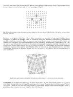
Isothermal Sections. Composition values in the triangular isothermal sections are read from a triangular grid consisting of
three sets of lines parallel to the faces and placed at regular composition intervals (see Fig. 11). Normally, the point of the
triangle is placed at the top of the illustration, component A is placed at the bottom left, B at the bottom right, and C at the
top. The amount of constituent A is normally indicated from point C to point A, the amount of constituent B from point A
to point B, and the amount of constituent C from point B to point C. This scale arrangement is often modified when only a
corner area of the diagram is shown.

Fig. 11 Triangular composition grid for isothermal sections; X is the composition of each constituent in mole fraction or percent


Projected Views. Liquidus, solidus, and solvus surfaces by their nature are not isothermal. Therefore, equal-temperature
(isothermal) contour lines are often added to the projected views of these surfaces to indicate the shape of the surfaces
(see Fig. 12). In addition to (or instead of) contour lines, views often show lines indicating the temperature troughs (also
called "valleys" or "grooves") formed at the intersections of two surfaces. Arrowheads are often added to these lines to
indicate the direction of decreasing temperature in the trough.

Fig. 12 Liquidus projection of a ternary phase diagram showing isothermal contour lines. Source: adapted from Ref 1


Reference cited in this section
1.

F.N. Rhines, Phase Diagrams in Metallurgy: Their Development and Application, McGraw-Hill, 1956

Thermodynamic Principles
The reactions between components, the phases formed in a system, and the shape of the resulting phase diagram can be
explained and understood through knowledge of the principles, laws, and terms of thermodynamics, and how they apply
to the system.
Table 2 Composition conversions
The following equations can be used to make conversions in binary systems:






The equation for converting from atomic percentages to weight percentages in higher-order systems is similar to that for binary systems,
except that an additional term is added to the denominator for each additional component. For ternary systems, for example:







The conversion from weight to atomic percentages for higher-order systems is easy to accomplish on a computer with a spreadsheet
program.

Internal Energy. The sum of the kinetic energy (energy of motion) and potential energy (stored energy) of a system is
called its internal energy, E. Internal energy is characterized solely by the state of the system.
Closed System. A thermodynamic system that undergoes no interchange of mass (material) with its surroundings is called a
closed system. A closed system, however, can interchange energy with its surroundings.
First Law. The First Law of Thermodynamics, as stated by Julius von Mayer, James Joule, and Hermann von Helmholtz in
the 1840s, says that "energy can be neither created nor destroyed." Therefore, it is called the "Law of Conservation of
Energy." This law means the total energy of an isolated system remains constant throughout any operations that are
carried out on it; that is for any quantity of energy in one form that disappears from the system, an equal quantity of
another form (or other forms) will appear.
For example, consider a closed gaseous system to which a quantity of heat energy, Q, is added and a quantity of work,
W, is extracted. The First Law describes the change in internal energy, dE, of the system as follows:
dE = Q - W


In the vast majority of industrial processes and material applications, the only work done by or on a system is limited to
pressure/volume terms. Any energy contributions from electric, magnetic, or gravitational fields are neglected, except for
electrowinning and electrorefining processes such as those used in the production of copper, aluminum, magnesium, the
alkaline metals, and the alkaline earth metals. With the neglect of field effects, the work done by a system can be
measured by summing the changes in volume, dV, times each pressure causing a change. Therefore, when field effects are
neglected, the First Law can be written:
dE = Q - PdV



Enthalpy. Thermal energy changes under constant pressure (again neglecting any field effects) are most conveniently
expressed in terms of the enthalpy, H, of a system. Enthalpy, also called heat content, is defined by:
H = E + PV


Enthalpy, like internal energy, is a function of the state of the system, as is the product PV.
Heat Capacity. The heat capacity, C, of a substance is the amount of heat required to raise its temperature one degree, that
is:


However, if the substance is kept at constant volume (dV = 0):
Q = dE


and


If, instead, the substance is kept at constant pressure (as in many metallurgical systems):


and


Second Law. While the First Law establishes the relationship between the heat absorbed and the work performed by a
system, it places no restriction on the source of the heat or its flow direction. This restriction, however, is set by the
Second Law of Thermodynamics, which was advanced by Rudolf Clausius and William Thomson (Lord Kelvin). The
Second Law says that "the spontaneous flow of heat always is from the higher temperature body to the lower temperature
body." In other words, "all naturally occurring processes tend to take place spontaneously in the direction that will lead to
equilibrium."
Entropy. The Second Law is most conveniently stated in terms entropy, S, another property of state possessed by all

systems. Entropy represents the energy (per degree of absolute temperature, T) in a system that is not available for work.
In terms of entropy, the Second Law says that "all natural processes tend to occur only with an increase in entropy, and
the direction of the process always is such as to lead to an increase in entropy." For processes taking place in a system in
equilibrium with its surroundings, the change in entropy is defined as follows:


Third Law. A principle advanced by Theodore Richards, Walter Nernst, Max Planck, and others, often called the Third
Law of Thermodynamics, states that "the entropy of all chemically homogeneous materials can be taken as zero at
absolute zero temperature" (0 K). This principle allows calculation of the absolute values of entropy of pure substances
solely from heat capacity.
Gibbs Energy. Because both S and V are difficult to control experimentally, an additional term, Gibbs energy, G,is
introduced, whereby:
G E + PV - TS H - TS


and
dG = dE + PdV + VdP - TdS - SdT


However,
dE = TdS - PdV


Therefore,
dG = VdP - SdT


Here, the change in Gibbs energy of a system undergoing a process is expressed in terms of two independent variables
pressure and absolute temperature which are readily controlled experimentally. If the process is carried out under
conditions of constant pressure and temperature, the change in Gibbs energy of a system at equilibrium with its

surroundings (a reversible process) is zero. For a spontaneous (irreversible) process, the change in Gibbs energy is less
than zero (negative); that is, the Gibbs energy decreases during the process, and it reaches a minimum at equilibrium.
Thermodynamics and Phase Diagrams
The areas (fields) in a phase diagram, and the position and shapes of the points, lines, surfaces, and intersections in it, are
controlled by thermodynamic principles and the thermodynamic properties of all of the phases that comprise the system.
Phase-Field Rule. The phase rule specifies that at constant temperature and pressure, the number of phases in adjacent
fields in a multicomponent diagram must differ by one.
Theorem of Le Châtelier. The theorem of Henri Le Châtelier, which is based on thermodynamic principles, says that "if a
system in equilibrium is subjected to a constraint by which the equilibrium is altered, a reaction occurs that opposes the
constraint, that is, a reaction that partially nullifies the alteration." The effect of this theorem on lines in a phase diagram
can be seen in Fig. 2. The slopes of the sublimation line (1) and the vaporization line (3) show that the system reacts to
increasing pressure by making the denser phases (solid and liquid) more stable at higher pressure. The slope of the
melting line (2) indicates that this hypothetical substance contracts on freezing. (Note that the boundary between liquid
water and ordinary ice, which expands on freezing, slopes towards the pressure axis.)
Clausius-Clapeyron Equation. The theorem of Le Châtelier was quantified by Benoit Clapeyron and Rudolf Clausius to give
the following equation:


where dP/dT is the slope of the univariant lines in a PT diagram such as those shown in Fig. 2, ∆V is the difference in
molar volume of the two phases in the reaction, and ∆H is difference in molar enthalpy of the two phases (the heat of the
reaction).
Solutions. The shape of liquidus, solidus, and solvus curves (or surfaces) in a phase diagram are determined by the Gibbs
energies of the relevant phases. In this instance, the Gibbs energy must include not only the energy of the constituent
components, but also the energy of mixing of these components in the phase.
Consider, for example, the situation of complete miscibility shown in Fig. 3. The two phases, solid and liquid, are in
stable equilibrium in the two-phase field between the liquidus and solidus lines. The Gibbs energies at various
temperatures are calculated as a function of composition for ideal liquid solutions and for ideal solid solutions of the two
components, A and B. The result is a series of plots similar to those in Fig. 13(a) to 13(e).

Fig. 13

Use of Gibbs energy curves to construct a binary phase diagram that shows miscibility in both the liquid and solid states. Source:
adapted from Ref 2
At temperature T
1
, the liquid solution has the lower Gibbs energy and, therefore, is the more stable phase. At T
2
, the
melting temperature of A, the liquid and solid are equally stable only at a composition of pure A. At temperature T
3
,
between the melting temperatures of A and B, the Gibbs energy curves cross. Temperature T
4
is the melting temperature
of B, while T
5
is below it.
Construction of the two-phase liquid-plus-solid field of the phase diagram in Fig. 13(f) is as follows. According to
thermodynamic principles, the compositions of the two phases in equilibrium with each other at temperature T
3
can be
determined by constructing a straight line that is tangential to both curves in Fig. 13(c). The points of tangency, 1 and 2,
are then transferred to the phase diagram as points on the solidus and liquidus, respectively. This is repeated at sufficient
temperatures to determine the curves accurately.
If, at some temperature, the Gibbs energy curves for the liquid and the solid tangentially touch at some point, the resulting
phase diagram will be similar to those shown in Fig. 4(a) and 4(b), where a maximum or minimum appears in the liquidus
and solidus curves.
Mixtures. The two-phase field in Fig. 13(f) consists of a mixture of liquid and solid phases. As stated above, the
compositions of the two phases in equilibrium at temperature T
3
are C

1
and C
2
. The horizontal isothermal line connecting
points 1 and 2, where these compositions intersect temperature T
3
, is called a tie line. Similar tie lines connect the
coexisting phases throughout all two-phase fields (areas) in binary and (volumes) in ternary systems, while tie triangles
connect the coexisting phases throughout all three-phase regions (volumes) in ternary systems.
Eutectic phase diagrams, a feature of which is a field where there is a mixture of two solid phases, also can be constructed
from Gibbs energy curves. Consider the temperatures indicated on the phase diagram in Fig. 14(f) and the Gibbs energy
curves for these temperatures (Fig. 14a to 14e). When the points of tangency on the energy curves are transferred to the
diagram, the typical shape of a eutectic system results. The mixture of solid α and β that forms upon cooling through the
eutectic point 10 has a special microstructure, as discussed later.

Fig. 14 Use of Gibbs energy curves to construct a binary phase diagram of the eutectic type. Source: adapted from Ref 3
Binary phase diagrams that have three-phase reactions other than the eutectic reaction, as well as diagrams with multiple
three-phase reactions, also can be constructed from appropriate Gibbs energy curves. Likewise, Gibbs energy surfaces
and tangential planes can be used to construct ternary phase diagrams.
Curves and Intersections. Thermodynamic principles also limit the shape of the various boundary curves (or surfaces) and
their intersections. For example, see the PT diagram shown in Fig. 2. The Clausius-Clapeyron equation requires that at the
intersection of the triple curves in such a diagram, the angle between adjacent curves should never exceed 180°, or
alternatively, the extension of each triple curve between two phases must lie within the field of third phase.
The angle at which the boundaries of two-phase fields meet also is limited by thermodynamics. That is, the angle must be
such that the extension of each beyond the point of intersection projects into a two-phase field, rather than a one-phase
field. An example of correct intersections can be seen in Fig. 6(b), where both the solidus and solvus lines are concave.
However, the curvature of both boundaries need not be concave.
Congruent Transformations. The congruent point on a phase diagram is where different phases of same composition are in
equilibrium. The Gibbs-Konovalov Rule for congruent points, which was developed by Dmitry Konovalov from a
thermodynamic expression given by J. Willard Gibbs, states that the slope of phase boundaries at congruent

transformations must be zero (horizontal). Examples of correct slope at the maximum and minimum points on liquidus
and solidus curves can be seen in Fig. 4.
Higher-Order Transitions. The transitions considered in this article up to now have been limited to the common
thermodynamic types called first-order transitions, that is, changes involving distinct phases having different lattice
parameters, enthalpies, entropies, densities, and so forth. Transitions not involving discontinuities in composition,
enthalpy, entropy, or molar volume are called higher-order transitions and occur less frequently. The change in the
magnetic quality of iron from ferromagnetic to paramagnetic as the temperature is raised above 771 °C (1420 °F) is an
example of a second-order transition: no phase change is involved and the Gibbs phase rule does not come into play in the
transition.
Another example of a higher-order transition is the continuous change from a random arrangement of the various kinds of
atoms in a multicomponent crystal structure (a disordered structure) to an arrangement where there is some degree of
crystal ordering of the atoms (an ordered structure, or superlattice), or the reverse reaction.

References cited in this section
2.

A. Prince, Alloy Phase Equilibria, Elsevier, 1966
3.

P. Gordon, Principles of Phase Diagrams in Materials Systems, McGraw-
Hill, 1968; reprinted by Robert E.
Krieger Publishing, 1983

Reading Phase Diagrams
Composition Scales. Phase diagrams to be used by scientists are usually plotted in atomic percentage (or mole
fraction), while those to be used by engineers are usually plotted in weight percentage. Conversions between weight and
atomic composition also can be made using the equations given in Table 2 and standard atomic weights listed in the
periodic table (the periodic table and atomic weights of the elements can be found in the article entitled "The Chemical
Elements" in this Section).
Lines and Labels. Magnetic transitions (Curie temperature and Néel temperature) and uncertain or speculative

boundaries are usually shown in phase diagrams as nonsolid lines of various types.
The components of metallic systems, which usually are pure elements, are identified in phase diagrams by their symbols.
Allotropes of polymorphic elements are distinguished by small (lower-case) Greek letter prefixes.
Terminal solid phases are normally designated by the symbol (in parentheses) for the allotrope of the component element,
such as (Cr) or (αTi). Continuous solid solutions are designated by the names of both elements, such as (Cu,Pd) or (βTi,
βY).
Intermediate phases in phase diagrams are normally labeled with small (lower-case) Greek letters. However, certain
Greek letters are conventionally used for certain phases, particularly disordered solutions: for example, βfor disordered
body-centered cubic (bcc), or ε for disordered close-packed hexagonal (cph), γ for the γ-brass-type structure, and σ for
the σCrFe-type structure.
For line compounds, a stoichiometric phase name is used in preference to a Greek letter (for example, A
2
B
3
rather than δ).
Greek letter prefixes are used to indicate high- and low-temperature forms of the compound (for example, αA
2
B
3
for the
low-temperature form and βA
2
B
3
for the high-temperature form).
Lever Rule. As explained in the section on "Thermodynamics and Phase Diagrams," a tie line is an imaginary horizontal
line drawn in a two-phase field connecting two points that represent two coexisting phases in equilibrium at the
temperature indicated by the line. Tie lines can be used to determine the fractional amounts of the phases in equilibrium
by employing the lever rule. The lever rule is a mathematical expression derived by the principle of conservation of
matter in which the phase amounts can be calculated from the bulk composition of the alloy and compositions of the

conjugate phases, as shown in Fig. 15(a).

Fig. 15 Portion of a binary phase diagram containing a two-phase liquid-plus-solid field illustrating
(a)
application of the lever rule to (b) equilibrium freezing, (c) nonequilibrium freezing, and (d) heating of a
homogenized sample. Source: Ref 1
At the left end of the line between α
1
and L
1
, the bulk composition is Y% component B and 100 - Y% component A, and
consists of 100% α solid solution. As the percentage of component B in the bulk composition moves to the right, some
liquid appears along with the solid. With further increases in the amount of B in the alloy, more of the mixture consists of
liquid, until the material becomes entirely liquid at the right end of the tie line. At bulk composition X, which is less than
halfway to point L
1
, there is more solid present than liquid. The lever rule says that the percentages of the two phases
present can be calculated as follows:


It should be remembered that the calculated amounts of the phases present are either in weight or atomic percentages, and
as shown in Table 3, do not directly indicate the area or volume percentages of the phases observed in microstructures.
Table 3 Volume fraction
In order to relate the weight fraction of a phase present in an alloy specimen as determined from a phase diagram to its two-dimensional
appearance as observed in a micrograph, it is necessary to be able to convert between weight-fraction values and area-fracture values,
both in decimal fractions. This conversion can be developed as follows:
The weight fraction of the phase is determined from the phase diagram, using the lever rule.
Volume portion of the phase = (Weight fraction of the phase)/(Phase density)
Total volume of all phases present = Sum of the volume portions of each phase.
Volume fraction of the phase = (Weight fraction of the phase)/(Phase density × total volume)

It has been shown by stereology and quantitative metallography that areal fraction is equal to volume fraction (Ref 6). (Areal fraction of a
phase is the sum of areas of the phase intercepted by a microscopic traverse of the observed region of the specimen divided by the total
area of the observed region.) Therefore:
Areal fraction of the phase = (Weight fraction of the phase)/(Phase density × total volume)
The phase density value for the preceding equation can be obtained by measurements or calculation. The densities of chemical elements,
and some line compounds, can be found in the literature. Alternatively, the density of a unit cell of a phase comprising one or more
elements can be calculated from information about its crystal structure and the atomic weights of the elements comprising it as follows:
Total cell weight = Sum of weights of each element
Density = Total cell weight/cell volume
For example, the calculated density of pure copper, which has a fcc structure and a lattice parameter of 0.36146 nm, is:



Phase-Fraction Lines. Reading the phase relationships in many ternary diagram sections (and other types of sections)
often can be difficult due to the great many lines and areas present. Phase-fraction lines are used by some to simplify this
task. In this approach, the sets of often nonparallel tie lines in the two-phase fields of isothermal sections (see Fig. 16a)
are replaced with sets of curving lines of equal phase fraction (Fig. 16b). Note that the phase-fraction lines extend through
the three-phase region where they appear as a triangular network. As with tie lines, the number of phase-fraction lines
used is up to the individual using the diagram. While this approach to reading diagrams may not seem helpful for such a
simple diagram, it can be a useful aid in more complicated systems. For more information on this topic, see Ref 4 and 5.

Fig. 16 Alternative systems for showing phase relationships in multiphase regions of ternary-
diagram
isothermal sections. (a) Tie lines. (b) Phase-fraction lines. Source: Ref 4
Solidification. Tie lines and the lever rule can be used to understand the freezing of a solid-solution alloy. Consider the
series of tie lines at different temperature shown in Fig. 15(b), all of which intersect the bulk composition X. The first
crystals to freeze have the composition α
1
. As the temperature is reduced to T
2

and the solid crystals grow, more A atoms
are removed from the liquid than B atoms, thus shifting the composition of the remaining liquid to composition L
2
.
Therefore, during freezing, the compositions of both the layer of solid freezing out on the crystals and the remaining
liquid continuously shift to higher B contents and become leaner in A. Therefore, for equilibrium to be maintained, the
solid crystals must absorb B atoms from the liquid and B atoms must migrate (diffuse) from the previously frozen
material into subsequently deposited layers. When this happens, the average composition of the solid material follows the
solidus line to temperature T
4
where it equals the bulk composition of the alloy.
Coring. If cooling takes place too rapidly for maintenance of equilibrium, the successive layers deposited on the crystals
will have a range of local compositions from their centers to their edges (a condition known as coring). Development of
this condition is illustrated in Fig. 15(c). Without diffusion of B atoms from the material that solidified at temperature T
1

into the material freezing at T
2
, the average composition of the solid formed up to that point will not follow the solidus
line. Instead it will remain to the left of the solidus, following compositions α'
1
through α'
3
. Note that final freezing does
not occur until temperature T
5
, which means that nonequilibrium solidification takes place over a greater temperature
range than equilibrium freezing. Because most metals freeze by the formation and growth of "treelike" crystals, called
dendrites, coring is sometimes called dendritic segregation. An example of cored dendrites is shown in Fig. 17.


Fig. 17 Copper alloy 71500 (Cu-30Ni) ingot. Dendritic structure shows coring: light areas are nickel-rich;
dark
areas are low in nickel. 20×. Source: Ref 6
Liquation. Because the lowest freezing material in a cored microstructure is segregated to the edges of the solidifying
crystals (the grain boundaries), this material can remelt when the alloy sample is heated to temperatures below the
equilibrium solidus line. If grain-boundary melting (called liquation or "burning") occurs while the sample also is under
stress, such as during hot forming, the liquefied grain boundaries will rupture and the sample will lose its ductility and be
characterized as hot short.
Liquation also can have a deleterious effect on the mechanical properties (and microstructure) of the sample after it
returns to room temperature. This is illustrated in Fig. 15(d) for a homogenized sample. If homogenized alloy X is heated
into the liquid-plus-solid region for some reason (inadvertently or during welding, etc.), it will begin to melt when it
reaches temperature T
2
; the first liquid to appear will have the composition L
2
. When the sample is heated at normal rates
to temperature T
1
, the liquid formed so far will have a composition L
1
, but the solid will not have time to reach the
equilibrium composition α
1
. The average composition will instead lie at some intermediate value such as α'
1
. According to
the lever rule, this means that less than the equilibrium amount of liquid will form at this temperature. If the sample is
then rapidly cooled from temperature T
1
, solidification will occur in the normal manner, with a layer of material having

composition α
1
deposited on existing solid grains. This is followed by layers of increasing B content up to composition α
3

at temperature T
3
, where all of the liquid is converted to solid. This produces coring in the previously melted regions
along the grain boundaries and sometimes even voids that decrease the strength of the sample. Homogenization heat
treatment will eliminate the coring, but not the voids.
Eutectic Microstructures. When an alloy of eutectic composition is cooled from the liquid state, the eutectic reaction
occurs at the eutectic temperature, where the two distinct liquidus curves meet. At this temperature, both α and β solid
phases must deposit on the grain nuclei until all of the liquid is converted to solid. This simultaneous deposition results in
microstructures made up of distinctively shaped particles of one phase in a matrix of the other phase, or alternate layers of
the two phases. Examples of characteristic eutectic microstructures include spheroidal, nodular, or globular; acicular
(needles) or rod; and lamellar (platelets, Chinese script or dendritic, or filigreed). Each eutectic alloy has its own
characteristic microstructure, when slowly cooled (see Fig. 18). Cooling more rapidly, however, can affect the
microstructure obtained (see Fig. 19). Care must be taken in characterizing eutectic structures because elongated particles
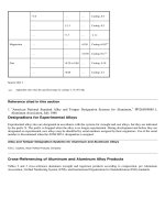
can appear nodular and flat platelets can appear elongated or needlelike when viewed in cross section.

Fig. 18 Examples of characteristic eutectic microstructures in slowly cooled alloys. (a) 40Sn-
50In alloy showing
globules of tin-rich intermetallic phase (light) in a matrix of dark indium-rich intermetallic phase. 150×. (b) Al-
13Si alloy showing an acicular structure consisting of short, a
ngular particles of silicon (dark) in a matrix of
aluminum. 200×. (c) Al-33Cu alloy showing a lamellar structure consisting of dark platelets of CuAl
2
and light
platelets of aluminum solid solution. 180×. (d) Mg-37Sn alloy showing a lamellar structure consisting of Mg
2

Sn
"Chinese-script" (dark) in a matrix of magnesium solid solution. 250×. Source: Ref 6

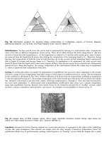
Fig. 19 Effect of cooling rate on the microstructure of Sn-
37Pb alloy (eutectic soft solder). (a) Slowly cooled
sample shows a lamellar structure consisting of dark platelets of lead-
rich solid solution and light platelets of
tin. 375×. (b) More rapidly cooled sample shows globules of lead-
rich solid solution, some of which exhibit a
slightly dendritic structure, in a matrix of tin. 375×. Source: Ref 6
If the alloy has a composition different than the eutectic composition, the alloy will begin to solidify before the eutectic
temperature is reached. If the alloy is hypoeutectic, some dendrites of will form in the liquid before the remaining liquid
solidifies at the eutectic temperature. If the alloy is hypereutectic, the first (primary) material to solidify will be dendrites
of . The microstructure produced by slow cooling of a hypoeutectic and hypereutectic alloy will consist of relatively
large particles of primary constituent, consisting of the phase that begins to freeze first surrounded by relatively fine
eutectic structure. In many instances, the shape of the particles will show a relationship to their dendritic origin (see Fig.
20a). In other instances, the initial dendrites will have filled out somewhat into idiomorphic particles (particles having
their own characteristic shape) that reflect the crystal structure of the phase (see Fig. 20b).

Fig. 20 Examples of primary-particle shape. (a) Sn-30Pb hypoeutectic alloy showing dendritic particles of tin-
rich solid solution in a matrix of tin-lead eutectic. 500×. (b) Al-19Si hypereutectic alloy, phosphorus-
modified,
showing idiomorphic particles of silicon in a matrix of aluminum-silicon eutectic. 100×. Source: Ref 6
As stated earlier, cooling at a rate that does not allow sufficient time to reach equilibrium conditions will affect the
resulting microstructure. For example, it is possible for an alloy in a eutectic system to obtain some eutectic structure in
an alloy outside the normal composition range for such a structure. This is illustrated in Fig. 21. With relatively rapid
cooling of alloy X, the composition of the solid material that forms will follow line
1
- '
4

rather than solidus line to
4
.
As a result, the last liquid to solidify will have the eutectic composition L
4
rather than L
3
, and will form some eutectic
structure in the microstructure. The question of what takes place when the temperature reaches T
5
is discussed later.

Fig. 21
Binary phase diagram, illustrating the effect of cooling rate on an alloy lying outside the equilibrium
eutectic-
transformation line. Rapid solidification into a terminal phase field can result in some eutectic structure
being formed; homogenization at temperatures in the single-phase field will eliminate the eutectic structure;
phase will precipitate out of solution upon slow cooling into the -plus- field. Source: adapted from Ref 1
Eutectoid Microstructures. Because the diffusion rates of atoms are so much lower in solids than liquids,
nonequilibrium transformation is even more important in solid/solid reactions (such as the eutectoid reaction) than in
liquid/solid reactions (such as the eutectic reaction). With slow cooling through the eutectoid temperature, most alloys of
eutectoid composition such as alloy 2 in Fig. 22 transform from a single-phase microstructure to a lamellar structure
consisting of alternate platelets of and arranged in groups (or "colonies"). The appearance of this structure is very
similar to lamellar eutectic structure (see Fig. 23). When found in cast irons and steels, this structure is called "pearlite"
because of its shiny mother-of-pearl-like appearance under the microscope (especially under oblique illumination); when
similar eutectoid structure is found in nonferrous alloys, it often is called "pearlite-like" or "pearlitic."

Fig. 22 Binary phase diagram of a eutectoid system. Source: adapted from Ref 1



Fig. 23 Fe-
0.8C alloy showing a typical pearlite eutectoid structure of alternate layers of light ferrite and dark
cementite. 500×. Source: Ref 6
The terms, hypoeutectoid and hypereutectoid have the same relationship to the eutectoid composition as hypoeutectic and
hypereutectic do in a eutectic system; alloy 1 in Fig. 22 is a hypoeutectoid alloy, while alloy 3 is hypereutectoid. The
solid-state transformation of such alloys takes place in two steps, much like freezing of hypoeutectic and hypereutectic
alloys except that the microconstituents that form before the eutectoid temperature is reached are referred to as
proeutectoid constituents rather than "primary."
Microstructures of Other Invariant Reactions. Phase diagrams can be used in a manner similar to that used in the
discussion of eutectic and eutectoid reactions to determine the microstructures expected to result from cooling an alloy
through any of the other six types of reactions listed in Table 1.
Solid-State Precipitation. If alloy X in Fig. 21 is homogenized at a temperature between T
3
and T
5
, it will reach
equilibrium condition; that is, the portion of the eutectic constituent will dissolve and the microstructure will consist
solely of grains. Upon cooling below temperature T
5
, this microstructure will no longer represent equilibrium
conditions, but instead will be supersaturated with B atoms. In order for the sample to return to equilibrium, some of the