Practical Design Calculations for Groundwater and Soil Remediation - Chapter 6 docx
Bạn đang xem bản rút gọn của tài liệu. Xem và tải ngay bản đầy đủ của tài liệu tại đây (519.62 KB, 47 trang )
Kuo, Jeff "Groundwater remediation"
Practical Design Calculations for Groundwater and Soil Remediation
Boca Raton: CRC Press LLC,1999
chapter six
Groundwater remediation
This chapter starts with design calculations for capture zone and optimal
well spacing. The rest of the chapter focuses on design calculations for
commonly used in situ and ex situ groundwater remediation techniques,
including bioremediation, air sparging, air stripping, advanced oxidation
processes, and activated carbon adsorption.
VI.1
Hydraulic control (groundwater extraction)
When a groundwater aquifer is contaminated, groundwater extraction is
often needed. Groundwater extraction through pumping mainly serves two
purposes: (1) to minimize the plume migration or spreading and (2) to reduce
the contaminant concentrations in the impacted aquifer. The extracted water
often needs to be treated before being injected back into the aquifer or
released to surface water bodies. Pump and treat is a general term used for
groundwater remediation that removes contaminated groundwater and
treats it above ground.
Groundwater extraction is typically accomplished through one or more
pumping or extraction wells. Pumping of groundwater stresses the aquifer
and creates a cone of depression or a capture zone. Choosing appropriate
locations for the pumping wells and spacing among the wells is an important
component in design. Pumping wells should be strategically located to
accomplish rapid mass removal from areas of the groundwater plume where
contaminants are heavily concentrated. On the other hand, they should be
located to allow full capture of the plume to prevent further migration. In
addition, if containment is the only objective for the groundwater pumping,
the extraction rate should be established at a minimum rate sufficient to
prevent the plume migration. (The more the groundwater is extracted, the
higher the treatment cost.) On the other hand, if groundwater cleanup is
required, the extraction rate may need to be enhanced to shorten the remediation time. For both cases, major questions to be answered for design of
a groundwater pump-and-treat program are
©1999 CRC Press LLC
1.
2.
3.
4.
5.
6.
7.
What is the optimum number of pumping wells required?
Where would be the optimal locations of the extraction wells?
What would be the size (diameter) of the wells?
What would be the depth, interval, and size of the perforations?
What would be the construction materials of the wells?
What would be the optimum pumping rate for each well?
What would be the optimal treatment method for the extracted
groundwater?
8. What would be the disposal method for the treated groundwater?
This section will illustrate common design calculations to determine the
influence of a pumping well. The results from these calculations can provide
answers to some of the above questions.
VI.1.1
Cone of depression
When a groundwater extraction well is pumped, the water level in its vicinity
will decline to provide a gradient to drive water toward the well. The
gradient is steeper as the well is approached, and this results in a cone of
depression. In dealing with groundwater contamination problems, evaluation of the cone of depression of a pumping well is critical because it represents the limit that the well can reach.
The equations describing the steady-state flow of an aquifer from a fully
penetrating well have been discussed earlier in Section III.2. The equations
were used in that section to estimate the drawdown in the wells as well as
the hydraulic conductivity of the aquifer. These equations can also be used
to estimate the radius of influence of a groundwater extraction well or to
estimate the groundwater pumping rate. This section will illustrate these
applications.
Steady-state flow in a confined aquifer
The equation describing steady-state flow of a confined aquifer (an artesian
aquifer) from a fully penetrating well is shown below. A fully penetrating
well means that the groundwater can enter at any level from the top to the
bottom of the aquifer.
Q=
Kb( h2 − h1 )
for American Practical Units
528 log(r2 / r1 )
2.73 Kb( h2 − h1 )
=
for SI
log(r2 / r1 )
[Eq. VI.1.1]
where Q = pumping rate or well yield (in gpm or m3/d), h1, h2 = static head
measured from the aquifer bottom (in ft or m), r1, r2 = radial distance from
©1999 CRC Press LLC
the pumping well (in ft or m), b = thickness of the aquifer (in ft or m), and
K = hydraulic conductivity of the aquifer (in gpd/ft2 or m/d).
Example VI.1.1A
Radius of influence from pumping a confined
aquifer
A confined aquifer 30 ft (9.1 m) thick has a piezometric surface 80 ft (24.4
m) above the bottom confining layer. Groundwater is being extracted from
a 4-in (0.1 m) diameter fully penetrating well.
The pumping rate is 40 gpm (0.15 m3/min). The aquifer is relatively
sandy with a hydraulic conductivity of 200 gpd/ft2. Steady-state drawdown
of 5 ft (1.5 m) is observed in a monitoring well 10 ft (3.0 m) from the pumping
well. Determine
a. The drawdown in the pumping well
b. The radius of influence of the pumping well
Solutions:
a. First let us determine h1 (at r1 = 10 ft):
h1 = 80 – 5 = 75 ft
(or = 24.4 – 1.5 = 22.9 m)
To determine the drawdown at the pumping well, set r at the well =
well radius = (2/12) ft = 0.051 m and use Eq. VI.1.1:
40 =
(200)(30)( h2 − 75)
→ h2 = 68.7 ft
528 log[(2 / 12)/ 10]
or
[(0.15)(1440)] =
2.73[(200)(0.0410)](9.1)( h2 − 22.9)
→ h2 = 21.0 m
log(0.051/ 3.0)
So, the drawdown in the pumping well = 80 – 68.7 = 11.3 ft (or = 24.4
– 21.0 = 3.4 m).
b. To determine the radius of influence of the pumping well, set r at the
radius of influence (rRI) to be the location where the drawdown is
equal to zero. We can use the drawdown information of the pumping
well as
40 =
or
©1999 CRC Press LLC
(200)(30)(68.7 − 80)
→ rRI = 270 ft
528 log[(2 / 12)/ rRI ]
[(0.15)(1440)] =
2.73[(200)(0.0410)](9.1)(21.0 - 24.4)
→ rRI = 82 m
log(0.051/ rRI )
Similar results can also be derived from using the drawdown information of the observation well as
40 =
(200)(30)(75 − 80)
→ rRI = 263 ft
528 log[10 / rRI ]
or
[(0.15)(1440)] =
2.73[(200)(0.0410)](9.1)(22.9 − 24.4)
→ h2 = 78 m
log(3/rRI )
Discussion
1. In (a), 0.041 is the conversion factor to convert the hydraulic conductivity from gpd/ft2 to m/day. The factor was taken from Table III.1.A.
2. Calculations in (a) have demonstrated that the results would be the
same by using two different systems of units.
3. The “h1 – h2” term can be replaced by “s2 – s1,” where s1 and s2 are the
drawdown values at r1 and r2, respectively.
4. The differences in the calculated rRI values in (b) come mainly from
the unit conversions and data truncations.
Example VI.1.1B
Estimate the groundwater extraction rate
of a confined aquifer from steady-state
drawdown data
Use the following information to estimate the groundwater extraction rate
of a pumping well in a confined aquifer:
Aquifer thickness = 30.0 ft (9.1 m) thick
Well diameter = 4-in (0.1 m) diameter
Well perforation depth = full penetrating
Hydraulic conductivity of the aquifer = 400 gpd/ft2
Steady-state drawdown = 2.0 ft observed in a monitoring well 5 ft from
the pumping well = 1.2 ft observed in a monitoring well 20 ft from
the pumping well
Solutions:
Inserting the data into Eq. VI.1.1, we obtain
Q=
Kb( h2 − h1 )
( 400)(30)(2.0 − 1.2)
=
= 30.2 gpm
528 log(r2 / r1 )
528 log(20 / 5)
©1999 CRC Press LLC
Discussion. The “h1 – h2” term can be replaced by “s2 – s1,” where s1
and s2 are the drawdown values at r1 and r2, respectively.
Example VI.1.1C
Estimate the pumping rate from a confined
aquifer
Determine the rate of discharge (in gpm) of a confined aquifer being pumped
by a fully penetrating well. The aquifer is composed of medium sand. It is
90 ft thick with a hydraulic conductivity of 550 gpd/ft2. The drawdown of
an observation well 50 ft away is 10 ft, and the drawdown in a second
observation well 500 ft away is 1 ft.
Solution:
This problem is very similar to Ex. VI.1.1B. The flow rate can be calculated
by using Eq. VI.1.1 as
Q=
=
Kb( h2 − h1 )
Kb( H − h)
=
528 log( R / r ) 528 log(r2 / r1 )
(550)(90)[(90 − 1) − (90 − 10)]
= 844 gpm
(528) log(500 / 50)
Steady-state flow in an unconfined aquifer
The equation describing the steady-state flow of an unconfined aquifer
(water-table aquifer) from a fully penetrating well can be expressed as
Q=
2
2
K( h2 − h1 )
1055 log(r2 / r1 )
2
2
1.366 K( h2 − h1 )
=
log(r2 / r1 )
for American Practical Units
[Eq. VI.1.2]
for SI
All the terms are as defined for Eq. VI.1.1.
Example VI.1.1D
Radius of influence from pumping an unconfined
aquifer
A water-table aquifer is 40 ft (12.2 m) thick. Groundwater is being extracted
from a 4-inch (0.1 m) diameter fully penetrating well.
The pumping rate is 40 gpm (0.15 m3/min). The aquifer is relatively
sandy with a hydraulic conductivity of 200 gpd/ft2. Steady-state drawdown
of 5 ft (1.5 m) is observed in a monitoring well at 10 ft (3.0 m) from the
pumping well. Estimate
©1999 CRC Press LLC
a. The drawdown in the pumping well
b. The radius of influence of the pumping well
Solutions:
a. First let us determine h1 (at r1 = 10 ft):
h1 = 40 – 5 = 35 ft
(or = 12.2 – 1.5 = 10.7 m)
To determine the drawdown at the pumping well, set r at the well =
well radius = (2/12) ft = 0.051 m, and use Eq. VI.1.2:
40 =
2
(200)( h2 − 35 2 )
→ h2 = 29.2 ft
1055 log[(2 / 12)/ 10]
or
[(0.15)(1440)] =
2
1.366[(200)(0.0410)](h2 − 10.7 2 )
→ h2 = 9.0 m
log(0.051/ 3.0)
So, the drawdown in the extraction well = 40 – 29.2 = 10.8 ft (or =
12.2 – 9.0 = 3.2 m).
b. To determine the radius of influence of the pumping well, set r at the
radius of influence (rRI) to be the location where the drawdown is
equal to zero. We can use the drawdown information of the pumping
well as
40 =
(200)(29.2 2 − 40 2 )
→ rRI = 580 ft
1055 log[(2 / 12)/ rRI ]
or
[(0.15)(1440)] =
1.366[(200)(0.0410)](9.0 2 − 12.2 2 )
→ rRI = 168 m
log(0.051/ rRI )
Similar results can also be derived from using the drawdown information of the observation well as
40 =
or
©1999 CRC Press LLC
(200)(35 2 − 40 2 )
→ rRI = 598 ft
1055 log[10 / rRI ]
[(0.15)(1440)] =
1.366[(200)(0.0410)](10.7 2 − 12.2 2 )
→ rRI = 181 m
log(3 / rRI )
Discussion
1. In Eq. VI.1. for confined aquifers, the “h1 – h2” term can be replaced
by “s2 – s1,” where s1 and s2 are the drawdown values at r1 and r2,
respectively. However, no analogy can be made here, that is, “h22 – h12”
in Eq. VI.1.2 cannot be replaced by “s12 – s22.”
2. The differences in the calculated rRI values in (b) come mainly from
the unit conversions and data truncations.
Example VI.1.1E
Estimate the groundwater extraction rate
of an unconfined aquifer from steady-state
drawdown data
Use the following information to estimate the groundwater extraction rate
of a pumping well in an unconfined aquifer:
Aquifer thickness = 30.0 ft (9.1 m) thick
Well diameter = 4-in (0.1 m) diameter
Well perforation depth = full penetrating
Hydraulic conductivity of the aquifer = 400 gpd/ft2
Steady-state drawdown = 2.0 ft observed in a monitoring well 5 ft from
the pumping well = 1.2 ft observed in a monitoring well 20 ft from
the pumping well
Solutions:
a. First we need to determine h1 and h2:
h1 = 30.0 – 2.0 = 28.0 ft
h2 = 30.0 – 1.2 = 28.8 ft
b. Inserting the data into Eq. VI.1.2, we obtain
Q=
VI.1.2
2
2
K( h2 − h1 )
400(28.8 2 − 28.0 2 )
=
= 28.6 gpm
1055 log(r2 / r1 )
1055 log(20 / 5)
Capture zone analysis
One key element in design of a groundwater extraction system is selection
of proper locations for the pumping wells. If only one well is used, the well
©1999 CRC Press LLC
should be strategically located to create a capture zone that encloses the
entire contaminant plume. If two or more wells are used, the general interest
is to find the maximum distance between any two wells such that no contaminants can escape through the interval between the wells. Once such
distances are determined, one can depict the capture zone of these wells
from the rest of the aquifer.
To delineate the capture zone of a groundwater pumping system in an
actual aquifer can be a very complicated task. To allow for a theoretical
approach, let us consider a homogeneous and isotropic aquifer with a uniform thickness and assume the groundwater flow is uniform and steady.
The theoretical treatment of this subject starts from one single well and
expands to multiple wells. The discussions are mainly based on the work
by Javandel and Tsang.2
One groundwater extraction well
For easier presentation, let the extraction well be located at the origin of an
x-y coordinate system (Figure VI.1.A). The equation of the dividing streamlines that separate the capture zone of this well from the rest of the aquifer
(sometimes referred to as the “envelope”) is
y=±
y
Q
Q
−
tan −1
x
2Bu 2 πBu
[Eq. VI.1.3]
where B = aquifer thickness (ft or m), Q = groundwater extraction rate (ft3/s
or m3/s), and u = regional groundwater velocity (ft/s or m/s) = Ki.
Figure VI.1.A illustrates the capture zone of a single pumping well. The
larger the Q/Bu value is (i.e., larger groundwater extraction rate, slower
groundwater velocity, or shallower aquifer thickness), the larger the capture
zone. Three interesting sets of x and y values of the capture zone:
Figure VI.1.A
Capture zone of a single well.
©1999 CRC Press LLC
1. The stagnation point, where y is approaching zero,
2. The sidestream distance at the line of the extraction well, where x =
0, and
3. The asymptotic values of y, where x = ∞.
If these three sets of data are determined, the rough shape of the capture
zone can be depicted. At the stagnation point (where y is approaching zero),
the distance between the stagnation point and the pumping well is equal to
Q/2πBu, which represents the farthest downstream distance that the pumping well can reach. At x = 0, the maximum sidestream distance from the
extraction well is equal to ±Q/4Bu. In other words, the distance between the
dividing streamlines at the line of the well is equal to Q/2Bu. The asymptotic
value of y (where x = ∞) is equal to ±Q/2Bu. Thus, the distance between the
streamlines far upstream from the pumping well is Q/Bu.
Note that the parameter in Eq. VI.1.3 (Q/Bu) has a dimension of length.
To draw the envelope of the capture zone, Eq. VI.1.3 can be rearranged as
x=
x=
y
2Bu
tan +1 −
yπ
Q
y
2Bu
tan −1 −
yπ
Q
for positive y values [Eq. VI.1.4A]
for negative y values [Eq. VI.1.4B]
A set of (x, y) values can be obtained from these equations by first
specifying a value of y. The envelope is symmetrical about the x-axis.
Example VI.1.2A
Draw the envelope of a capture zone of a
groundwater pumping well
Delineate the capture zone of a groundwater recovery well with the following information:
Q = 60 gpm
Hydraulic conductivity = 2000 gpd/ft2
Groundwater gradient = 0.01
Aquifer thickness = 50 ft
Solution:
a. Determine the groundwater velocity, u:
©1999 CRC Press LLC
u = (K)(i) = [(2000 gal/d/ft2)(1 d/1440 min)(1 ft3/7.48 gal)](0.01)
= 1.86 × 10⁻³ ft/min
b. Determine the value of the parameter, Q/Bu:
Q (60 gal/min)(1ft 3/7.48 gal)
=
Bu
(50 ft)(1.8 × 10 −3 ft/min)
or
=
60 gal/min
= 86.4 ft
(50 ft)[2000 gal/d/ft 2 )(1 d/1440 min)(0.01)]
c. Establish a set of the (x, y) values using Eq. VI.1.4. First specify values
of y. Select smaller intervals for small y values. The following figure
lists some of the data points used to plot Figure E.VI.1.2A.
y (ft)
x (ft)
0
0.1
1
5
10
20
30
40
0.00
–13.74
–13.73
–13.14
–11.24
–2.34
21.01
168.78
–0.1
–1
–5
–10
–20
–30
–40
–13.74
–13.73
–13.14
–11.24
–2.34
21.01
168.78
Discussion
1. The capture zone curve is symmetrical about the x-axis as shown in
the table or in the figure. Note that Eq. VI.1.4A should be used for
positive y values and Eq. VI.1.4B for negative y values.
2. Do not specify the y values beyond the values of ±Q/2Bu. As discussed, ±Q/2Bu are the asymptotic values of the capture zone curve
(x = ∞).
©1999 CRC Press LLC
Figure E.VI.1.2A
Capture zone of a single well.
Example VI.1.2B
Determine the downstream and sidestream
distances of a capture zone
A groundwater extraction well is installed in an aquifer (hydraulic conductivity = 1000 gpd/ft2, gradient = 0.015, and aquifer thickness = 80 ft).
The design pumping rate is 50 gpm. Delineate the capture zone of this
recovery well by specifying the following characteristic distances of the
capture zone:
a. The sidestream distance from the well to the envelope of the capture
zone at the line of the pumping well
b. The downstream distance from the well to the stagnation point of the
envelope
c. The sidestream distance of the envelope far upstream of the pumping
well
Solution:
a. Determine the groundwater velocity, u:
u = (K)(i) = [(1000 gal/d/ft2)(1 d/1440 min)(1 ft3/7.48 gal)](0.015)
= 1.39 × 10⁻³ ft/min
b. Determine the sidestream distance from the well to the envelope of
the capture zone at the line of the pumping well, Q/4Bu:
(50 gal/min)(1ft 3/7.48 gal)
Q
=
= 15.0 ft
4 Bu (4)(80 ft)(1.39 × 10 −3 ft/min)
c. Determine the downstream distance from the well to the stagnation
point of the envelope, Q/2πBu:
©1999 CRC Press LLC
(50 gal/min)(1ft 3/7.48 gal)
Q
=
= 9.6 ft
2πBu (2)(π)(80 ft)(1.39 × 10 −3 ft/min)
d. Determine the sidestream distance of the envelope far upstream of
the pumping well, Q/2Bu:
(50 gal/min)(1ft 3/7.48 gal)
Q
=
= 30.0 ft
2 Bu (2)(80 ft)(1.39 × 10 −3 ft/min)
e. The general shape of the envelope can be defined by using the above
characteristic distances:
x (ft)
y (ft)
0
–9.6
0
0
150*
150*
0
0
15
–15
30
–30
Note
Well location
Downstream distance (stagnation point)
Sidestream distance at the line of the well
Sidestream distance at the line of the well
Sidestream distance at far upstream of the well
Sidestream distance at far upstream of the well
* The sidestream distance far upstream of the well, ±30 ft, should occur
at x = ∞. A value of 150, which is ten times the sidestream distance at
the line of well, is used here as the value of x.
Figure E.VI.1.2B
Capture zone of a single well.
Multiple wells
Table V1.1.A summarizes some characteristic distances of the capture zone
for multiple groundwater monitoring wells located on a line perpendicular
to the flow direction. As shown in the table, the distance between the dividing streamlines far upstream from the pumping wells is equal to n(Q/Bu),
where n is the number of the pumping wells. This distance is twice the
distance between the streamlines at the line of the wells.
©1999 CRC Press LLC
The downstream distance for multiple wells is very similar to that of the
single pumping well, i.e., Q/2πBu.
Table VI.1.A
Characteristic Distances of the Capture Zone for
Groundwater Pumping Wells
No. of extraction
wells
Optimal distance
between each pair
of extraction wells
Distance between
the streamlines
at the line of
the wells
Distance between
the streamlines at
far upstream
from the wells
1
2
3
4
—
0.32 Q/Bu
0.40 Q/Bu
0.38 Q/Bu
0.5 Q/Bu
Q/Bu
1.5 Q/Bu
2 Q/Bu
Q/Bu
2 Q/Bu
3 Q/Bu
4 Q/Bu
Modified from Javandel, I. and Tsang, C.-F., Groundwater, 24(5), 616–625, 1986. With permission.
Example VI.1.2C
Determine the downstream and sidestream
distances of a capture zone for multiple wells
Two groundwater extraction wells are to be installed in an aquifer (hydraulic
conductivity = 1000 gpd/ft2, gradient = 0.015, and aquifer thickness = 80 ft).
The design pumping rate for each well is 50 gpm. Determine the optimal
distance between the two wells and delineate the capture zone of these
recovery wells by specifying the following characteristic distances of the
capture zone:
a. The sidestream distance from the wells to the envelope of the capture
zone at the line of the pumping wells
b. The downstream distance from the wells to stagnation points of the
envelope
c. The sidestream distance of the envelope far upstream of the pumping
wells
Solution:
a. Determine the groundwater velocity, u:
u = (K)(i) = [(1000 gal/d/ft2)(1 d/1440 min)(1 ft3/7.48 gal)](0.015)
= 1.39 × 10⁻³ ft/min
b. Determine the optimum distance between these two wells, 0.32 Q/Bu:
0.32Q (0.32)(50 gal/min)(1ft 3/7.48 gal)
=
= 19.2 ft
Bu
(80 ft)(1.39 × 10 −3 ft/min)
©1999 CRC Press LLC
The distance of each well to the origin is half of this value = 0.16 Q/Bu
= 9.6 ft.
c. Determine the sidestream distance from the well to the envelope of
the capture zone at the line of the pumping well, Q/2Bu:
(50 gal/min)(1ft 3/7.48 gal)
Q
=
= 30.0 ft
2 Bu (2)(80 ft)(1.39 × 10 −3 ft/min)
d. Determine the downstream distance from the well to the stagnation
point of the envelope, Q/2πBu:
(50 gal/min)(1ft 3/7.48 gal)
Q
=
= 9.6 ft
2 πBu (2)(π)(80 ft)(1.39 × 10 −3 ft/min)
e. Determine the sidestream distance of the envelope far upstream of
the pumping wells, Q/Bu:
Q (50 gal/min)(1ft 3/7.48 gal)
=
= 60.0 ft
Bu
(80 ft)(1.39 × 10 −3 ft/min)
f. The general shape of the envelope can be defined by using the above
characteristic distances:
x (ft)
y (ft)
Note
0
0
–9.6
0
0
300*
300*
9.6
–9.6
0
30
–30
60
–60
Location of the first well
Location of the second well
Downstream distance (stagnation point)
Sidestream distance at the line of the wells
Sidestream distance at the line of the wells
Sidestream distance far upstream of the wells
Sidestream distance far upstream of the wells
* The sidestream distance far upstream of the wells, ±60 ft, should occur
at x = ∞. A value of 300, which is ten times the sidestream distance
at the line of wells, is used as the value of x.
Discussion
1. The sidestream distance at the line of the two pumping wells is twice
that of the single well.
2. The sidestream distance far upstream of the two pumping wells is
twice that of the single well.
3. The downstream distance of the two pumping wells is the same as
that of the single pumping well. The calculated downstream distance,
©1999 CRC Press LLC
Figure E.VI.1.2C
Capture zone of two wells.
Q/2πBu, is along the x-axis. However, the affected distances directly
downstream of these two wells should be slightly greater than
Q/2πBu.
Well spacing and number of wells
As mentioned earlier, it is important to determine the number of wells and
their spacing in a groundwater remediation program. After the extent of the
plume, and the direction and velocity of the groundwater flow have been
determined, the following procedure can be used to determine the number
of wells and their locations:
Step 1: Determine the groundwater pumping rate from aquifer testing
or estimate the flow rate by using information of the aquifer
materials.
Step 2: Draw the capture zone of one groundwater well (see Example
VI.1.2A or VI.1.2B), using the same scale as the plume map.
Step 3: Superimpose the capture zone curve on the plume map. Make
sure the direction of the groundwater of the capture zone curve
matches that of the plume map.
Step 4: If the capture zone can completely encompass the extent of the
plume, one pumping well is the optimum number. The location
of the well on the capture zone curve is then copied to the plume
map. One may want to reduce the groundwater extraction rate
to have a smaller capture zone, but still sufficient to cover the
entire plume.
Step 5: If the capture zone cannot encompass the entire extent of the
plume, prepare the capture zone curves using two or more pumping wells until the capture zone can cover the entire plume. The
locations of the wells on the capture zone curve are then copied
to the plume map. (Note that the zones of influence of individual
wells may overlap. Consequently, one may not be able to pump
the same flow rate from each well in a network of wells as one
can from a single well with the same allowable drawdown.)
©1999 CRC Press LLC
Example VI.1.2D
Determine the number and locations of pumping
wells for capturing a groundwater plume
An aquifer (hydraulic conductivity = 1000 gpd/ft2, gradient = 0.015, and
aquifer thickness = 80 ft) is contaminated. The extent of the plume has been
defined and it is shown in Figure E.VI.1.2D. (Each interval on the x-axis is
40 ft and that on the y-axis is 20 ft.)
Determine the number and locations of groundwater extraction wells
for remediation. The design pumping rate of each well is 50 gpm.
Figure E.VI.1.2D
Capture zones of one and two wells.
Solution:
a. Plot the capture zone of a single well (same as Example VI.1.2B). The
triangle symbols on the figure define the capture zone of this single well.
As shown, this capture zone could not encompass the entire plume.
b. Plot the capture zone of two pumping wells (same as Example
VI.1.2C). The square symbols on the figure define the capture zone of
these two wells. As shown, this capture zone can encompass the entire
plume. Consequently, using two pumping wells is optimum. The
locations of these two pumping wells are shown as open circles in
the figure.
VI.2
VI.2.1
Above-ground groundwater treatment systems
Activated carbon adsorption
Adsorption is the process that collects soluble substances in solution onto
the surface of the adsorbent solids. Activated carbon is a universal adsorbent
that adsorbs almost all types of organic compounds. Activated carbon particles have a large specific surface area. In activated carbon adsorption, the
organics leave (or are removed from) the liquid by adsorbing onto the carbon
©1999 CRC Press LLC
surface. As the carbon bed becomes exhausted, as indicated by breakthrough
of contaminants in the effluent, the carbon must be regenerated or replaced.
Common preliminary design of an activated carbon adsorption system
includes sizing of the adsorber, determining the carbon-change (or regeneration) interval, and configuring the carbon units, when multiple carbon
adsorbers are used.
Adsorption isotherm and adsorption capacity
In general, the amount of materials adsorbed depends on the characteristics
of the solute and the activated carbon, the solute concentration, and the
temperature. An adsorption isotherm describes the equilibrium relationship
between the adsorbed solute concentration on the solid and the dissolved
solute concentration in the bulk solution at a given temperature. The adsorption capacity of a given activated carbon for a specific compound is estimated
from their isotherm data. The most commonly used adsorption models in
environmental applications are the Langmuir and Freundlich isotherms,
respectively:
q=
abC
1 + bC
q = kC n
[Eq. VI.2.1]
[Eq. VI.2.2]
where q is the adsorbed concentration (in mass of contaminant/mass of
activated carbon), C is the liquid concentration (in mass of contaminant/volume of solution), and a, b, k, and n are constants. The adsorption concentration, q, obtained from Eq. VI.2.1 or VI.2.2. is the equilibrium value (the one
in equilibrium with the liquid solute concentration). It should be considered
as the theoretical adsorption capacity for a specified liquid concentration.
The actual adsorption capacity in the field applications should be lower.
Normally, design engineers take 25 to 50% of this theoretical value as the
design adsorption capacity as a factor of safety. Therefore,
qactual = (50%)(qtheoretical )
[Eq. VI.2.3]
The maximum amount of contaminants that can be removed or held
(Mremoval) by a given amount of activated carbon can be determined as
Mremoval = (qactual )( Mcarbon )
= (qactual )[(Vcarbon )(ρb )]
[Eq. VI.2.4]
where Mcarbon is the mass, Vcarbon is the volume, and ρb is the bulk density of
activated carbon, respectively.
©1999 CRC Press LLC
The following procedure can be used to determine the adsorption capacity of an activated carbon adsorber:
Step 1: Determine the theoretical adsorption capacity by using Eq. VI.2.1
or VI.2.2.
Step 2: Determine the actual adsorption capacity by using Eq. VI.2.3.
Step 3: Determine the amount of activated carbon in the adsorber.
Step 4: Determine the maximum amount of contaminants that can be
held by the adsorber using Eq. VI.2.4.
Information needed for this calculation
• Adsorption isotherm
• Contaminant concentration of the influent liquid, Cin
• Volume of the activated carbon, Vcarbon
• Bulk density of the activated carbon, ρb
Example VI.2.1A
Determine the capacity of an activated carbon
adsorber
Dewatering to lower the groundwater level for below-ground construction
is often necessary. At a construction site, the contractor unexpectedly found
that the extracted groundwater was contaminated with 5 mg/L toluene. The
toluene concentration of the groundwater has to be reduced to below 100
ppb before discharge. To avoid further delay of the tight construction schedule, off-the-shelf 55-gal activated carbon units are proposed to treat the
groundwater.
The activated carbon vendor provided the adsorption isotherm information. It follows the Langmuir model as q(kg toluene/kg carbon) = [0.04Ce/(1
+ 0.002Ce)], where Ce is in mg/L. The vendor also provided the following
information regarding the adsorber:
Diameter of carbon packing bed in each 55-gal drum = 1.5 ft
Height of carbon packing bed in each 55-gal drum = 3 ft
Bulk density of the activated carbon = 30 lb/ft3
Determine (a) the adsorption capacity of the activated carbon, (b) the
amount of activated carbon in each 55-gal unit, and (c) the amount of the
toluene that each unit can remove before exhausted.
Solution:
a. The theoretical adsorption capacity can be found by using Eq. VI.2.1 as
q(kg/kg) =
©1999 CRC Press LLC
0.004Ce
(0.004)(5)
=
= 0.02 kg/kg
1 + 0.002Ce 1 + (0.002)(5)
The actual adsorption capacity can be found by using Eq. VI.2.3 as
qactual = (50%)qtheoretical = (50%)(0.02) = 0.01 kg/kg
b. Volume of the activated carbon inside a 55-gal drum = (πr2)(h)
= (π)[(1.5/2)2](3) = 5.3 ft3
Amount of the activated carbon inside a 55-gal drum = (V)(ρb)
= (5.3 ft3)(30 lb/ft3) = 159 lbs
c. Amount of toluene that can be retained by a drum before the carbon
becomes exhausted = (amount of the activated carbon)(actual adsorption capacity) = (159 lbs/drum)(0.01 lb toluene/lb activated carbon)
= 1.59 lb toluene/drum.
Discussion
1. The bulk density of activated carbon is typically in the neighborhood
of 30 lb/ft3. The amount of activated carbon in a 55-gal drum is
approximately 160 pounds.
2. The adsorption capacity of 0.01 kg/kg is equal to 0.01 lb/lb, or
0.01 g/g.
3. Care should be taken to use matching units for C and q in the isotherm
equations.
4. The influent contaminant concentration in the liquid, not the effluent
concentration, should be used in the isotherm equations to determine
the adsorption capacity.
Empty bed contact time
To size the liquid-phase activated carbon system, the common criterion used
in design is the empty bed contact time (EBCT). The typical EBCT ranges
from 5 to 20 minutes, mainly depending on characteristics of the contaminants. Some compounds have a stronger tendency to adsorption, and the
required EBCT would be shorter. Taking PCB and acetone as two extreme
examples, PCB is very hydrophobic and will strongly adsorb to the activated
carbon surface, while acetone is not readily adsorbable.
If the liquid flow rate (Q) is specified, the EBCT can be used to determine
the required volume of the activated carbon adsorber (Vcarbon) as
Vcarbon = (Q)(EBCT )
[Eq. VI.2.5]
Cross-sectional area
The typical hydraulic loading to carbon adsorbers is set to be 5 gpm/ft2 or
less. This parameter is used to determine the minimum required crosssectional area of the adsorber (Acarbon):
©1999 CRC Press LLC
Acarbon =
Q
Surface Loading Rate
[Eq. VI.2.6]
Height of the activated carbon adsorber
The required height of the activated carbon adsorber (Hcarbon) can then be
determined as
H carbon =
Vcarbon
Acarbon
[Eq. VI.2.7]
Contaminant removal rate by the activated carbon adsorber
The removal rate by a carbon adsorber (Rremoval) can be calculated by using
the following formula:
Rremoval = (Cin − Cout )Q
[Eq. VI.2.8]
In practical applications, the effluent concentration (Cout) is kept below
the discharge limit, which is often very low. Therefore, for a factor of safety,
the term of Cout can be deleted from Eq. VI.2.8 in design. The mass removal
rate is then the same as the mass loading rate (Rloading):
Rremoval ~ Rloading = (Cin )Q
[Eq. VI.2.9]
Change-out (or regeneration) frequency
Once the activated carbon reaches its capacity, it should be regenerated or
disposed of. The time interval between two regenerations or the expected
service life of a fresh batch of activated carbon can be calculated by dividing
the capacity of the activated carbon with the contaminant removal rate
(Rremoval) as
T=
Mremoval
Rremoval
[Eq. VI.2.10]
Configuration of the activated carbon adsorbers
If multiple activated carbon adsorbers are used, the adsorbers are often
arranged in series and/or in parallel. If two adsorbers are arranged in series,
the monitoring point can be located at the effluent of the first adsorber. A
high effluent concentration from the first adsorber indicates that this
adsorber is reaching its capacity. The first adsorber is then taken off-line, and
the second adsorber is shifted to be the first adsorber. Consequently, the
capacity of both adsorbers would be fully utilized and the compliance
©1999 CRC Press LLC
requirements are met. If there are two parallel streams of adsorbers, one
stream can always be taken off-line for regeneration or maintenance and the
continuous operation of the process is secured.
The following procedure can be used to complete the design of an
activated carbon adsorption system:
Step 1: Determine the adsorption capacity as described earlier in this
section (also see Ex. VI.2.1A).
Step 2: Determine the required volume of the activated carbon adsorber
by using Eq. VI.2.5.
Step 3: Determine the required area of the activated carbon adsorber by
using Eq. VI.2.6.
Step 4: Determine the required height of the activated carbon adsorber
by using Eq. VI.2.7.
Step 5: Determine the contaminant removal rate or loading rate by using
Eq. VI.2.9.
Step 6: Determine the amount of the contaminants that the carbon adsorber(s) can hold by using Eq. VI.2.4.
Step 7: Determine the service life of the activated carbon adsorber by
using Eq. VI.2.10.
Step 8: Determine the optimal configuration when multiple adsorbers
are used.
Information needed for this calculation
• Adsorption isotherm
• Contaminant concentration of the influent liquid, Cin
• Design hydraulic loading rate
• Design liquid flow rate, Q
• Bulk density of the activated carbon, ρb
Example VI.2.1B
Design an activated carbon system for
groundwater remediation
Dewatering to lower the groundwater level for below-ground construction
is often necessary. At a construction site, the contractor unexpectedly found
that the extracted groundwater was contaminated with 5 mg/L toluene. The
toluene concentration of the groundwater has to be reduced to below 100
ppb before discharge. To avoid further delay of the tight construction schedule, off-the-shelf 55-gal activated carbon units are proposed to treat the
groundwater. Use the following information to design an activated carbon
treatment system (i.e., number of carbon units, configuration of flow, and
carbon change-out frequency):
Wastewater flow rate = 30 gpm
Diameter of carbon packing bed in each 55-gal drum = 1.5 ft
©1999 CRC Press LLC
Height of carbon packing bed in each 55-gal drum = 3 ft
Bulk density of GAC = 30 lb/ft3
Adsorption isotherm: q(kg toluene/kg carbon) = [0.04Ce/(1 + 0.002Ce)]
where Ce is in mg/L
Solution:
a. The actual adsorption capacity has been found in Example VI.2.1A
as 0.01 lb/lb.
b. Assuming an EBCT of 12 minutes, the required volume of the carbon
adsorber can be found by using Eq. VI.2.5:
Vcarbon = (Q)(EBCT) = [(30 gpm)(ft3/7.48 gal)](12 min) = 48.1 ft3
c. Assuming a design hydraulic loading of 5 gpm/ft2 or less, the required cross-sectional area for the carbon adsorption can be found by
using Eq. VI.2.6:
Acarbon =
30 gpm
Q
=
= 6 ft 2
Surface Loading Rate 5 gpm/ft 2
[Eq. VI.2.6]
d. If the adsorption system is tailor-made, then a system with a crosssectional area of 6 ft2 and a height of 8 ft (= 48.1/6) will do the job.
However, if the off-the-shelf 55-gal drums are to be used, we need to
determine the number of drums that will provide the required crosssectional area.
Area of the activated carbon inside a 55-gal drum = (πr2) = (π)[(1.5/2)2]
= 1.77 ft2/drum.
Number of drums in parallel to meet the required hydraulic loading
rate = (6 ft2) ÷ (1.77 ft2/drum) = 3.4 drums.
So, use four drums in parallel. The total cross-sectional area of four
drums is equal to 7.08 ft2 (= 1.77 × 4).
e. The required height of the activated carbon adsorber can be found by
using Eq. VI.2.7:
H carbon =
Vcarbon 48.1
=
= 6.8 ft
Acarbon 7.08
The height of activated carbon in each drum is 3 ft. The number of
drums required in series to meet the required height of 6.8 ft can be
found as
Number of drums in-series to meet the required height
= (6.8 ft) ÷ (3 ft/drum) = 2.3 drums
©1999 CRC Press LLC
So, use three drums in series. The total volume of activated carbon in
twelve drums is equal to 63.6 ft3 (= 5.3 × 4 × 3).
f. Determine the contaminant removal rate or loading rate by using Eq.
VI.2.9:
Rremoval ~ Rloading = (Cin)Q = (5 mg/L)
[(30 gal/min)(3.785 L/gal) × (1440 min/d)]
= 817,560 mg/d = 1.8 lb/d
g. Determine the amount of the contaminants that the carbon adsorber(s)
can hold by using Eq. VI.2.4:
Mremoval = (qactual)[(Vcarbon)(ρb)] = (0.01)[(63.6)(30)] = 19.1 lb
h. Determine the service life of the carbon adsorbers by using Eq. VI.2.10:
T=
Mremoval
19.1lb
=
= 10.6 days
Rremoval
1.8 lb/d
Discussion
1. The configuration is 4 drums in parallel and 3 drums in series (a total
of 12 drums). Care should be taken to minimize the head loss due to
numerous piping connections.
2. A 55-gal activated carbon drum normally costs several hundred dollars. In this example, 12 drums last less than 11 days. The disposal or
regeneration cost should also be added, and it makes this option
relatively expensive. If a long-term treatment is needed, one may want
to switch to larger activated carbon adsorbers or to other treatment
methods.
VI.2.2
Air stripping
Air stripping is a physical process that enhances volatilization of organic
compounds from water by passing clean air through it. It is one of the commonly used processes for treating groundwater contaminated with VOCs.
An air stripping system creates air and water interfaces to enhance mass
transfer between the air and liquid phases. Although there are several system
configurations commercially available, including tray columns, spray systems, diffused aeration, and packed columns (or packed towers), use of
packed towers is the most popular alternative for groundwater remediation
applications.
Process description
In a packed-column air stripping tower, the air and the contaminated
groundwater streams flow countercurrently through a packing column. The
©1999 CRC Press LLC
packing provides a large surface area for VOCs to migrate from the liquid
stream to the air stream. A mass balance equation can be derived by letting
the amount of contaminants removed from the liquid be equal to the amount
of the contaminants entering the air:
Qw (Cin − Cout ) = Qa (Gout − Gin )
[Eq. VI.2.11]
where C = contaminant concentration in the liquid phase (mg/L), G = contaminant concentration in the air phase (mg/L), Qa = air flow rate (L/min),
and Qw = liquid flow rate (L/min).
For an ideal case where the influent air contains no contaminants (Gin =
0) and the groundwater is completely decontaminated (Cout = 0), Eq. VI.2.11
can be simplified as
Qw (Cin ) = Qa (Gout )
[Eq. VI.2.12]
Assume that Henry’s law applies and the effluent air is in equilibrium
with the influent water, then
Gout = H *Cin
[Eq. VI.2.13]
where H* is Henry’s constant of the compound of concern in a dimensionless
form.
Combining Eqs. VI.2.12 and VI.2.13, the following relationship can be
developed:
Q
=1
H * a
Qw min
[Eq. VI.2.14]
The (Qa/Qw)min is the minimum air-to-water ratio (in vol/vol), and this
is the air-to-water ratio for the above-mentioned ideal case. The actual airto-water ratio is often chosen to be a few times larger than the minimum
air-to-water ratio.
The stripping factor (S), which is the product of the dimensionless
Henry’s constant and the air-to-water ratio, is commonly used in air stripping design:
Q
S = H * a
Qw
[Eq. VI.2.15]
The stripping factor is equal to unity for the above-mentioned ideal
case. It would require a packing height of infinity to achieve the perfect
removal. For field applications, the values of S should be greater than one.
©1999 CRC Press LLC