82 STATISTICAL INFERENCE: POPULATIONS AND SAMPLES
3 2 10123
62 64 66 68 70 72 74
Theoretical Quantiles
Sample Quantiles
Figure 4.15 Quantile–quantile plot of heights of 928 adult children. (Data from Galton [1889].)
cumulative percentages plotted against the endpoints of the intervals in Figure 4.14 produce
the usual sigmoid-shaped curve.
These data are now plotted on normal probability paper in Figure 4.15. The vertical scale
has been stretched near 0% and 100% in such a way that data from a normal distribution should
fall on a straight line. Clearly, the data are consistent with a normal distribution model.
4.5 SAMPLING DISTRIBUTIONS
4.5.1 Statistics Are Random Variables
Consider a large multicenter collaborative study of the effectiveness of a new cancer therapy. A
great deal of care is taken to standardize the treatment from center to center, but it is obvious
that the average survival time on the new therapy (or increased survival time if compared to a
standard treatment) will vary from center to center. This is an illustration of a basic statistical
fact: Sample statistics vary from sample to sample. The key idea is that a statistic associated
with a random sample is a random variable. What we want to do in this section is to relate the
variability of a statistic based on a random sample to the variability of the random variable on
which the sample is based.
Definition 4.15. The probability (density) function of a statistic is called the sampling
distribution of the statistic.
What are some of the characteristics of the sampling distribution? In this section we state
some results about the sample mean. In Section 4.8 some properties of the sampling distribution
of the sample variance are discussed.
4.5.2 Properties of Sampling Distribution
Result 4.1. If a random variable Y has population mean µ and population variance σ
2
,the
sampling distribution of sample means (of samples of size n) has population mean µ and

SAMPLING DISTRIBUTIONS 83
population variance σ
2
/n. Note that this result does not assume normality of the “parent”
population.
Definition 4.16. The standard deviation of the sampling distribution is called the standard
error .
Example 4.7. Suppose that IQ is a random variable with mean µ = 100 and standard devi-
ation σ = 15. Now consider the average IQ of classes of 25 students. What are the population
mean and variance of these class averages? By Result 4.1, the class averages have popula-
tion mean µ = 100 and population variance σ
2
/n = 15
2
/25 = 9. Or, the standard error is

σ
2
/n =

15
2
/25 =
√
9 = 3.
To summarize:
Population
Mean Variance
√
Variance

Single observation, Y 100 15
2
= 225 15 = σ
Mean of 25 observations,
Y 100 15
2
/25 = 93= σ/
√
n
The standard error of the sampling distribution of the sample mean Y is indicated by σ
Y
to distinguish it from the standard deviation, σ, associated with the random variable Y .Itis
instructive to contemplate the formula for the standard error, σ/
√
n. This formula makes clear
that a reduction in variability by, say, a factor of 2 requires a fourfold increase in sample size.
Consider Example 4.7. How large must a class be to reduce the standard error from 3 to 1.5?
We want σ/
√
n = 1.5. Given that σ = 15 and solving for n,wegetn = 100. This is a fourfold
increase in class size, from 25 to 100. In general, if we want to reduce the standard error by a
factor of k, we must increase the sample size by a factor of k
2
. This suggests that if a study
consists of, say, 100 observations and with a great deal of additional effort (out of proportion to
the effort of getting the 100 observations) another 10 observations can be obtained, the additional
10 may not be worth the effort.
The standard error based on 100 observations is σ/
√
100. The ratio of these standard errors is

σ/
√
100
σ/
√
110
=
√
100
√
110
= 0.95
Hence a 10% increase in sample size produces only a 5% increase in precision. Of course,
precision is not the only criterion we are interested in; if the 110 observations are randomly
selected persons to be interviewed, it may be that the last 10 are very hard to locate or difficult
to persuade to take part in the study, and not including them may introduce a serious bias.But
with respect to precision there is not much difference between means based on 100 observations
and means based on 110 observations (see Note 4.11).
4.5.3 Central Limit Theorem
Although Result 4.1 gives some characteristics of the sampling distribution, it does not permit
us to calculate probabilities, because we do not know the form of the sampling distribution. To
be able to do this, we need the following:
Result 4.2. If Y is normally distributed with mean µ and variance σ
2
,then
Y , based on a
random sample of n observations, is normally distributed with mean µ and variance σ
2
/n.
84 STATISTICAL INFERENCE: POPULATIONS AND SAMPLES

3 2 10 1 2 3
0.0 0.2 0.4 0.6 0.8
Sample Mean
Density
n = 1
n = 2
n = 4
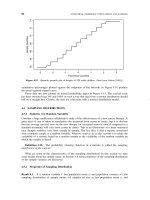
Figure 4.16 Three sampling distributions for means of random samples of size 1, 2, and 4 from a N(0, 1)
population.
Result 4.2 basically states that if Y is normally distributed, then
Y , the mean of a random
sample, is normally distributed. Result 4.1 then specifies the mean and variance of the sampling
distribution. Result 4.2 implies that as the sample size increases, the (normal) distribution of the
sample mean becomes more and more “pinched.” Figure 4.16 shows three sampling distributions
for means of random samples of size 1, 2, and 4.
What is the probability that the average IQ of a class of 25 students exceeds 106? By
Result 4.2,
Y , the average of 25 IQs, is normally distributed with mean µ = 100 and standard
error σ/
√
n = 15/
√
25 = 3. Hence the probability that Y>106 can be calculated as
P [
Y ≥ 106] = P

Z ≥
106 −100
3


= P [Z ≥ 2]
= 1 − 0.9772
= 0.0228
So approximately 2% of average IQs of classes of 25 students will exceed 106. This can be
compared with the probability that a single person’s IQ exceeds 106:
P [Y>106] = P

Z>
6
15

= P [Z>0.4] = 0.3446
The final result we want to state is known as the central limit theorem.
Result 4.3. If a random variable Y has population mean µ and population variance σ
2
,the
sample mean
Y , based on n observations, is approximately normally distributed with mean µ
and variance σ
2
/n, for sufficiently large n.
This is a remarkable result and the most important reason for the central role of the normal
distribution in statistics. What this states basically is that means of random samples from any
distribution (with mean and variance) will tend to be normally distributed as the sample size
becomes sufficiently large. How large is “large”? Consider the distributions of Figure 4.2. Sam-
ples of six or more from the first three distributions will have means that are virtually normally
INFERENCE ABOUT THE MEAN OF A POPULATION 85
0.0 0.5 1.0 1.5 2.0 2.5 3.0
0.0 0.5 1.0 1.5
Sample Mean

Density
n = 5
n = 20
Figure 4.17 Sampling distributions of means of 5 and 20 observations when the parent distribution is
exponential.
distributed. The fourth distribution will take somewhat larger samples before approximate nor-
mality is obtained; n must be around 25 or 30. Figure 4.17 is a more skewed figure that shows
the sampling distributions of means of samples of various sizes drawn from Figure 4.2(d).
The central limit theorem provides some reassurance when we are not certain whether obser-
vations are normally distributed. The means of reasonably sized samples will have a distribution
that is approximately normal. So inference procedures based on the sample means can often
use the normal distribution. But you must be careful not to impute normality to the original
observations.
4.6 INFERENCE ABOUT THE MEAN OF A POPULATION
4.6.1 Point and Interval Estimates
In this section we discuss inference about the mean of a population when the population variance
is known. The assumption may seem artificial, but sometimes this situation will occur. For
example, it may be that a new treatment alters the level of a response variable but not its
variability, so that the variability can be assumed to be known from previous experiments. (In
Section 4.8 we discuss a method for comparing the variability of an experiment with previous
established variability; in Chapter 5 the problem of inference when both population mean and
variance are unknown is considered.)
To put the problem more formally, we have a random variable Y with unknown population
mean µ. A random sample of size n is taken and inferences about µ are to be made on the basis
of the sample. We assume that the population variance is known; denote it by σ
2
. Normality
will also be assumed; even when the population is not normal, we may be able to appeal to the
central limit theorem.
A “natural” estimate of the population mean µ is the sample mean

Y . It is a natural estimate
of µ because we know that
Y is normally distributed with the same mean, µ, and variance σ
2
/n.
Even if Y is not normal,
Y is approximately normal on the basis of the central limit theorem.
The statistic
Y is called a point estimate since we estimate the parameter µ by a single value
or point.
Now the question arises: How precise is the estimate? How can we distinguish between
two samples of, say, 25 and 100 observations? Both may give the same—or approximately the
same—sample mean, but we know that the mean based on the 100 observations is more accurate,
that is, has a smaller standard error. One possible way of summarizing this information is to give
the sample mean and its standard error. This would be useful for comparing two samples. But
this does not seem to be a useful approach in considering one sample and its information about
86 STATISTICAL INFERENCE: POPULATIONS AND SAMPLES
the parameter. To use the information in the sample, we set up an interval estimate as follows:
Consider the quantity µ  (1.96)σ/
√
n. It describes the spread of sample means; in particular,
95% of means of samples of size n will fall in the interval [µ −1.96σ/
√
n, µ +1.96σ/
√
n]. The
interval has the property that as n increases, the width decreases (refer to Section 4.5 for further
discussion). Suppose that we now replace µ by its point estimate,
Y . How can we interpret the
resulting interval? Since the sample mean,

Y , varies from sample to sample, it cannot mean that
95% of the sample means will fall in the interval for a specific sample mean. The interpretation
is that the probability is 0.95 that the interval straddles the population mean. Such an interval
is referred to as a 95% confidence interval for the population mean, µ. We now formalize this
definition.
Definition 4.17. A 100(1 −α)% confidence interval for the mean µ of a normal population
(with variance known) based on a random sample of size n is
Y  z
1−α/2
σ
√
n
where z
1−α/2
is the value of the standard normal deviate such that 100(1 −α)% of the area falls
within z
1−α/2
.
Strictly speaking, we should write

Y + z
α/2
σ
√
n
,
Y + z
1−α/2
σ
√

n

but by symmetry, z
α/2
=−z
1−α/2
, so that it is quicker to use the expression above.
Example 4.8. In Section 3.3.1 we discussed the age at death of 78 cases of crib death
(SIDS) occurring in King County, Washington, in 1976–1977. Birth certificates were obtained
for these cases and birthweights were tabulated. Let Y = birthweight in grams. Then, for these
78 cases,
Y = 2993.6 = 2994 g. From a listing of all the birthweights, it is known that the
standard deviation of birthweight is about 800 g (i.e., σ = 800 g). A 95% confidence interval
for the mean birthweight of SIDS cases is calculated to be
2994 (1.96)

800
√
78

or 2994 (1.96)(90.6) or 2994 178
producing a lower limit of 2816 g and an upper limit of 3172 g. Thus, on the basis of these
data, we are 95% confident that we have straddled the population mean, µ, of birthweight of
SIDS infants by the interval (2816, 3172).
Suppose that we had wanted to be more confident: say, a level of 99%. The value of Z now
becomes 2.58 (from Table A.2), and the corresponding limits are 2994  (2.58)(800/
√
78),or
(2760, 3228). The width of the 99% confidence interval is greater than that of the 95% confidence
interval (468 g vs. 356 g), the price we paid for being more sure that we have straddled the

population mean.
Several comments should be made about confidence intervals:
1. Since the population mean µ is fixed, it is not correct to say that the probability is 1 −α
that µ is in the confidence interval once it i s computed; that probability is zero or 1. Either
the mean is in the interval and the probability is equal to 1, or the mean is not in the
interval and the probability is zero.
INFERENCE ABOUT THE MEAN OF A POPULATION 87
2. We can increase our confidence that the interval straddles the population mean by decreas-
ing α, hence increasing Z
1−α/2
. We can take values from Table A.2 to construct the
following confidence levels:
Confidence Level Z -Value
90% 1.64
95% 1.96
99% 2.58
99.9% 3.29
The effect of increasing the confidence level will be to increase the width of the confidence
interval.
3. To decrease the width of the confidence interval, we can either decrease the confidence
level or increase the sample size. The width of the interval is 2z
1−α/2
σ/
√
n. For a fixed
confidence level the width is essentially a function of σ/
√
n, the standard error of the
mean. To decrease the width by a factor of, say, 2, the sample size must be increased by
a factor of 4, analogous to the discussion in Section 4.5.2.

4. Confidence levels are usually taken to be 95% or 99%. These levels are a matter of
convention; there are no theoretical reasons for choosing these values. A rough rule to
keep in mind is that a 95% confidence interval is defined by the sample mean 2 standard
errors (not standard deviations).
4.6.2 Hypothesis Testing
In estimation, we start with a sample statistic and make a statement about the population param-
eter: A confidence interval makes a probabilistic statement about straddling the population
parameter. In hypothesis testing, we start by assuming a value for a parameter, and a prob-
ability statement is made about the value of the corresponding statistic. In this section, as in
Section 4.6.1, we assume that the population variance is known and that we want to make infer-
ences about the mean of a normal population on the basis of a sample mean. The basic strategy
in hypothesis testing is to measure how far an observed statistic is from a hypothesized value
of the parameter. If the distance is “great” (Figure 4.18) we would argue that the hypothesized
parameter value is inconsistent with the data and we would be inclined to reject the hypothesis
(we could be wrong, of course; rare events do happen).
To interpret the distance, we must take into account the basic variability (σ
2
) of the obser-
vations and the size of the sample (n) on which the statistic is based. As a rough rule of thumb
that is explained below, if the observed value of the statistic is more than two standard errors
from the hypothesized parameter value, we question the truth of the hypothesis.
To continue Example 4.8, the mean birthweight of the 78 SIDS cases was 2994 g. The
standard deviation σ
0
was assumed to be 800 g, and the standard error σ/
√
n = 800/
√
78 =
90.6 g. One question that comes up in the study of SIDS is whether SIDS cases tend to have

a different birthweight than the general population. For the general population, the average
birthweight is about 3300 g. Is the sample mean value of 2994 g consistent with this value?
Figure 4.19 shows that the distance between the two values is 306 g. The standard error is 90.6,
Figure 4.18 Great distance from a hypothesized value of a parameter.
88 STATISTICAL INFERENCE: POPULATIONS AND SAMPLES
Figure 4.19 Distance between the two values is 306 g.
so the observed value is 306/90.6 = 3.38 standard errors from the hypothesized population
mean. By the rule we stated, the distance is so great that we would conclude that the mean
of the sample of SIDS births is inconsistent with the mean value in the general population.
Hence, we would conclude that the SIDS births come from a population with mean birthweight
somewhat less than that of the general population. (This raises more questions, of course: Are the
gestational ages comparable? What about the racial composition? and so on.) The best estimate
we have of the mean birthweight of the population of SIDS cases is the sample mean: in this
case, 2994 g, about 300 g lower than that for the normal population.
Before introducing some standard hypothesis testing terminology, two additional points
should be made:
1. We have expressed “distance” in terms of number of standard errors from the hypothesized
parameter value. Equivalently, we can associate a tail probability with the observed value
of the statistic. For the sampling situation described above, we know that the sample mean
Y is normally distributed with standard error σ/
√
n. As Figure 4.20 indicates, the farther
away the observed value of the statistic is from the hypothesized parameter value, the
smaller the area (probability) in the tail. This tail probability is usually called the p-value.
For example (using Table A.2), the area to the right of 1.96 standard errors is 0.025; the
area to the right of 2.58 standard errors is 0.005. Conversely, if we specify the area, the
number of standard errors will be determined.
2. Suppose that we planned before doing the statistical test that we would not question
the hypothesized parameter value if the observed value of the statistic fell within, say,
two standard errors of the parameter value. We could divide the sample space for the

statistic (i.e., the real line) into three regions as shown in Figure 4.21. These regions
could have been set up before the value of the statistic was observed. All that needs to be
determined then is in which region the observed value of the statistic falls to determine
if it is consistent with the hypothesized value.
Figure 4.20 The farther away the observed value of a statistic from the hypothesized value of a parameter,
the smaller the area in the tail.
INFERENCE ABOUT THE MEAN OF A POPULATION 89
Figure 4.21 Sample space for the statistic.
We now formalize some of these concepts:
Definition 4.18. A null hypothesis specifies a hypothesized real value, or values, for a
parameter (see Note 4.15 for further discussion).
Definition 4.19. The rejection region consists of the set of values of a statistic for which
the null hypothesis is rejected. The values of the boundaries of the region are called the critical
values.
Definition 4.20. A Type I error occurs when the null hypothesis is rejected when, in fact,
it is true. The significance level is the probability of a Type I error when the null hypothesis
is true.
Definition 4.21. An alternative hypothesis specifies a real value or range of values for a
parameter that will be considered when the null hypothesis is rejected.
Definition 4.22. A Type II error occurs when the null hypothesis is not rejected when it is
false.
Definition 4.23. The power of a test is the probability of rejecting the null hypothesis when
it is false.
Cartoon 4.1 Testing some hypotheses can be tricky. (From American Scientist, March–April 1976.)
90 STATISTICAL INFERENCE: POPULATIONS AND SAMPLES
Definition 4.24. The p-value in a hypothesis testing situation is that value of p,0≤ p ≤ 1,
such that for α>pthe test rejects the null hypothesis at significance level α,andforα<p
the test does not reject the null hypothesis. Intuitively, the p-value is the probability under the
null hypothesis of observing a value as unlikely or more unlikely than the value of the test
statistic. The p-value is a measure of the distance from the observed statistic to the value of the

parameter specified by the null hypothesis.
Notation
1. The null hypothesis is denoted by H
0
the alternative hypothesis by H
A
.
2. The probability of a Type I error is denoted by α, the probability of a Type II error by β.
The power is then
power = 1 −probability of Type II error
= 1 −β
Continuing Example 4.8, we can think of our assessment of the birthweight of SIDS babies
as a type of decision problem illustrated in the following layout:
State of Nature SIDS Birthweights
Decision SIDS Birthweights Same as Normal Not the Same
Same as normal Correct (1 −α) Type II error (β)
Not the same Type I error (α) Correct (1 −β)
This illustrates the two types of errors that can be made depending on our decision and the
state of nature. The null hypothesis for this example can be written as
H
0
: µ = 3300 g
and the alternative hypothesis written as
H
A
: µ = 3300 g
Suppose that we want to reject the null hypothesis when the sample mean
Y is more than
two standard errors from the H
0

value of 3300 g. The standard error is 90.6 g. The rejection
region is then determined by 3300  (2)(90.6) or 3300 181.
We can then set up the hypothesis-testing framework as indicated in Figure 4.22. The rejection
region consists of values to the left of 3119 g (i.e., µ −2σ/
√
n) and to the right of 3481 g (i.e.,
µ + 2σ/
√
n). The observed value of the statistic, Y = 2994 g, falls in the rejection region,
and we therefore reject the null hypothesis that SIDS cases have the same mean birthweight as
normal children. On the basis of the sample value observed, we conclude that SIDS babies tend
to weigh less than normal babies.
Figure 4.22 Hypothesis-testing framework for birthweight assessment.
INFERENCE ABOUT THE MEAN OF A POPULATION 91
The probability of a Type I error is the probability that the mean of a sample of 78 observations
from a population with mean 3300 g is less than 3119 g or greater than 3481 g:
P [3119 ≤
Y ≤ 3481] = P

3119 −3300
90.6
≤ Z ≤
3481 −3300
90.6

= P [−2 ≤ Z ≤+2]
where Z is a standard normal deviate.
From Table A.1,
P [Z ≤ 2] = 0.9772
so that

1 −P [−2 ≤ Z ≤ 2] = (2)(0.0228) = 0.0456
the probability of a Type I error. The probability is 0.0455 from the two-sided p-value of
Table A.1. The difference relates to rounding.
The probability of a Type II error can be computed when a value for the parameter under
the alternative hypothesis is specified. Suppose that for these data the alternative hypothesis is
H
A
: µ = 3000 g
this value being suggested from previous studies. To calculate the probability of a Type II
error—and the power—we assume that
Y , the mean of the 78 observations, comes from a
normal distribution with mean 3000 g and standard error as before, 90.6 g. As Figure 4.23
indicates, the probability of a Type II error is the area over the interval (3119, 3481). This can
be calculated as
P [Type II error] = P [3119 ≤
Y ≤ 3481]
= P

3119 −3000
90.6
≤ Z ≤
3481 −3000
90.6

.
= P [1.31 ≤ Z ≤ 5.31]
.
= 1 − 0.905
.
= 0.095

So β = 0.095 and the power is 1 − β = 0.905. Again, these calculations can be made
before any data are collected, and they say that if the SIDS population mean birthweight were
3000 g and the normal population birthweight 3300 g, the probability is 0.905 that a mean from
a sample of 78 observations will be declared significantly different from 3300 g.
Figure 4.23 Probability of a Type II error.
92 STATISTICAL INFERENCE: POPULATIONS AND SAMPLES
Let us summarize the analysis of this example:
Hypothesis-testing setup
(no data taken)






















H
0
: µ = 3300 g
H
A
: µ = 3000 g
σ = 800 g (known)
n = 78
rejection region: 2 standard errors from 3000 g
α = 0.0456
β = 0.095
1 −β = 0.905
Observe:
Y = 2994
Conclusion: Reject H
0
The value of α is usually specified beforehand: The most common value is 0.05, some-
what less common values are 0.01 or 0.001. Corresponding to the confidence level in interval
estimation, we have the significance level in hypothesis testing. The significance level is often
expressed as a percentage and defined to be 100α%. Thus, for α = 0.05, the hypothesis test is
carried out at the 5%, or 0.05, significance level.
The use of a single symbol β for the probability of a Type II error is standard but a bit
misleading. We expect β to stand for one number in the same way that α stands for one number.
In fact, β is a function whose argument is the assumed true value of the parameter being tested.
For example, in the context of H
A
: µ = 3000 g, β is a function of µ and could be written
β(µ). It follows that the power is also a function of the true parameter: power = 1 − β(µ).
Thus one must specify a value of µ to compute the power.
We finish this introduction to hypothesis testing with a discussion of the one- and two-tailed

test. These are related to the choice of the rejection region. Even if α is specified, there is an
infinity of rejection regions such that the area over the region is equal to α. Usually, only two
types of regions are considered as shown in Figure 4.24. A two-tailed test is associated with a
Figure 4.24 Two types of regions considered in hypothesis testing.
CONFIDENCE INTERVALS VS. TESTS OF HYPOTHESES 93
Figure 4.25 Start of the rejection region in a one-tailed test.
rejection region that extends both to the left and to the right of the hypothesized parameter value.
A one-tailed test is associated with a region to one side of the parameter value. The alternative
hypothesis determines the type of test to be carried out. Consider again the birthweight of SIDS
cases. Suppose we know that if the mean birthweight of these cases is not the same as that of
normal infants (3300 g), it must be less; it is not possible for it to be more. In that case, if the
null hypothesis is false, we would expect the sample mean to be below 3300 g, and we would
reject the null hypothesis for values of
Y below 3300 g. We could then write the null hypothesis
and alternative hypothesis as follows:
H
0
: µ = 3300 g
H
A
: µ<3300 g
We would want to carry out a one-tailed test in this case by setting up a rejection region to
the left of the parameter value. Suppose that we want to test at the 0.05 level, and we only want
to reject for values of
Y below 3300 g. From Table A.2 we see that we must locate the start
of the rejection region 1.64 standard errors to the left of µ = 3300 g, as shown in Figure 4.25.
The value is 3300 −(1.64)(800/
√
78) or 3300 −(1.64)(90.6) = 3151 g.
Suppose that we want a two-tailed test at the 0.05 level. The Z-value (Table A.2) is now

1.96, which distributes 0.025 in the left tail and 0.025 in the right tail. The corresponding values
for the critical region are 3300 (1.96)(90.6) or (3122, 3478), producing a region very similar
to the region calculated earlier.
The question is: When should you do a one-tailed test and when a two-tailed test? As
was stated, the alternative hypothesis determines this. An alternative hypothesis of the form
H
A
: µ = µ
0
is called two-sided and will require a two-tailed test. Similarly, the alternative
H
A
: µ<µ
0
is called one-sided and will lead to a one-tailed test. So should the alternative
hypothesis be one- or two-sided? The experimental situation will determine this. For example,
if nothing is known about the effect of a proposed therapy, the alternative hypothesis should
be made two-sided. However, if it is suspected that a new therapy will do nothing or increase
a response level, and if there is no reason to distinguish between no effect and a decrease in
the response level, the test should be one-tailed. The general rule is: The more specific you can
make the experiment, the greater the power of the test (see Fleiss et al. [2003, Sec. 2.4]). (See
Problem 4.33 to convince yourself that the power of a one-tailed test is greater if the alternative
hypothesis specifies the situation correctly.)
4.7 CONFIDENCE INTERVALS VS. TESTS OF HYPOTHESES
You may have noticed that there is a very close connection between the confidence intervals and
the tests of hypotheses that we have constructed. In both approaches we have used the standard
normal distribution and the quantity α.
In confidence intervals we:
1. Specify the confidence level (1 −α).
94 STATISTICAL INFERENCE: POPULATIONS AND SAMPLES

2. Read z
1−α/2
from a standard normal table.
3. Calculate
Y  z
1−α/2
σ/
√
n.
In hypothesis testing we:
1. Specify the null hypothesis (H
0
: µ = µ
0
).
2. Specify α, the probability of a Type I error.
3. Read z
1−α/2
from a standard normal table.
4. Calculate µ
0
 z
1−α/2
σ/
√
n.
5. Observe
Y ; reject or accept H
0
.

The two approaches can be represented pictorially as shown in Figure 4.26. It is easy to
verify that if the confidence interval does not straddle µ
0
(as is the case in the figure),
Y will
fall in the rejection region, and vice versa. Will this always be the case? The answer is “yes.”
When we are dealing with inference about the value of a parameter, the two approaches will
give the same answer. To show the equivalence algebraically, we start with the key inequality
P

−z
1−α/2
≤
Y − µ
σ/
√
n
≤ z
1−α/2

= 1 −α
If we solve the inequality for
Y ,weget
P

µ −
z
1−α/2
σ
√

n
≤
Y ≤ µ +
z
1−α/2
√
n

= 1 −α
Given a value µ = µ
0
, the statement produces a region (µ
0
 z
1−α/2
σ/
√
n) within which
100(1 −α)% of sample means fall. If we solve the inequality for µ,weget
P

Y −
z
1−α/2
σ
√
n
≤ µ ≤
Y +
z

1−α/2
σ
√
n

= 1 −α
This is a confidence interval for the population mean µ. In Chapter 5 we examine this approach
in more detail and present a general methodology.
Figure 4.26 Confidence intervals vs. tests of hypothesis.
INFERENCE ABOUT THE VARIANCE OF A POPULATION 95
If confidence intervals and hypothesis testing are but two sides of the same coin, why
bother with both? The answer is (to continue the analogy) that the two sides of the coin are
not the same; there is different information. The confidence interval approach emphasizes the
precision of the estimate by means of the width of the interval and provides a point estimate
for the parameter, regardless of any hypothesis. The hypothesis-testing approach deals with the
consistency of observed (new) data with the hypothesized parameter value. It gives a probability
of observing the value of the statistic or a more extreme value. In addition, it will provide a
method for estimating sample sizes. Finally, by means of power calculations, we can decide
beforehand whether a proposed study is feasible; that is, what is the probability that the study
will demonstrate a difference if a (specified) difference exists?
You should become familiar with both approaches to statistical inference. Do not use one to
the exclusion of another. In some research fields, hypothesis testing has been elevated to the only
“proper” way of doing inference; all scientific questions have to be put into a hypothesis-testing
framework. This is absurd and stultifying, particularly in pilot studies or investigations into
uncharted fields. On the other hand, not to consider possible outcomes of an experiment and the
chance of picking up differences is also unbalanced. Many times it will be useful to specify very
carefully what is known about the parameter(s) of interest and to specify, in perhaps a crude
way, alternative values or ranges of values for these parameters. If it is a matter of emphasis,
you should stress hypothesis testing before carrying out a study and estimation after the study
has been done.

4.8 INFERENCE ABOUT THE VARIANCE OF A POPULATION
4.8.1 Distribution of the Sample Variance
In previous sections we assumed that the population variance of a normal distribution was
known. In this section we want to make inferences about the population variance on the basis
of a sample variance. In making inferences about the population mean, we needed to know
the sampling distribution of the sample mean. Similarly, we need to know the sampling dis-
tribution of the sample variance in order to make inferences about the population variance;
analogous to the statement that for a normal random variable, Y , with sample mean
Y ,the
quantity
Y − µ
σ/
√
n
has a normal distribution with mean 0 and variance 1. We now state a result about the quantity
(n − 1)s
2
/σ
2
. The basic information is contained in the following statement:
Result 4.4. If a random variable Y is normally distributed with mean µ and variance σ
2
,
then for a random sample of size n the quantity (n −1)s
2
/σ
2
has a chi-square distribution with
n −1 degrees of freedom.
Each distribution is indexed by n −1 degrees of freedom. Recall that the sample variance is

calculated by dividing

(y −
y)
2
by n − 1, the degrees of freedom.
The chi-square distribution is skewed; the amount of skewness decreases as the degrees of
freedom increases. Since (n−1)s
2
/σ
2
can never be negative, the sample space for the chi-square
distribution is the nonnegative part of the real line. Several chi-square distributions are shown
in Figure 4.27. The mean of a chi-square distribution is equal to the degrees of freedom, and
96 STATISTICAL INFERENCE: POPULATIONS AND SAMPLES
Figure 4.27 Chi-square distributions.
the variance is twice the degrees of the freedom. Formally,
E

(n − 1)s
2
σ
2

= n − 1(1)
var

(n − 1)s
2
σ

2

= 2(n − 1) (2)
It may seem somewhat strange to talk about the variance of the sample variance, but under
repeated sampling the sample variance will vary from sample to sample, and the chi-square
distribution describes this variation if the observations are from a normal distribution.
Unlike the normal distribution, a tabulation of the chi-square distribution requires a separate
listing for each degree of freedom. In Table A.3, a tabulation is presented of percentiles of the
chi-square distribution. For example, 95% of chi-square random variables with 10 degrees of
freedom have values less than or equal to 18.31. Note that the median (50th percentile) is very
close to the degrees of freedom when the number of the degrees of freedom is 10 or more.
The symbol for a chi-square random variable is χ
2
, the Greek lowercase letter chi, to the
power of 2. So we usually write χ
2
= (n − 1)s
2
/σ
2
. The degrees of freedom are usually
indicated by the Greek lowercase letter ν (nu). Hence, χ
2
ν
is a symbol for a chi-square random
variable with ν degrees of freedom. It is not possible to maintain the notation of using a capital
letter for a variable and the corresponding lowercase letter for the value of the variable.
4.8.2 Inference about a Population Variance
We begin with hypothesis testing. We have a sample of size n from a normal distribution, the
sample variance s

2
has been calculated, and we want to know whether the value of s
2
observed
is consistent with a hypothesized population value σ
2
0
, perhaps known from previous research.
Consider the quantity
χ
2
=
(n − 1)s
2
σ
2
INFERENCE ABOUT THE VARIANCE OF A POPULATION 97
If s
2
is very close to σ
2
, the ratio s
2
/σ
2
is close to 1; if s
2
differs very much from σ
2
, the ratio

is either very large or very close to 0: This implies that χ
2
= (n −1)s
2
/σ
2
is either very large
or very small, and we would want to reject the null hypothesis. This procedure is analogous to a
hypothesis test about a population mean; we measured the distance of the observed sample mean
from the hypothesized value in units of standard errors; in this case we measure the “distance”
in units of the hypothesized variance.
Example 4.9. The SIDS cases discussed in Section 3.3.1 were assumed to come from a
normal population with variance σ
2
= (800)
2
. To check this assumption, the variance, s
2
,is
calculated for the first 11 cases occurring in 1969. The birthweights (in grams) were
3374, 3515, 3572, 2977, 4111, 1899, 3544, 3912, 3515, 3232, 3289
The sample variance is calculated to be
s
2
= (574.3126 g)
2
The observed value of the chi-square quantity is
χ
2
=

(11 −1)(574.3126)
2
(800)
2
= 5.15 with 10 degrees of freedom
Figure 4.14 illustrates the chi-square distribution with 10 degrees of freedom. The 2.5th and
97.5th percentiles are 3.25 and 20.48 (see Table A.3). Hence, 95% of chi-square values will fall
between 3.25 and 20.48.
If we follow the usual procedure of setting our significance level at α = 0.05, we will not
reject the null hypothesis that σ
2
= (800 g)
2
, since the observed value χ
2
= 5.15 is less extreme
than 3.25. Hence, there is not sufficient evidence for using a value of σ
2
not equal to 800 g.
As an alternative to setting up the rejection regions formally, we could have noted, using
Table A.3, that the observed value of χ
2
= 5.15 is between the 5th and 50th percentiles, and
therefore the corresponding two-sided p-value is greater than 0.10.
A 100(1 − α)% confidence interval is constructed using the approach of Section 4.7. The
key inequality is
P [χ
2
α/2
≤ χ

2
≤ χ
2
1−α/2
] = 1 −α
The degrees of freedom are not indicated but assumed to be n −1. The values χ
2
α/2
and χ
2
1−α/2
are chi-square values such that 1 −α of the area is between them. (In Figure 4.14, these values
are 3.25 and 20.48 for 1 −α = 0.95.)
The quantity χ
2
is now replaced by its equivalent, (n − 1)s
2
/σ
2
,sothat
P

χ
2
α/2
≤
(n − 1)s
2
σ
2

≤ χ
2
1−α/2

= 1 −α
If we solve for σ
2
, we obtain a 100(1 −α)% confidence interval for the population variance. A
little algebra shows that this is
P

(n − 1)s
2
χ
2
1−α/2
≤ σ
2
≤
(n − 1)s
2
χ
2
α/2

= 1 −α
98 STATISTICAL INFERENCE: POPULATIONS AND SAMPLES
0 5 10 15 20 25 30
0.00 0.02 0.04 0.06 0.08 0.10
Density

P(c
2
10
< 3.25) = 0.025
P(c
2
10
> 20.48) = 0.025
Figure 4.28 Chi-square distribution with 10 degrees of freedom.
Given an observed value of s
2
, the confidence interval required can now be calculated.
To continue our example, the variance for the 11 SIDS cases above is s
2
= (574.3126 g)
2
.
For 1 − α = 0.95, the values of χ
2
are (see Figure 4.28)
χ
2
0.025
= 3.25,χ
2
0.975
= 20.48
We can write the key inequality then as
P [3.25 ≤ χ
2

≤ 20.48] = 0.95
The 95% confidence interval for σ
2
can then be calculated:
(10)(574.3126)
2
20.48
≤ σ
2
≤
(10)(574.3126)
2
3.25
and simplifying yields
161,052 ≤ σ
2
≤ 1,014,877
The corresponding values for the population standard deviation are
lower 95% limit for σ =

161, 052 = 401 g
upper 95% limit for σ =

1,014,877 = 1007 g
These are rather wide limits. Note that they include the null hypothesis value of σ = 800 g.
Thus, the confidence interval approach leads to the same conclusion as the hypothesis-testing
approach.
NOTES
4.1 Definition of Probability
The relative frequency definition of probability was advanced by von Mises, Fisher, and others

(see Hacking [1965]). A radically different view is held by the personal or subjective school,
NOTES 99
exemplified in the work of De Finetti, Savage, and Savage. According to this school, probability
reflects subjective belief and knowledge that can be quantified in terms of betting behavior.
Savage [1968] states: “My probability for the event A under circumstances H is the amount of
money I am indifferent to betting on A in an elementary gambling situation.” What does Savage
mean? Consider the thumbtack experiment discussed in Section 4.3.1. Let the event A be that
the thumbtack in a single toss falls ⊥. The other possible outcome is ⊤; call this event B.You
are to bet a dollars on A and b dollars on B, such that you are indifferent to betting either on
A or on B (you must bet). You clearly would not want to put all your money on A; then you
would prefer outcome A. There is a split, then, in the total amount, a +b, to be bet so that you
are indifferent to either outcome A or B.Thenyour probability of A, P [A], is
P [A] =
b
a + b
If the total amount to be bet is 1 unit, you would split it 1 −P , P ,where0≤ P ≤ 1, so that
P [A] =
P
1 −P + P
= P
The bet is a device to link quantitative preferences for amounts b and a of money, which are
assumed to be well understood, to preferences for degrees of certainty, which we are trying to
quantify. Note that Savage is very careful to require the estimate of the probability to be made
under as specified circumstances. (If the thumbtack could land, say, ⊤ on a soft surface, you
would clearly want to modify your probability.) Note also that betting behavior is a definition
of personal probability rather than a guide for action. In practice, one would typically work
out personal probabilities by comparison to events for which the probabilities were already
established (Do I think this event is more or less likely than a coin falling heads?) rather than
by considering sequences of bets.
This definition of probability is also called personal probability. An advantage of this view

is that it can discuss more situations than the relative frequency definition, for example: the
probability (rather, my probability) of life on Mars, or my probability that a cure for cancer will
be found. You should not identify personal probability with the irrational or whimsical. Personal
probabilities do utilize empirical evidence, such as the behavior of a tossed coin. In particular,
if you have good reason to believe that the relative frequency of an event is P , your personal
probability will also be P . It is possible to show that any self-consistent system for choosing
between uncertain outcomes corresponds to a set of personal probabilities.
Although different individuals will have different personal probabilities for an event, the way
in which those probabilities are updated by evidence is the same. It is possible to develop statis-
tical analyses that summarize data in terms of how it should change one’s personal probabilities.
In simple analyses these Bayesian methods are more difficult to use than those based on relative
frequencies, but the situation is reversed for some complex models. The use of Bayesian statis-
tics is growing in scientific and clinical research, but it is still not supported by most standard
software. An introductory discussion of Bayesian statistics is given by Berry [1996], and more
advanced books on practical data analysis include Gelman et al. [1995] and Carlin and Louis
[2000]. There are other views of probability. For a survey, see the books by Hacking [1965]
and Barnett [1999] and references therein.
4.2 Probability Inequalities
For the normal distribution, approximately 68% of observations are within one standard deviation
of the mean, and 95% of observations are within two standard deviations of the mean. If the
distribution is not normal, a weaker statement can be made: The proportion of observations
100 STATISTICAL INFERENCE: POPULATIONS AND SAMPLES
within K standard deviations of the mean is greater than or equal to (1 − 1/K
2
); notationally,
for a variable Y ,
P

−K ≤
Y − E(Y)

σ
≤ K

≤ 1 −
1
K
2
where K is the number of standard deviations from the mean. This is a version of Chebyshev’s
inequality. For example, this inequality states that at least 75% of the observations fall within
two standard deviations of the mean (compared to 95% for the normal distribution). This is not
nearly as stringent as the first result stated, but it is more general. If the variable Y can take on
only positive values and the mean of Y is µ, the following inequality holds:
P [Y ≤ y] ≤ 1 −
µ
y
This inequality is known as the Markov inequality.
4.3 Inference vs. Decision
The hypothesis tests discussed in Sections 4.6 and 4.7 can be thought of as decisions that are
made with respect to a value of a parameter (or state of nature). There is a controversy in
statistics as to whether the process of inference is equivalent to a decision process. It seems that
a “decision” is sometimes not possible in a field of science. For example, it is not possible at
this point to decide whether better control of insulin levels will reduce the risk of neuropathy
in diabetes mellitus. In this case and others, the types of inferences we can make are more
tenuous and cannot really be called decisions. For an interesting discussion, see Moore [2001].
This is an excellent book covering a variety of statistical topics ranging from ethical issues in
experimentation to formal statistical reasoning.
4.4 Representative Samples
A random sample from a population was defined in terms of repeated independent trials or
drawings of observations. We want to make a distinction between a random and a representative
sample. A random sample has been defined in terms of repeated independent sampling from a

population. However (see Section 4.3.2), cancer patients treated in New York are clearly not a
random sample of all cancer patients in the world or even in the United States. They will differ
from cancer patients in, for instance, Great Britain in many ways. Yet we do frequently make
the assumption that if a cancer treatment worked in New York, patients in Great Britain can also
benefit. The experiment in New York has wider applicability. We consider that with respect to
the outcome of interest in the New York cancer study (e.g., increased survival time), the New
York patients, although not a random sample, constitute a representative sample. That is, the
survival times are a random sample from the population of survival times.
It is easier to disprove randomness than representativeness. A measure of scientific judgment
is involved in determining the latter. For an interesting discussion of the use of the word
representative, see the papers by Kruskal and Mosteller [1979a–c].
4.5 Multivariate Populations
Usually, we study more than one variable. The Winkelstein et al. [1975] study (see Example 4.1)
measured diastolic and systolic blood pressures, height, weight, and cholesterol levels. In the
study suggested in Example 4.2, in addition to IQ, we would measure physiological and psycho-
logical variables to obtain a more complete picture of the effect of the diet. For completeness
we therefore define a multivariate population as the set of all possible values of a specified set
of variables (measured on the objects of interest). A second category of topics then comes up:
NOTES 101
relationships among the variables. Words such as association and correlation come up in this
context. A discussion of these topics begins in Chapter 9.
4.6 Sampling without Replacement
We want to select two patients at random from a group of four patients. The same patient cannot
be chosen twice. How can this be done? One procedure is to write each name on a slip of paper,
put the four slips of paper in a hat, stir the slips of paper, and—without looking—draw out
two slips. The patients whose names are on the two slips are then selected. This is known as
sampling without replacement. (For the procedure to be fair, we require that the slips of paper
be indistinguishable and well mixed.) The events “outcome on first draw” and “outcome on
second draw” are clearly not independent. If patient A is selected in the first draw, she is no
longer available for the second draw. Let the patients be labeled A, B, C,andD. Let the symbol

AB mean “patient A is selected in the first draw and patient B in the second draw.” Write down
all the possible outcomes; there are 12 of them as follows:
AB BA CA DA
AC BC CB DB
AD BD CD DC
We define the selection of two patients to be random if each of the 12 outcomes is equally
likely, that is, the probability that a particular pair is chosen is 1/12. This definition has intuitive
appeal: We could have prepared 12 slips of paper each with one of the 12 pairs recorded and
drawnout one slip of paper. If the slip of paper is drawn randomly, the probability is 1/12 that
a particular slip will be selected.
One further comment. Suppose that we only want to know which two patients have been
selected (i.e., we are not interested in the order). For example, what is the probability that
patients C and D are selected? This can happen in two ways: CD or DC. These events are
mutually exclusive, so that the required probability is P [CD or DC ] = P [CD] + P [DC] =
1/12 +1/12 = 1/6.
4.7 Pitfalls in Sampling
It is very important to define the population of interest carefully. Two illustrations of rather
subtle pitfalls are Berkson’s fallacy and length-biased sampling. Berkson’s fallacy is discussed
in Murphy [1979] as follows: In many studies, hospital records are reviewed or sampled to
determine relationships between diseases and/or exposures. Suppose that a review of hospital
records is made with respect to two diseases, A and B, which are so severe that they always
lead to hospitalization. Let their frequencies in the population at large be p
1
and p
2
. Then,
assuming independence, the probability of the joint occurrence of the two diseases is p
1
p
2

.
Suppose now that a healthy proportion p
3
of subjects (H ) never go to the hospital; that is,
P [H ] = p
3
. Now write
H as that part of the population that will enter a hospital at some
time; then P [
H ] = 1 −p
3
. By the rule of conditional probability, P [AH ] = P [AH ]/P [H ] =
p
1
/(1 −p
3
). Similarly, P [B
H ] = p
2
/(1 −p
3
) and P [ABH ] = p
1
p
2
/(1 −p
3
), and this is not
equal to P [A
H ]P [BH ] = [p

1
/(1−p
3
)][p
2
/(1−p
3
)], which must be true in order for the two
diseases to be unrelated in the hospital population. Now, you can show that P [AB
H ] <P[AB],
and, quoting Murphy:
The hospital observer will find that they occur together less commonly than would be expected if
they were independent. This is known as Berkson’s fallacy. It has been a source of embarrassment
to many an elegant theory. Thus, cirrhosis of the liver and common cancer are both reasons for
admission to the hospital. Apriori, we would expect them to be less commonly associated in the
hospital than in the population at large. In fact, they have been found to be negatively correlated.
102 STATISTICAL INFERENCE: POPULATIONS AND SAMPLES
Table 4.4 Expected Composition of Visit-Based Sample
in a Hypothetical Population
Type of Patient
Variable Hypertensive Other Total
Number of patients 200 800 1000
Visits per patient per year 12 1 13
Visits contributed 2400 800 3200
Expected number of patients
in a 3% sample of visits
72 24 96
Expected percent of sample 75 25 100
Source: Shepard and Neutra [1977].
(Murphy’s book contains an elegant, readable exposition of probability in medicine; it will

be worth your while to read it.)
A second pitfall deals with the area of length-biased sampling. This means that for a particular
sampling scheme, some objects in the population may be more likely to be selected than others. A
paper by Shepard and Neutra [1977] illustrates this phenomenon in sampling medical visits. Our
discussion is based on that paper. The problem arises when we want to make a statement about a
population of patients that can only be identified by a sample of patient visits. Therefore, frequent
visitors will be more likely to be selected. Consider the data in Table 4.4, which illustrates that
although hypertensive patients make up 20% of the total patient population, a sample based on
visits would consist of 75% hypertensive patients and 25% other.
There are other areas, particularly screening procedures in chronic diseases, that are at risk
for this type of problem. See Shepard and Neutra [1977] for suggested solutions as well as
references to other papers.
4.8 Other Sampling Schemes
In this chapter (and almost all the remainder of the book) we are assuming simple random
sampling, that is, sampling where every unit in the population is equally likely to end up in the
sample, and sampling of different units is independent. A sufficiently large simple random sample
will always be representative of the population. This intuitively plausible result is made precise
in the mathematical result that the empirical cumulative distribution of the sample approaches
the true cumulative distribution of the population as the sample size increases.
There are some important cases where other random sampling strategies are used, trading
increased mathematical complexity for lower costs in obtaining the sample. The main techniques
are as follows:
1. Stratified sampling. Suppose that we sampled 100 births to study low birthweight. We
would expect to see about one set of twins on average, but might be unlucky and not
sample any. As twins are much more likely to have low birthweight, we would prefer a
sampling scheme that fixed the number of twins we observed.
2. Unequal probability sampling. In conjunction with stratified sampling, we might want
to increase the number of twin births that we examined to more than the 1/90 in the
population. We might decide to sample 10 twin births rather than just one.
3. Cluster sampling. In a large national survey requiring face-to-face interviews or clinical

tests, it is not feasible to use a simple random sample, as this would mean that nearly
every person sampled would live in a different town or city. Instead, a number of cities
or counties might be sampled and simple random sampling used within the selected
geographic regions.
NOTES 103
4. Two-phase sampling. It is sometimes useful to take a large initial sample and then take
a smaller subsample to measure more expensive or difficult variables. The probability of
being included in the subsample can then depend on the values of variables measured
at the first stage. For example, consider a study of genetic influences on lung cancer.
Lung cancer is rare, so it would be sensible to use a stratified (case–control) sampling
scheme where an equal number of people with and without lung cancer was sampled. In
addition, lung cancer is extremely rare in nonsmokers. If a first-stage sample asked about
smoking status it would be possible to ensure that the more expensive genetic information
was obtained for a sufficient number of nonsmoker cancer cases as well as smokers with
cancer.
These sampling schemes have two important features in common. The sampling scheme is
fully known in advance, and the sampling is random (even if not with equal probabilities).
These features mean that a valid statistical analysis of the results is possible. Although the
sample is not representative of the population, it is unrepresentative in ways that are fully under
the control of the analyst. Complex probability samples such as these require different analyses
from simple random samples, and not all statistical software will analyze them correctly. The
section on Survey Methods of the American Statistical Association maintains a list of statistical
software that analyzes complex probability samples. It is linked from the Web appendix to this
chapter. There are many books discussing both the statistical analysis of complex surveys and
practical considerations involved in sampling, including Levy and Lemeshow [1999], Lehtonen
and Pahkinen [1995], and Lohr [1999]. Similar, but more complex issues arise in environmental
and ecological sampling, where measurement locations are sampled from a region.
4.9 How to Draw a Random Sample
In Note 4.6 we discussed drawing a random sample without replacement. How can we draw
samples with replacement? Simply, of course, the slips could be put back in the hat. However,

in some situations we cannot collect the total population to be sampled from, due to its size,
for example. One way to sample populations is to use a table of random numbers. Often, these
numbers are really pseudorandom: They have been generated by a computer. Use of such a table
can be illustrated by the following problem: A random sample of 100 patient charts is to be drawn
from a hospital record room containing 45,850 charts. Assume that the charts are numbered in
some fashion from 1 to 45,850. (It is not necessary that they be numbered consecutively or that
the numbers start with 1 and end with 45,850. All that is required is that there is some unique
way of numbering each chart.) We enter the random number table randomly by selecting a page
and a column on the page at random. Suppose that the first five-digit numbers are
06812, 16134, 15195, 84169, and 41316
The first three charts chosen would be chart 06812, 16134, and 15195, in that order. Now what
do we do with the 84169? We can skip it and simply go to 41316, realizing that if we follow
this procedure, we will have to throw out approximately half of the numbers selected.
A second example: A group of 40 animals is to be assigned at random to one of four
treatments A, B, C,andD, with an equal number in each of the treatments. Again, enter the
random number table randomly. The first 10-digit numbers between 1 and 40 will be the numbers
of the animals assigned to treatment A, the second set of 10-digit numbers to treatment B,the
third set to treatment C, and the remaining animals are assigned to treatment D. If a random
number reappears in a subsequent treatment, it can simply be omitted. (Why is this reasonable?)
4.10 Algebra of Expectations
In Section 4.3.3 we discuss random variables, distributions, and expectations of random vari-
ables. We defined E(Y) =

py for a discrete random variable. A similar definition, involving
104 STATISTICAL INFERENCE: POPULATIONS AND SAMPLES
integrals rather than sums, can be made for continuous random variables. We will now state
some rules for working with expectations.
1. If a is a constant, E(aY) = aE(Y).
2. If a and b are constants, E(aY + b) = aE(Y) + b.
3. If X and Y are two random variables, E(X +Y) = E(X) + E(Y).

4. If a and b are constants, E(aX +bY ) = E(aX) + E(bY ) = aE(X) + bE(Y ).
You can demonstrate the first three rules by using some simple numbers and calculating their
average. For example, let y
1
= 2,y
2
= 4, and y
3
= 12. The average is
E(Y) =
1
3
 2 +
1
3
 4 +
1
3
 12 = 6
Two additional comments:
1. The second formula makes sense. Suppose that we measure temperature in
◦
C. The average
is calculated for a series of readings. The average can be transformed to
◦
F by the formula
average in
◦
F =
9

5
 average in
◦
C +32
An alternative approach consists of transforming each original reading to
◦
Fandthen
taking the average. It is intuitive that the two approaches should provide the same answer.
2. It is not true that E(Y
2
) = [E(Y )]
2
. Again, a small example will verify this. Use the
same three values (y
1
= 2,y
2
= 4, and y
3
= 12). By definition,
E(Y
2
) =
2
2
+ 4
2
+ 12
2
3

=
4 +16 + 144
3
=
164
3
= 54.
6
but
[E(Y)]
2
= 6
2
= 36
Can you think of a special case where the equation E(Y
2
) = [E(Y )]
2
is true?
4.11 Bias, Precision, and Accuracy
Using the algebra of expectations, we define a statistic T to be a biased estimate of a parameter
τ if E(T ) = τ. Two typical types of bias are E(T ) = τ + a,wherea is a constant, called
location bias;andE(T ) = bτ,whereb is a positive constant, called scale bias.Asimple
example involves the sample variance, s
2
. A more “natural” estimate of σ
2
might be
s
2

∗
=

(y −
y)
2
n
This statistic differs from the usual sample variance in division by n rather than n − 1. It can
be shown (you can try it) that
E(s
2
∗
) =
n −1
n
σ
2
NOTES 105
Figure 4.29 Accuracy involves the concept of bias.
Hence, s
2
∗
is a biased estimate of σ
2
. The statistic s
2
∗
can be made unbiased by multiplying s
2
∗

by n/(n − 1) (see rule 1 in Note 4.10); that is,
E

n
n −1
s
2
∗

=
n
n −1
n −1
n
σ
2
= σ
2
But n/(n − 1)s
2
∗
= s
2
,sos
2
rather than s
2
∗
is an unbiased estimate of σ
2

. We can now discuss
precision and accuracy. Precision refers to the degree of closeness to each other of a set of
values of a variable; accuracy refers to the degree of closeness of these values to the quantity
(parameter) being measured. Thus, precision is an internal characteristic of a set of data, while
accuracy relates the set to an external standard. For example, a thermometer that consistently
reads a temperature 5 degrees too high may be very precise but will not be very accurate. A
second example of the distribution of hits on a target illustrates these two concepts. Figure 4.29
shows that accuracy involves the concept of bias. Together with Note 4.10, we can now make
these concepts more precise. For simplicity we will refer only to location bias.
Suppose that a statistic T estimates a quantity τ in a biased way; E[T ] = τ + a.The
variance in this case is defined to be E[T −E(T )]
2
. What is the quantity E[T −τ ]
2
? This can
be written as
E[T − τ]
2
= E[T −(τ + a) + a]
2
= E[T −E[T ] +a]
2
E[T − τ]
2
(mean square error)
=
E[T − E[T ]]
2
(variance) +
a

2
(bias)
The quantity E[T −τ ]
2
is called the mean square error. If the statistic is unbiased (i.e., a = 0),
the mean square error is equal to the variance (σ
2
).
4.12 Use of the Word Parameter
We have defined parameter as a numerical characteristic of a population of values of a variable.
One of the basic tasks of statistics is to estimate values of the unknown parameter on the basis of
a sample of values of a variable. There are two other uses of this word. Many clinical scientists
use parameter for variable, as in: “We measured the following three parameters: blood pressure,
106 STATISTICAL INFERENCE: POPULATIONS AND SAMPLES
amount of plaque, and degree of patient satisfaction.” You should be aware of this pernicious
use and strive valiantly to eradicate it from scientific writing. However, we are not sanguine
about its ultimate success. A second incorrect use confuses parameter and perimeter,asin:
“The parameters of the study did not allow us to include patients under 12 years of age.” A
better choice would have been to use the word limitations.
4.13 Significant Digits (continued)
This note continues the discussion of significant digits in Note 3.4. We discussed approximations
to a quantity due to arithmetical operations, measurement rounding, and finally, sampling vari-
ability. Consider the data on SIDS cases of Example 4.11. The mean birthweight of the 78 cases
was 2994 g. The probability was 95% that the interval 2994 178 straddles the unknown quan-
tity of interest: the mean birthweight of the population of SIDS cases. This interval turned out
to be 2816–3172 g, although the last digits in the two numbers are not very useful. In this case
we have carried enough places so that the rule mentioned in Note 3.4 is not applicable. The
biggest source of approximation turns out to be due to sampling. The approximations introduced
by the arithmetical operation is minimal; you can verify that if we had carried more places in
the intermediate calculations, the final confidence interval would have been 2816–3171 g.

4.14 A Matter of Notation
What do we mean by 18 2.6? In many journals you will find this notation. What does it mean?
Is it mean plus or minus the standard deviation, or mean plus or minus the standard error? You
may have to read a paper carefully to find out. Both meanings are used and thus need to be
specified clearly.
4.15 Formula for the Normal Distribution
The formula for the normal probability density function for a normal random variable Y with
mean µ and variance σ
2
is
f(y)=
1
√
2πσ
exp

−
1
2

y − µ
σ

2

Here, π = 3.14159 ,ande is the base of the natural logarithm, e = 2.71828 A standard
normal distribution has µ = 0andσ = 1. The formula for the standard normal random variable,
Z,is
f(z)=
1

√
2π
exp

−
1
2
z
2

Although most statistical packages will do this for you, the heights of the curve can easily be
calculated using a hand calculator. By symmetry, only one half of the range of values has to
be computed [i.e., f(z) = f(−z)]. For completeness in Table 4.5 we give enough points to
enable you to graph f(z). Given any normal variable y with mean µ and variance σ
2
, you can
calculate f(y) by using the relationships
Z =
Y − µ
σ
and plotting the corresponding heights:
f(y)=
1
σ
f(z)
where Z is defined by the relationship above. For example, suppose that we want to graph the
curve for IQ, where we assume that IQ is normal with mean µ = 100 and standard deviation