ROBOTICS Handbook of Computer Vision Algorithms in Image Algebra Part 1 ppsx
Bạn đang xem bản rút gọn của tài liệu. Xem và tải ngay bản đầy đủ của tài liệu tại đây (955.73 KB, 17 trang )
Search Tips
Advanced Search
Handbook of Computer Vision Algorithms in Image Algebra
by Gerhard X. Ritter; Joseph N. Wilson
CRC Press, CRC Press LLC
ISBN: 0849326362 Pub Date: 05/01/96
Search this book:
Preface
Acknowledgments
Chapter 1—Image Algebra
1.1. Introduction
1.2. Point Sets
1.3. Value Sets
1.4. Images
1.5. Templates
1.6. Recursive Templates
1.7. Neighborhoods
1.8. The p-Product
1.9. References
Chapter 2—Image Enhancement Techniques
2.1. Introduction
2.2. Averaging of Multiple Images
2.3. Local Averaging
2.4. Variable Local Averaging
2.5. Iterative Conditional Local Averaging
2.6. Max-Min Sharpening Transform
2.7. Smoothing Binary Images by Association
2.8. Median Filter
2.9. Unsharp Masking
Title
invariant
2.10. Local Area Contrast Enhancement
2.11. Histogram Equalization
2.12. Histogram Modification
2.13. Lowpass Filtering
2.14. Highpass Filtering
2.15. References
Chapter 3—Edge Detection and Boundary Finding Techniques
3.1. Introduction
3.2. Binary Image Boundaries
3.3. Edge Enhancement by Discrete Differencing
3.4. Roberts Edge Detector
3.5. Prewitt Edge Detector
3.6. Sobel Edge Detector
3.7. Wallis Logarithmic Edge Detection
3.8. Frei-Chen Edge and Line Detection
3.9. Kirsch Edge Detector
3.10. Directional Edge Detection
3.11. Product of the Difference of Averages
3.12. Crack Edge Detection
3.13. Local Edge Detection in Three-Dimensional Images
3.14. Hierarchical Edge Detection
3.15. Edge Detection Using K-Forms
3.16. Hueckel Edge Operator
3.17. Divide-and-Conquer Boundary Detection
3.18. Edge Following as Dynamic Programming
3.19. References
Chapter 4—Thresholding Techniques
4.1. Introduction
4.2. Global Thresholding
4.3. Semithresholding
4.4. Multilevel Thresholding
4.5. Variable Thresholding
4.6. Threshold Selection Using Mean and Standard Deviation
4.7. Threshold Selection by Maximizing Between-Class Variance
4.8. Threshold Selection Using a Simple Image Statistic
4.9. References
Chapter 5—Thining and Skeletonizing
5.1. Introduction
5.2. Pavlidis Thinning Algorithm
5.3. Medial Axis Transform (MAT)
5.4. Distance Transforms
5.5. Zhang-Suen Skeletonizing
5.6. Zhang-Suen Transform — Modified to Preserve Homotopy
5.7. Thinning Edge Magnitude Images
5.8. References
Chapter 6—Connected Component Algorithms
6.1. Introduction
6.2. Component Labeling for Binary Images
6.3. Labeling Components with Sequential Labels
6.4. Counting Connected Components by Shrinking
6.5. Pruning of Connected Components
6.6. Hole Filling
6.7. References
Chapter 7—Morphological Transforms and Techniques
7.1. Introduction
7.2. Basic Morphological Operations: Boolean Dilations and Erosions
7.3. Opening and Closing
7.4. Salt and Pepper Noise Removal
7.5. The Hit-and-Miss Transform
7.6. Gray Value Dilations, Erosions, Openings, and Closings
7.7. The Rolling Ball Algorithm
7.8. References
Chapter 8—Linear Image Transforms
8.1. Introduction
8.2. Fourier Transform
8.3. Centering the Fourier Transform
8.4. Fast Fourier Transform
8.5. Discrete Cosine Transform
8.6. Walsh Transform
8.7. The Haar Wavelet Transform
8.8. Daubechies Wavelet Transforms
8.9. References
Chapter 9—Pattern Matching and Shape Detection
9.1. Introduction
9.2. Pattern Matching Using Correlation
9.3. Pattern Matching in the Frequency Domain
9.4. Rotation Invariant Pattern Matching
9.5. Rotation and Scale Invariant Pattern Matching
Table of Contents
Products | Contact Us | About Us | Privacy | Ad Info | Home
Use of this site is subject to certain Terms & Conditions, Copyright © 1996-2000 EarthWeb Inc. All rights
reserved. Reproduction whole or in part in any form or medium without express written permission of
EarthWeb is prohibited. Read EarthWeb's privacy statement.
iff “if and only if”
¬ “not”
“there exists”
“there does not exist”
“for each”
s.t. “such that”
Sets Theoretic Notation and Operations
Symbol Explanation
X, Y, Z Uppercase characters represent arbitrary sets.
x, y, z Lowercase characters represent elements of an arbitrary set.
X, Y, Z Bold, uppercase characters are used to represent point sets.
x, y, z Bold, lowercase characters are used to represent points, i.e., elements of point sets.
The set = {0, 1, 2, 3, }.
The set of integers, positive integers, and negative integers.
The set = {0, 1, , n - 1}.
The set = {1, 2, , n}.
The set = {-n+1, , -1, 0, 1, , n - 1}.
The set of real numbers, positive real numbers, negative real numbers, and positive
real numbers including 0.
The set of complex numbers.
An arbitrary set of values.
The set unioned with {}.
The set unioned with {}.
The set unioned with {-,}.
The empty set (the set that has no elements).
2
X
The power set of X (the set of all subsets of X).
“is an element of”
“is not an element of”
4 “is a subset of”
Union
X * Y = {z : z X or z Y}
Let be a family of sets indexed by an indexing set ›. = {x : x X
»
for at least one » ›}
= X
1
* X
2
* * X
n
= {x : x X
i
for some i }
X
Y
Intersection
X ) Y = {z : z X and z Y}
Let be a family of sets indexed by an indexing set ›. = {x : x X
»
for all » ›}
= X
1
) X
2
) ) X
n
= {x : x X
i
for all i }
X × Y Cartesian product
X × Y {(x, y) : x X, y Y}
= {(x
1
,x
2
, ,x
n
) : x
i
X
i
}
= {(x
1
,x
2
,x
3
, ) : x
i
X
i
}
The Cartesian product of n copies of , i.e., .
X \ Y Set difference
Let X and Y be subsets of some universal set U, X \ Y = {x X : x Y}.
X2 Complement
X2 = U \ X, where U is the universal set that contains X.
card(X) The cardinality of the set X.
choice(X) A function that randomly selects an element from the set X.
Point and Point Set Operations
Symbol Explanation
x + y
If x, y
, then x + y = (x
1
+ y
1
, , x
n
+ y
n
)
x - y
If x, y
, then x - y = (x
1
- y
1
, , x
n
- y
n
)
x · y
If x, y
, then x · y = (x
1
y
1
, , x
n
y
n
)
x/y
If x, y
, then x/y = (x
1
/y
1
, , x
n
/y
n
)
x ¦ y
If x, y
, then x ¦ y = (x
1
¦ y
1
, , x
n
¦ y
n
)
x ¥ y
If x, y
, then x ¥ y = (x
1
¥ y
1
, , x
n
¥ y
n
)
x ³ y
In general, if x, y
, and = (x
1
³y
1
, , x
n
³y
n
)
k³x
If k
and x and , then k³x = (k³x
1
, , k³x
n
)
x"y
If x, y
, then x"y = x
1
y
1
+ x
2
y
2
+ ··· + x
n
y
n
x × y
If x, y
, then x × y = (x
2
y
3
- x
3
y
2
, x
3
y
1
- x
1
y
3
, x
1
y
2
- x
2
y
1
)
If x and y then = (x
1
, , x
n
, y
1
, , y
m
)
-x
If x
, then -x = (-x
1
, , -x
n
)
x
If x
, then If x , then x = ( x
1
, , x
n
)
x
If x
, then x = ( x
1
, , x
n
)
[x]
If x
, then [x] = ([x
1
], , [x
n
])
pi(x)
If x = (x
1
, x
2
, , x
n
) , then pi (x) = x
i
£x
If x
, then £x = x
1
+ x
2
+ ··· + x
n
x
If x
, then x = x
1
x
2
··· x
n
¦x
If x
, then ¦x = x
1
¦ x
2
¦ ··· ¦ x
n
¥x
If x
, then ¥x = x
1
¥ x
2
¥ ··· ¥ x
n
||x||
2
If x , then ||x||
2
=
||x||
1
If x , then ||x||
1
= |x
1
| + |x
2
| + ··· + |x
n
|
||x||
If x , then ||x||
= |x
1
| ¦ |x
2
| ¦ ··· ¦ |x
n
|
dim(x)
If x
, then dim(x) = n
X + Y
If X, Y
, then X + Y = {x + y : x X and y Y}
X - Y
If X, Y
, then X - Y = {x - y : x X and y Y}
X + p
If X
, then X + p = {x + p : x X}
X - p
If X
, then X - p = {x - p : x X}
X * Y
If X, Y
, then X * Y = {z : z X or z Y}
X\Y
If X, Y
, then X\Y = {z : z X and z Y}
X ” Y
If X, Y
, then X ” Y = {z : z X * Y and z X ) Y}
X × Y
If X, Y
, then X × Y = {(x, y) : x X and y Y}
-X
If X
, then -X = {-x : x X}
If X , then = {z : z and z X}
sup(X)
If X
, then sup(X) = the supremum of X. If X = {x
1
, x
2
, , x
n
}, then sup(X) = x
1
¦ x
2
¦ ¦ x
n
X For a point set X with total order , x
0
= X Ô x x
0
, x X \ {x
0
}
inf(X)
If X
, then inf(X) = the infimum of X . If X = {x
1
, x
2
, , x
n
}, , then sup(X) = x
1
¥ x
2
¥ ¥ x
n
X For a point set X with total order , x
0
= X Ô x
0
x, x X \ {x
0
}
choice(X)
If X
then, choice(X) X (randomly chosen element)
card(X)
If X
, then card(X) = the cardinality of X
Morphology
In following table A, B, D, and E denote subsets of .
Symbol Explanation
A*
The reflection of A across the origin 0 = (0, 0, 0)
.
A2
The complement of A; i.e., A2 = {x
: x A}.
A
b
A
b
= {a + b : a A}
A × B Minkowski addition is defined as A × B = {a + b : a A, b B}. (Section 7.2)
A/B Minkowski subtraction is defined as A/B = (A2 × B*)2. (Section 7.2)
A
B The opening of A by B is denoted A B and is defined by A B = (A/B) × B.
(Section 7.3)
A " B The closing of A by B is denoted A " B and is defined by A " B = (A × B)/B. (Section
7.3)
A
C
Let C = (D, E) be an ordered pair of structuring elements. The hit-and-miss transform
of the set A is given by A
C = {p : D
p
4 A and E
p
4 A2}. (Section 7.5)
Functions and Scalar Operations
Symbol Explanation
f : X ’ Y f is a function from X into Y.
domain(f) The domain of the function f : X ’ Y is the set X.
range(f) The range of the function f : X ’ Y is the set {f (x) : x X}.
f
-1
The inverse of the function f.
Y
X
The set of all functions from X into Y, i.e., if f Y
X
, then f : X ’ Y.
f|
A
Given a function f : X ’ Y and a subset A 4 X, the restriction of f to A, f|
A
: A ’ Y, is
defined by f|
A
(a) = f(a) for a A.
f|
g
Given: f : A ’ Y and g : B ’ Y, the extension of f to g is defined by
.
g
f Given two functions f : X ’ Y and g : Y ’ Z, the composition g f : X ’ Z is defined by
(g
f)(x) = g(f (x)), for every x X.
f + g Let f and g be real or complex-valued functions, then (f + g)(x) = f(x) + g(x).
f · g Let f and g be real or complex-valued functions, then (f · g)(x) = f(x) · g(x).
k · f Let f be a real or complex-valued function, and k be a real or complex number, then f
, (k · f)(x) = k · (f (x)).
|f| |f|(x) = |f(x)|, where f is a real (or complex)-valued function, and |f(x)| denotes the
absolute value (or magnitude) of f(x).
1
X
The identity function 1
X
: X ’ X is given by 1
X
(x) = x.
The projection function p
j
onto the jth coordinate is defined by p
j
(x
1
, ,x
j
, ,x
n
) = x
j
.
card(X) The cardinality of the set X.
choice(X) A function which randomly selects an element from the set X.
x ¦ y
For x, y
, x ¦ y is the maximum of x and y.
x ¥ y
For x, y
, x ¥ y is the minimun of x and y.
x
For x
the ceiling function x returns the smallest integer that is greater than or
equal to x.
x
For x
the floor function x returns the largest integer that is less than or equal to x.
[x]
For x
the round function returns the nearest integer to x. If there are two such
integers it yields the integer with greater magnitude.
x mod y
For x, y
, x mod y = r if there exists k, r with r < y such that x = yk + r.
Ç
S
(x)
The characteristic function Ç
S
is defined by .
Images and Image Operations
Symbol Explanation
a, b, c Bold, lowercase characters are used to represent images. Image variables will usually
be chosen from the beginning of the alphabet.
a
The image a is an -valued image on X. The set is called the value set of a and X
the spatial domain of a.
1
Let be a set with unit 1. Then 1 denotes an image, all of whose pixel values are 1.
0
Let be a set with zero 0. Then 0 denotes an image, all of whose pixel values are 0.
a|
Z
The domain restriction of a to a subset Z of X is defined by a|
Z
= a ) (Z × ).
a||
S
The range restriction of a to the subset S 4 is defined by a||
S
= a ) (X × S).
The double-bar notation is used to focus attention on the fact that the restriction is
applied to the second coordinate of a 4 X ×
.
a|
(Z,S)
If a , Z 4 X, and S 4 , then the restriction of a to Z and S is defined as a|
(Z,S)
=
a ) (Z × S).
a|
b
Let X and Y be subsets of the same topological space. The extension of a to b
is defined by .
(a|b), (a
1
|a
2
| ···, |a
n
)
Row concatenation of images a and b, respectively the row concatenation of images
a
1
, a
2
, , a
n
.
Column concatenation of images a and b.
f(a)
If a
and f : ’ Y, then the image f(a) Y
X
is given by f a, i.e., f(a) = {(x, c(x))
: c(x) = f(a(x)), x X}.
a
f
If f : Y ’ X and a
, the induced image a f is defined by a f = {(y,
a(f(y))) : y Y}.
a ³ b
If ³ is a binary operation on
, then an induced operation on can be defined. Let
a, b
; the induced operation is given by a ³ b = {(x, c(x)) : c(x) = a(x) ³ b(x), x
X}.
k ³ a
Let k
, a , and ³ be a binary operation on . An induced scalar operation on
images is defined by k ³ a = {(x, c(x)) : c(x) = k ³ a(x),x X}.
a
b
Let a, b ; a
b
= {(x, c(x)) : c(x) = a(x)
b(x)
, x X}.
log
b
a
Let a, b
log
b
a = {(x, c(x)) : c(x) = log
b(x)
a(x), x X}.
a* Pointwise complex conjugate of image a, a* (x) = (a(x))*.
“a
“a denotes reduction by a generic reduce operation
.
The following four items are specific examples of the global reduce operation. Each assumes a
and X =
{x
1
, x
2
, , x
n
}.
= a(x
1
) + a(x
2
) + ··· + a(x
n
)
= a(x
1
) · a(x
2
) ····· a(x
n
)
= a(x
1
) ¦ a(x
2
) ¦ ··· ¦ a(x
n
)
= a(x
1
) ¥ a(x
2
) ¥ ··· ¥ a(x
n
)
a " b
Dot product, a " b = £(a · b) =
(a(x) · b(x)).
ã Complementation of a set-valued image a.
a
c
Complementation of a Boolean image a.
a2 Transpose of image a.
Templates and Template Operations
Symbol Explanation
s, t, u Bold, lowercase characters are used to represent templates. Usually characters from the
middle of the alphabet are used as template variables.
t
A template is an image whose pixel values are images. In particular, an -valued
template from Y to X is a function t : Y ’
. Thus, t and t is an
-valued image on Y.
t
y
Let t . For each y Y, t
y
= t(y). The image t
y
is given by t
y
= {(x, t
y
(x)) : x X}.
S(t
y
)
If
and t , then the support of t is denoted by S(t
y
) and is
defined by S(t
y
) = {x X : t
y
(x) ` 0}.
S
(t
y
)
If t
, then S
(t
y
) = {x X : t
y
(x) ` }.
S
-
(t
y
)
If t
, then S
-
(t
y
) = {x X : t
y
(x) ` -}.
S
±
(t
y
)
If t
, then S
±
(t
y
) = {x X : t
y
(x) ` ±}.
t(p)
A parameterized
-valued template from Y to X with parameters in P is a function of
the form t : P ’
.
t2
Let t
. The transpose t2 is defined as .
Image-Template Operations
In the table below, X is a finite subset of .
Symbol Explanation
a
t
Let (
, ³, ) be a semiring and a , t , then the generic right product
of a with t is defined as a
.
t
a
With the conditions above, except that now t
, the generic left product of a
with t is defined as
.
a
t
Let Y 4
, a , and t , where . The right linear
product (or convolution) is defined as
.
t
a
With the conditions above, except that t
, the left linear product (or
convolution) is defined as
.
a
t
For a
and t , the right additive maximum is defined by
.
t
a
For a
and t , the left additive maximum is defined by
.
a t
For a
and t , the right additive minimum is defined by
.
t
a
For a
and t , the left additive minimum is defined by
.
a
t
For a
and t , the right multiplicative maximum is defined by
.
t
a
For a
and t , the left multiplicative maximum is defined by
.
a
t
For a
and t , the right multiplicative minimum is defined by
.
t
a
For a
and t , the left multiplicative minimum is defined by
.
Neighborhoods and Neighborhood Operations
Symbol Explanation
M, N Italic uppercase characters are used to denote neighborhoods.
A neighborhood is an image whose pixel values are sets of points. In particular, a
neighborhood from Y to X is a function N : Y ’ 2
X
.
N(p) A parameterized neighborhood from Y to X with parameters in P is a function of the
form N : P ’
.
N2
Let N
, the transpose N2 is defined as N2(x) = {y Y : x N (y)} that
is, x N(y) iff y N2( x).
N
1
• N
2
The dilation of N
1
by N
2
is defined by N(y) = (N
1
(y) + (p - y)).
Image-Neighborhood Operations
In the table below, X is a finite subset of .
Symbol Explanation
a
N
Given a
and N , and reduce operation , the generic
right reduction of a with N is defined as (a
N)(x) = .
N a
With the conditions above, except that now N
, the generic left reduction of a
with t is defined as (N
a)(x) = (a N2)(x).
a
N
Given a
, and the image average function , yielding the
average of its image argument. (a
N)(x) = a(a|
N(x)
).
a
N
Given a
, and the image median function , yielding the
average of its image argument, (a
N)(x) = m(a|
N(x)
).
Matrix and Vector Operations
In the table below, A and B represent matrices.
Symbol Explanation
A* The conjugate of matrix A.
A2 The transpose of matrix A.
A × B, AB The matrix product of matrices A and B.
A — B The tensor product of matrices A and B.
The p-product of matrices A and B.
The dual p-product of matrices A and B, defined by .
References
1 G. Ritter, “Image algebra with applications.” Unpublished manuscript, available via anonymous ftp
from 1994.
Dedication
To our brothers, Friedrich Karl and Scott Winfield
Table of Contents
Products | Contact Us | About Us | Privacy | Ad Info | Home
Use of this site is subject to certain Terms & Conditions, Copyright © 1996-2000 EarthWeb Inc. All rights
reserved. Reproduction whole or in part in any form or medium without express written permission of
EarthWeb is prohibited. Read EarthWeb's privacy statement.
Search Tips
Advanced Search
Handbook of Computer Vision Algorithms in Image Algebra
by Gerhard X. Ritter; Joseph N. Wilson
CRC Press, CRC Press LLC
ISBN: 0849326362 Pub Date: 05/01/96
Search this book:
Previous Table of Contents Next
Chapter 1
Image Algebra
1.1. Introduction
Since the field of image algebra is a recent development it will be instructive to provide some background
information. In the broad sense, image algebra is a mathematical theory concerned with the transformation
and analysis of images. Although much emphasis is focused on the analysis and transformation of digital
images, the main goal is the establishment of a comprehensive and unifying theory of image transformations,
image analysis, and image understanding in the discrete as well as the continuous domain [1].
The idea of establishing a unifying theory for the various concepts and operations encountered in image and
signal processing is not new. Over thirty years ago, Unger proposed that many algorithms for image
processing and image analysis could be implemented in parallel using cellular array computers [2]. These
cellular array computers were inspired by the work of von Neumann in the 1950s [3, 4]. Realization of von
Neumann’s cellular array machines was made possible with the advent of VLSI technology. NASA’s
massively parallel processor or MPP and the CLIP series of computers developed by Duff and his colleagues
represent the classic embodiment of von Neumann’s original automaton [5, 6, 7, 8, 9]. A more general class
of cellular array computers are pyramids and Thinking Machines Corporation’s Connection Machines [10, 11,
12]. In an abstract sense, the various versions of Connection Machines are universal cellular automatons with
an additional mechanism added for non-local communication.
Many operations performed by these cellular array machines can be expressed in terms of simple elementary
operations. These elementary operations create a mathematical basis for the theoretical formalism capable of
expressing a large number of algorithms for image processing and analysis. In fact, a common thread among
designers of parallel image processing architectures is the belief that large classes of image transformations
can be described by a small set of standard rules that induce these architectures. This belief led to the creation
of mathematical formalisms that were used to aid in the design of special-purpose parallel architectures.
Matheron and Serra’s Texture Analyzer [13] ERIM’s (Environmental Research Institute of Michigan)
Cytocomputer [14, 15, 16], and Martin Marietta’s GAPP [17, 18, 19] are examples of this approach.
The formalism associated with these cellular architectures is that of pixel neighborhood arithmetic and
Title
The role of image algebra in computer vision and image processing tasks and theory should not be confused
with the government’s Ada programming language effort. The goal of the development of the Ada
programming language was to provide a single high-order language in which to implement embedded
systems. The special architectures being developed nowadays for image processing applications are not often
capable of directly executing Ada language programs, often due to support of parallel processing models not
accommodated by Ada’s tasking mechanism. Hence, most applications designed for such processors are still
written in special assembly or microcode languages. Image algebra, on the other hand, provides a level of
specification, directly derived from the underlying mathematics on which image processing is based and that
is compatible with both sequential and parallel architectures.
Enthusiasm for image algebra must be tempered by the knowledge that image algebra, like any other field of
mathematics, will never be a finished product but remain a continuously evolving mathematical theory
concerned with the unification of image processing and computer vision tasks. Much of the mathematics
associated with image algebra and its implication to computer vision remains largely unchartered territory
which awaits discovery. For example, very little work has been done in relating image algebra to computer
vision techniques which employ tools from such diverse areas as knowledge representation, graph theory, and
surface representation.
Several image algebra programming languages have been developed. These include image algebra Fortran
(IAF) [45], an image algebra Ada (IAA) translator [46], image algebra Connection Machine *Lisp [47, 48], an
image algebra language (IAL) implementation on transputers [49, 50], and an image algebra C++ class library
(iac++) [51, 52]. Unfortunately, there is often a tendency among engineers to confuse or equate these
languages with image algebra. An image algebra programming language is not image algebra, which is a
mathematical theory. An image algebra-based programming language typically implements a particular
subalgebra of the full image algebra. In addition, simplistic implementations can result in poor computational
performance. Restrictions and limitations in implementation are usually due to a combination of factors, the
most pertinent being development costs and hardware and software environment constraints. They are not
limitations of image algebra, and they should not be confused with the capability of image algebra as a
mathematical tool for image manipulation.
Image algebra is a heterogeneous or many-valued algebra in the sense of Birkhoff and Lipson [53, 1], with
multiple sets of operands and operators. Manipulation of images for purposes of image enhancement,
analysis, and understanding involves operations not only on images, but also on different types of values and
quantities associated with these images. Thus, the basic operands of image algebra are images and the values
and quantities associated with these images. Roughly speaking, an image consists of two things, a collection
of points and a set of values associated with these points. Images are therefore endowed with two types of
information, namely the spatial relationship of the points, and also some type of numeric or other descriptive
information associated with these points. Consequently, the field of image algebra bridges two broad
mathematical areas, the theory of point sets and the algebra of value sets, and investigates their
interrelationship. In the sections that follow we discuss point and value sets as well as images, templates, and
neighborhoods that characterize some of their interrelationships.
Previous Table of Contents Next
Products | Contact Us | About Us | Privacy | Ad Info | Home
Use of this site is subject to certain Terms & Conditions, Copyright © 1996-2000 EarthWeb Inc. All rights
reserved. Reproduction whole or in part in any form or medium without express written permission of
EarthWeb is prohibited. Read EarthWeb's privacy statement.
Figure 1.2.1 The rectangular point set
Point Operations
As mentioned, some of the more pertinent point sets are discrete subsets of the vector space . These point
sets inherit the usual elementary vector space operations. Thus, for example, if
and (or
), x = (x
1
, & , x
n
), y = (y
1
, & , y
n
) X, then the sum of the points x and y is defined as
x + y = (x
1
+ y
1
& , x
n
+ y
n
),
while the multiplication and addition of a scalar
(or ) and a point x is given by
k · x = (k · x
1
, & , k · x
n
)
and
k + x = (k + x
1
, & , k + x
n
),
respectively. Point subtraction is also defined in the usual way.
In addition to these standard vector space operations, image algebra also incorporates three basic types of
point multiplication. These are the Hadamard product, the cross product (or vector product) for points in
(or ), and the dot product which are defined by
x · y = (x
1
· y
1
, & , x
n
· y
n
),
x × y = (x
2
· y
3
- x
3
· y
2
, x
3
· y
1
- x
1
· y
3
, x
1
· y
2
- x
2
· y
1
),
and
x · y = x
1
· y
1
+ x
2
· y
2
+ & + x
n
· y
n
,
respectively.
Note that the sum of two points, the Hadamard product, and the cross product are binary operations that take
as input two points and produce another point. Therefore these operations can be viewed as mappings X × X ’
X whenever X is closed under these operations. In contrast, the binary operation of dot product is a scalar and
not another vector. This provides an example of a mapping
, where denotes the
appropriate field of scalars. Another such mapping, associated with metric spaces, is the distance function
which assigns to each pair of points x and y the distance from x to y. The most common
distance functions occurring in image processing are the Euclidean distance, the city block or diamond
distance, and the chessboard distance which are defined by
and
´(x,y) = max{|x
k
- y
k
| : 1 d k d n},
respectively.
Distances can be conveniently computed in terms of the norm of a point. The three norms of interest here are
derived from the standard L
p
norms
The L
norm is given by
where . Specifically, the Euclidean norm is given by
. Thus, d(x,y) = ||x - y||
2
. Similarly, the city block distance can be computed
using the formulation Á(x,y) = ||x - y||
1
and the chessboard distance by using ´(x,y) = ||x - y||
Previous Table of Contents Next
Products | Contact Us | About Us | Privacy | Ad Info | Home
Use of this site is subject to certain Terms & Conditions, Copyright © 1996-2000 EarthWeb Inc. All rights
reserved. Reproduction whole or in part in any form or medium without express written permission of
EarthWeb is prohibited. Read EarthWeb's privacy statement.
where , while the Moore neighborhood is defined by
M(x) = {y : y = x
1
± j, x
2
± k), j, k {0, 1}}.
Figure 1.2.2 provides a pictorial representation of these two neighborhood functions; the hashed center area
represents the point x and the adjacent cells represent the adjacent points. The von Neumann and Moore
neighborhoods are also called the four neighborhood and eight neighborhood, respectively. They are local
neighborhoods since they only include the directly adjacent points of a given point.
Figure 1.2.2 The von Neumann neighborhood N(x) and the Moore neighborhood M(x) of a point x.
There are many other point operations that are useful in expressing computer vision algorithms in succinct
algebraic form. For instance, in certain interpolation schemes it becomes necessary to switch from points with
real-valued coordinates (floating point coordinates) to corresponding integer-valued coordinate points. One
such method uses the induced floor operation
defined by x = ( x
1
, x
2
, & , x
n
), where
and denotes the largest integer less than or equal to x
i
(i.e.,
x
i
d x
i
and if with k d x
i
, then k d x
i
).
Previous Table of Contents Next
Products | Contact Us | About Us | Privacy | Ad Info | Home
Use of this site is subject to certain Terms & Conditions, Copyright © 1996-2000 EarthWeb Inc. All rights
reserved. Reproduction whole or in part in any form or medium without express written permission of
EarthWeb is prohibited. Read EarthWeb's privacy statement.