Fig. 3. Comparisonbetween measured and predictedtractive force usingthe New-
ton Raphson methodand the prediction error
force predicted fromthe identified lumped soil parameter, ( Ac + Wtanφ)and
K .The prediction errorranges from -0.7% to 1%. Thisreflects avery good
prediction accuracy of the tractiveforce. Thus theidentified soil parameters
can be used for UGV traversabilityprediction and trajectoryplanning in real
time based on accuratepredicted tractiveforce. Thisisbeneficial for autonomy
purposes of UGVs.
6Conclusion andFutureWork
The multi-solution problemofthe track-terrain interactiondynamicsmodel
is acknowledgedbythe random test. The investigation andanalysis show
thatthis problem originates fromthe term ( Ac + Wtanφ)inwhich c and φ
compensate eachother in anumberofways(multi-solutions) to make the same
value of ( Ac+ Wtanφ). This occurrenceinitiates the idea to treatthistermas
asingle soil parameter called“Lumped soilparameter” to solve multi-solution
problem.
The Newton Raphson methodisapplied as soil parameter identification
technique forthe modified track-terrain interaction dynamics model to iden-
tify lumped soil parameter, ( Ac + Wtanφ)and sheardeformationmodulus,
K .The Newton Raphsonmethodisshown to be excellentinall aspects in-
cluding parameteridentification accuracy,robustnesstoawiderange of initial
conditions, robustness to noise, and computational speed.
526 S. Hutangkabodee et al.
The future work will focus on the soil parameter identification of a tracked
UGV traversing different terrain categories illustrated in appendix A. The hy-
brid among different track-terrain interaction dynamics models will be carried
out to benefit the soil parameter identification in any terrain. Also, research
on traversability prediction based on the use of the identified soil parameters
will be carried out.
7Acknowledgement
The authorsthank J.Y. Wong for providing useful experimental information.

Also,the authors would liketoacknowledge EPSRC (GR/S31402/01), Minis-
tryofDefense (MoD),QinetiQ Ltd. and DSTL for fundingthis project.
References
1. ZweiriYH, Seneviratne LD, Althoefer K(2003) JournalofSystems and Control
Engineering 217:259–274
2. BekkerG(1956) Theory of Land Locomotion. UniversityofMichigan Press
3. Bekker G(1969) Introduction of Terrain-VehicleSystems. UniversityofMichi-
gan Press
4. Wong JY (2001) Theory of Ground Vehicles (3
rd
Edition). JohnWiley &Sons,
USA
5. Wong JY (1989) Terramechanics andOff-Road Vehicles.Springer,Elsevier Sci-
ence Publishers B.V. ,Netherlands
6. Yoshida K, HamanoH(2002)IEEE International Conference on Roboticsand
Automation 3:3155–3160
7. Le AT,Rye DC, Durrant-Whyte HF (1997)IEEE International Conference on
Roboticsand Automation 2:1388–1393
8. Zweiri YH, Seneviratne LD,Althoefer K(2004) IEEE TransactionsonRobotics
20:762–767
9. TanC,Zweiri YH, Seneviratne LD, Althoefer K(2003) IEEE International
ConferenceonRobotics and Automation 1:121–126
10. IagnemmaK,Golda D, SpenkoM,Dubowsky S(2004) IEEE Transactions on
Robotics 20:5:921–927
11. IagnemmaK,Dubowsky S(2002) SPIE Conference on Unmanned Ground Ve-
hicleTechnologyIV4715:256–266
12. Song Z, Hutangkabodee S, Zweiri YH, SeneviratneLD, Althoefer K(2004)
SICE Annual Conference 2255–2260
13. Hutangkabodee S, Zweiri YH,SeneviratneLD, Althoefer K(2004) MECHROB
Conference 3:889–895

Multi-solution Problem for Track-Terrain Interaction Dynamics 527
Appendix A
Shear-based track-terrain interaction dynamicsmodels fordifferent categories
of terrains(from the one used in this paper) are described below.
A.1 Organic terrain (muskeg) withamat of livingvegetation on
thesurface and saturatedpeat beneath it
The shear stress -sheardisplacement relationship forthis type of terrain
exhibits characteristicsshown in Fig. 4(a) and itsshearing behaviorcan be
described by
τ = τ
max

( j/K
ω
)e
(1− j/K
ω
)

, (11)
where K
ω
is the shear displacementwhere τ
max
occurs.
A.2 Compact sand, silt and loam, and frozen snow
The shear stress -sheardisplacement relationship forthis type of terrain
exhibits characteristicsshown in Fig. 4(b) and its shearing behavior can be
described by
τ = τ

max
K
r

1+[1 / ( K
r
(1 − 1 / e)) − 1] e
(1− j/K
ω
)

1 − e
( − j/K
ω
)

, (12)
where K
r
is the ratio of the residualshear stress τ
r
to the maximum shear
stress τ
max
,and K is the shear displacementwhere τ
max
occurs.
(a) (b)
Fig. 4. (a) and (b) showplotsofshear stressagainst shear displacementfor a
trackedvehicletravellingonorganicterrain (muskeg) andoncompact sand, siltand

loam,and frozen snow, respectively[4]
528S. Hutangkabodee et al.
3D Position TrackinginChallenging Terrain
Pierre Lamonand Roland Siegwart
Ecole PolytechniqueF´e d´erale de Lausanne { firstname.lastname} @epfl.ch
Summary. The intentofthis paper is to showhow the accuracy of 3D position
tracking can be improvedbyconsidering roverlocomotion in rough terrainasa
holistic problem.Anappropriate locomotion concept endowedwith acontroller min-
imizing
slipi
mpro
ve
st
he
climb
ing
pe
rformance,
thea
ccuracy
of
od
ometry
and
the
signal/noise ratioofthe onboard sensors. Sensor fusion involving an inertial mea-
surementunit, 3D-Odometry, and visual motion estimation is presented. The exper-
imen
talr
esults

sho
wc
learly
ho
we
ac
hs
ensorc
on
tributes
to
increaset
he
accuracy
of
the 3D pose estimationinrough terrain.
1Introduction
In order to acquire knowledge about the environment, amobile robot uses
differen
tt
yp
es
of
sensors,w
hic
ha
re
error
prone
and

whose
measurement
s
are uncertain. In office-likeenvironments, the interpretationofthis data is
facilitated thanks to the numerous assumptions that can be formulated e.g.
the
soil
is
flat,
the
wa
lls
are
pe
rp
endiculart
ot
he
ground,
etc.
In
natural
scenes,
the problem is much more tedious because of limited apriori knowledgeabout
the environmentand the difficultyofperception. In rough terrain, the change
in
ligh
ting
conditionsc
an

strongly
affectt
he
qualit
yo
ft
he
acquired
images
and the vibrations due to uneven soils lead to noisy sensor signals. When
the robot is overcoming an obstacle, the field of view can change significantly
be
tw
een
tw
od
ata
acquisitions,
increasing
thed
ifficult
yo
ft
rac
king
featuresi
n
the scene.
To get arobust estimate of therobots position, the measurements acquired
by several complementary sensors have to be fused accounting for their relative

variance.Inthe literature, the localization task generally involves two types
of sensorsand is divided into twophases a) the first step consists in the inte-
gration of ahigh frequency deadreckoning sensor to predict vehicle location
b)
the
second
phase,
whic
hi
su
sually
activ
ated
at
am
uc
hs
lo
we
rr
ate,u
ses
an absolute sensing mechanism for extracting relevantfeatures in the envi-
ronmentand updating the predicted position. In [1], an inertial measurement
P. Corke and S. Sukkarieh (Eds.): Field and Service Robotics, STAR 25, pp. 529–540, 2006.
© Springer-Verlag Berlin Heidelberg 2006
530 P. Lamon and R. Siegwart
unit is used for the prediction and an omnicam is used as the exteroceptive
sensor. The pair of sensors composed of an inertial measurement unit and a
GPS is used in [2]. Even if sensor fusion can be applied to combine the mea-

surements acquired by any number of sensors, most of the applications found
in the literature generally use only two types of sensors and only the 2D case
is considered (even for terrestrial rovers).
In challenging environments, the six degrees of freedom of the rover have
to be estimated (3D case) and the selection of sensors must be done care-
fully because of the aformentioned difficulties of perception in rough terrain.
However, the accuracy of the position estimates does not only depend on the
quality and quantity of sensors mounted onboard but also on the specific lo-
comotion characteristics of the rover and the way it is driven. Indeed, the
sensor signals might not be usable if an unadapted chassis and controller are
used in challenging terrain. For example, the ratio signal/noise is poor for
an inertial measurement unit mounted on a four-wheel drive rover with stiff
suspensions. Furthermore, odometry provides bad estimates if the controller
does not include wheel-slip minimization or if the kinematics of the rover is
not accounted for.
The intent of this paper is to show how the accuracy of 3D position tracking
can be improved by considering rover locomotion in rough terrain as a holistic
problem. Section 2 describes the robotic platform developed for conducting
this research. In Sect. 3, a method for computing 3D motion increments based
on the wheel encoders and state sensors is presented. Because it accounts for
the kinematics of the rover, this method provides better results than the
standard method. Section 4 proposes a new approach for slip-minimization
in rough terrain. Using this controller, both the climbing performance of the
rover and the accuracy of the odometry are improved. Section 5 presents
the results of the sensor fusion using 3D-Odometry, an Inertial Measurement
Unit (IMU) and Visual Motion Estimation based on stereovision (VME). The
experiments show clearly how each sensor contributes to increase the accuracy
and robustness of the 3D pose estimation. Finally, Sect. 6 concludes this paper.
2 Research Platform
The Autonomous System Lab (at EPFL) developed a six-wheeled off-road

rover called Shrimp, which shows excellent climbing capabilities thanks its
passive mechanical structure [3]. The most recent prototype, called SOLERO,
has been equipped with sensors and more computational power (see Fig. 1).
The parallel architecture of the bogies and the spring suspended fork provide a
high ground clearance while keeping all six motorized wheels in ground-contact
at any time. This ensures excellent climbing capabilities over obstacles up to
two times the wheel diameter and an excellent adaptation to all kinds of ter-
rains. The ability to move smoothly across rough terrain has many advantages
when dealing with onboard sensors: for example, it allows limited wheel slip
3D Position Tracking in Challenging Terrain531
and reduces vibration. The quality of the odometric information and the ratio
signal/noise for the inertial sensors are significantly improved in comparison
with rigid structures such as four-wheel drive rovers. Thus, both odometry
and INS integration techniques can be accounted for position estimation.
a
e
d
b
c
f
j
g
h
k
i
Front
Fig. 1: Sensors, actuators and electronics of SOLERO. a) steering servo mechanism
b) passively articulated bogie and spring suspended front fork (equipped with an-
gular sensors) c) 6 motorized wheels (DC motors) d) omnidirectional vision system
e) stereo-vision module, orientable around the tilt axis f) laptop (used for image

processing) g) low power pc104 (used for sensor fusion) h) energy management
board i) batteries (NiMh 7000 mAh) j) I
2
C slave modules (motor controllers, angu-
lar sensor module, servo controllers etc.) k) IMU (provides also roll and pitch)
33
D-Odometry
Odometry is widelyused to trackthe position and the orientation ([x, y, ψ ]
T
)
of
ar
ob
ot
in
ap
lane
π .T
his
ve
ctor
is
up
dated
by
in
tegrating
small
motion
increments between twosubsequentrobot poses. This 2D odometry method

can be extended in order to accountfor slopechanges in the environmentand
to
estimate
the
3D
po
sition
in
ag
lobalc
oo
rdinate
system
i.e.
[
x,
y,
z,
φ,
θ,
ψ
]
T
.
This technique uses typically an inclinometer for estimating the roll ( φ )and
pitch(θ )angles relativetothe gravityfield [4]. Thus, the orientation of the
plane π ,onwhichthe robot is currently moving, can be estimated. The, z
coordinate is computed by projecting the robot displacements in π into the
global coordinate system.This method, whichwill be referred later as the
standard method ,workswell under the assumption that the ground is relatively

smo
oth
and
do
es
not
ha
ve
to
om
an
ys
lop
ed
iscont
in
uities.
Indeed,
the
system
accumulateserrors during transitionsbecause of the planar assumption. In
532 P. Lamon and R. Siegwart
rough terrain, this assumption is not verified and the transitions problem
must be addressed properly. This section briefly describes a new method,
called 3D-Odometry, which takes the kinematics of the robot into account
and treats the slope discontinuity problem. The main reference frames and
some of the variables used for 3D-Odometry are introduced in Fig. 2
Z
w
X

w
Z
r
r
X
Y
w
Z
r
Z
w
Y
r
L
F
O
F
R
L
O
Δ
η
OX
w
Y
w
Z
w
global reference frame L projection of O in the bogie plane
OX

r
Y
r
Z
r
robots frame Δ, η norm/angle of L ’s displacement
Fig. 2: Reference frames definition
The norm Δ and the direction of motion η of each bogie can be computed
by considering the kinematics of the bogie, the incremental displacement of the
Rear/Front bogie wheels (wheel encoders) and the angular change of the bogie
(angular sensor) between two data acquisition cycles. Then, the displacement
of the robot’s center O , i.e. [ x, y, z,ψ ]
T
, can be computed using Δ and η of
the left and the right bogie, whereas the attitude [ φ , θ ]
T
is directly given by
the inclinometer
1
.
Experimental results
The robot has been driven across obstacles of known shape and the trajectory
computed online with both 3D-Odometry and the standard method. In all the
experiments, the 3D-Odometry produced much better results than the stan-
dard method because the approach accounts for the kinematics of the rover.
The difference between the two techniques becomes bigger as the difficulty of
the obstacles increases (see Fig. 3). In Fig. 4, an experiment testing the full
3D capability of the method is depicted. The position error at the goal is only

x

= 1 . 4%, 
y
= 2%, 
z
= 2 . 8%, 
ψ
= 4% for a total path length of around 2 m .
SOLERO has a non-hyperstatic mechanical structure that yields a smooth
trajectory in rough terrain. As a consequence wheel slip is intrinsically mini-
mized. When combined with 3D-Odometry, such a design allows to use odom-
1
The reader can refer to the originalpaper [5] for moredetails about3D-Odometry.
In particular, the methodalso computes the wheel-ground contact angles.
3D Position Tracking in Challenging Terrain533
etry as a mean to track the rover’s position in rough terrain. Moreover, the
quality of odometry can still be significantly improved using a ”smart” con-
troller minimizing wheel slip. Its description is presented in the next section.
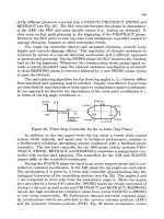
Fig. 3: Sharp edges experiment
(b)
(a)
Only the right bogie wheels climbed obstacle
(a). Then, the rover has been driven over
obstacle (b) (with an incident angle of
approximatively 20
◦
)
Fig. 4: Full 3D experiment
4 Wheel Slip Minimization
For wheeled rovers, the motion optimization is somewhat related to mini-
mizing wheel slip. Minimizing slip not only limits odometric error but also

increases the robot’s climbing performance and efficiency. In order to fulfill
this goal, several methods have been developed.
Methods derived from the Anti-lock Breaking System can be used for
rough terrain rovers. Because they adapt the wheel speeds when slip already
occurred, they are referred to as reactive approaches. A velocity synchroniza-
tion algorithm, which minimizes the effect of the wheels fighting each other,
has been implemented on the NASA FIDO rover [6]. The first step of the
method consists in detecting which of the wheels are deviating significantly
from the nominal velocity profile. Then a voting scheme is used to compute
the required velocity set point change for each individual wheel. However, per-
formance might be improved by considering the physical model of the rover
and wheel-soil interaction models for a specific type of soil. Thus, the traction
of each wheel is optimized considering the load distribution on the wheels and
the soil properties. Such approaches are referred to as predictive approaches.
In [7], wheel-slip limitation is obtained by minimizing the ratio T/N for
each wheel, where T is the traction force and N the normal force. Reference [8]
proposes a method minimizing slip ratios and thus avoid soil failure due to ex-
cessive traction. These physics-based controllers assume that the parameters
of the wheel-ground interaction models are known. However, these parameters
are difficult to estimate and are valid only for a specific type of soil and condi-
tion. Reference [9] proposes a method for estimating the soil parameters as the
534 P. Lamon and R. Siegwart
robot moves, but it is limited to a rigid wheel travelling through deformable
terrain. In practice, the rover wheels are subject to roll on different kind of
soils, whose parameters can change quickly. Thus, physics-based controllers
are sensitive to soil parameters variation and difficult to implement on real
rovers. In this section, a predictive approach considering the load distribu-
tion on the wheels and which does not require complex wheel-soil interaction
models is presented. More details about the controller can be found in [10].
Quasi-static model

The speed of an autonomous rover is limited in rough terrain because the nav-
igation algorithms are computationally expensive (limited processing power)
and for safety reasons. In this range of speeds, typically smaller than 20cm/s,
the dynamic forces might be neglected and a quasi-static model is appropri-
ate. To develop such a model, the mobility analysis of the rover’s mechanical
structure has to be done. It ensures to produce a consistent physical model
with the appropriate degrees of freedom at each joints. Then the forces are
introduced and the equilibrium equations are written for each part composing
the rover’s chassis. Because we have no interest in implicitly calculating the
internal forces of the system, it is possible to reduce this set of independent
equations. The variables of interest are the 3 ground contact forces on the
front and the back wheel, the 2 ground contact forces on each wheel of the
bogies and the 6 wheel torques. This makes 20 unknowns of interest and the
system can be reduced to 15 equations. This leads to the following equation
M
15x 20
· U
20x 1
= R
15x 1
(1)
where M is the model matrix depending on the geometric parameters and
the state of the robot, U a vector containing the unknowns and R a constant
vector. It is interesting to note that there are more unknowns than equations
in 1. That means that there is an infinite set of wheel-torques guaranteeing the
static equilibrium. This characteristic is used to control the traction of each
wheel and select, among all the possibilities, the set of torques minimizing
slip. The optimal torques are selected by minimizing the function
f = max(


i
T
i
/N
i
) i =1 6(2)
where T
i
and N
i
are thetractionand the normalforceapplied to wheel i .
Rover motion
Astatic model balances the forcesand momentsonasystem to remain at
rest or maintain aconstantspeed. Suchasystem is an ideal case and does not
include resistance to movement. Therefore,anadditional torque compensating
the
rolling
resistance
torque
mu
st
be
added
on
thew
heels
in
order
to
complete

3D Position Tracking in Challenging Terrain535
the model and guarantee motion at constant speed. This results in a quasi-
static model. Unlike the other approaches, we don’t use complex wheel-soils
interaction models. Instead, we introduce a global speed control loop, in order
to estimate the rolling resistance as the robot moves. The final controller,
minimizing wheel slip and including rolling resistance, is depicted in Fig. 5.
M
r
M
w
PID
d
V
+
−
M
c
r
V
Robot
Model &
s
Optimization
N
Distribution
Correction
+
+
o
M

V
d
desired rover velocity M
o
vector of optimal torques
V
r
measured rover velocity N vector of normal forces
M
r
rolling resistance torque s rover state
M
c
correction torque M
w
vector of wheel correction torques
Fig. 5: Rover motion control loop.
The kernel of the control loop is a PID controller. It allows to estimate
the additional torque to apply to each wheel in order to reach the desired
rover’s velocity V
d
and thus, minimizes the error V
d
− V
r
. M
c
is actually an
estimate of the global rolling resistance torque M
r

, which is considered as
a perturbation by the PID controller. The rejection of the perturbation is
guaranteed by the integral term I of the PID. We assume that the rolling
resistance is proportional to the normal force, thus the individual corrections
for the wheels are calculated by
M
w
i
=
N
i
N
m
· M
c
(3)
where N
i
is the normalforceonwheel i and N
m
the average of all the
normal forces. The derivativeterm D of thePID allowstoaccountfor non
modeled dynamiceffects and helps to stabilizethe system. The parameters
estimation for the controller is not critical because we are more interested
in minimizing slip than in reaching thedesired velocityvery precisely. For
locomotion in rough terrain, aresidual error on the velocitycan be accepted
as longasslip is minimized.
Experimentalresults
Asimulationphase using Open Dynamics Engine
2

has been initiated in order
to
test
the
approac
ha
nd
ve
rify
the
theoreticalc
onceptsa
nd
assumptions.
The
2
this librarysimulates rigid bodydynamicsinthreedimensions, including ad-
vanced joint typesand collision detection with friction.
536 P. Lamon and R. Siegwart
simulation parameters have been set as close as possible to the real operation
conditions. However, the intent is not to get exact outputs but to compare dif-
ferent control strategies and detect/solve potential implementation problems.
In the experiments, wheel slip has been taken as the main benchmark and the
performance of our controller ( predictive) has been compared to the controller
presented in [6] ( reactive). The reactive controller implements speed control
(spd) for the wheels whereas torque control (trq) is used in our approach.
Three dimensional surfaces are used for the experiments (see Fig. 6). Be-
cause the trajectory of the rover depends on the control strategy, we consider
an experiment to be valid if the distance between the final positions of both
paths is smaller than 0 1 m (for a total distance of about 3 5 m ). This distance

is small enough to allow performance comparison. For all the valid experi-
ments, predictive control showed better performance than reactive control. In
some cases the rover was even unable to climb some obstacles and to reach
the final distance when driven using the reactive approach. It is interesting to
note that the slip signal is scaled down for each wheel when using predictive
control. Such behavior can be observed in Fig. 7: the peaks are generally at
the same places for both controllers but the amplitude is much smaller for the
reactive controller. Another interesting result is that the difference between
the two methods increases when the friction coefficient gets lower. In other
words, the advantage of using torque control becomes more and more inter-
esting as the soil gets more slippery. Such a controller improves the climbing
capabilities of the rover and limits wheel-slip, which in turn improves the
accuracy of odometry. This way, it contributes to better position tracking
in rough terrain. Furthermore, our approach can be adapted to any kind of
wheeled rover and the needed processing power remains relatively low, which
makes online computation feasible. Finally, the simulations show promising
results and the system is mature enough to be implemented on SOLERO for
real experiments.
Fig. 6: Simulation environment Fig. 7: Wheel slip
0
0.0002
0.0004
0.0006
0.0008
0.001
0 0.5 1 1.5 2 2.5 3 3.5
Wheel slip [m]
x [m]
Wheel slip (Experiment 2)
Front wheel slip (spd)

Front wheel slip (trq)
Rover total slip (spd, scaled)
Rover total slip (trq, scaled)
2, 4 predictive
1, 3 reactive
4
3
2
1
3
4
2
(scale factor 800)
1
3D Position Tracking in Challenging Terrain537
5 Sensor Fusion
In our approach an Extended Information Filter (EIF) is used to combine the
information acquired by the sensors. This formulation of the Kalman filter has
interesting features: its mathematical expression is well suited to implement a
distributed sensor fusion scheme and allows for easy extension of the system
in order to accommodate any number of sensors, of any kind. Fig. 8 depicts
the schematics of the sensor fusion process.
H
imu
R
imu
R
vme
H
vme

Next step
H
odo
R
odo
H
inc
R
inc
3D−ODO
VME
State UpdateState Prediction
INS
imu
inc
Fig. 8: Sensor fusion scheme
Sensor
mo
dels:
The
po
sition,
ve
lo
cit
ya
nd
attitude
can
be

computed
by
in
te-
grating the measurementacquired by the IMU.However, the accelerometers
and gyrosare influencedbybias errors. In order to limit an unbounded growth
of
the
error
of
in
tegrated
measuremen
ts,
we
ha
ve
in
tro
ducedb
iases
in
the
model for the gyros(b
ωx
,b
ωy
,b
ωz
)and the accelerometers ( b

ax
,b
ay
,b
az
).
Unlikethe roll and pitchangles, the rover’s heading is not periodically up-
dated
by
absoluted
ata.
Therefore,
in
order
to
limitt
he
error
gro
wth,
as
pe
cial
provision is included in the z-gyro model: amore accuratemodeling, incorpo-
rating the scaling error Δ
ωz
.
The
rob
ot

used
for
thisr
esearc
hi
sa
partially
skid-steered
ro
ve
ra
nd
the
natural and controlled motion is mainly in the forward direction. Thus, the
motion estimation errors due to wheel slip and wheel diameter variations have
mu
ch
more
effect
in
the
x-z
plane
of
the
ro
ve
rt
han
along

the
transv
ersal
direc-
tion y. Therefore, scaling errors Δ
ox
and Δ
oz
,modeling wheel slip and wheel
diameter change, have been introduced only for the xand z-axes. The error
model for the odometry is tedious to develop because the robot is subject to
driveacross various typesofterrains. In order to avoid terrain classification
and complexwheel soil interaction modeling, we set the variance of the odom-
etry as being proportionaltothe acceleration undergone by the rover. Indeed,
slip
mostly
oc
curs
in
rough
terrain,
when
negotiating
an
obstacle,
while
the
robot is subject to accelerations. Similarly,the variance for the yawangle has
been set proportional to the angular rate. More details about the models of
538 P. Lamon and R. Siegwart

the IMU and 3D-Odometry can be found in [11] and reference [12] presents
the error model associated to the estimations of VME.
State prediction model: The angular rates, biases, scaling errors and accelera-
tions are random processes which are affected by the motion commands of the
rover, time and other unmodeled parameters. However, they cannot be con-
sidered as pure white noise because they are highly time correlated. Instead,
they are modelled as first order Gauss-Markov processes. Such modeling of
the state transition allows to both consider the time correlation and to filter
noise of the signals.
Experimental results
In order to better illustrate how each sensor contributes to the pose estimation
and in which situation, the experiments have been divided into two parts. The
first part describes the results of sensor fusion using inertial sensor and 3D-
Odometry only, whereas the second part involves all the three sensors i.e.
3D-Odometry, inertial sensor and VME.
Inertial and 3D-Odometry: The experimental results show that the inertial
navigation system helps to correct odometric errors and significantly improves
the pose estimate. The main contributions occur locally when the robot over-
comes sharp-shaped obstacles (Fig. 9) and during asymmetric wheel slip.
The improvement brought by the sensor fusion becomes more and more pro-
nounced as the total path length increases. More results are presented in [11].
d
c
True final height
Fig. 9: Sensor fusion with 3D-Odometry and inertial sensors. The ellipses emphasis
local corrections of the z coordinate.
Enhancement with VME: In theprevious tests, only proprioceptivesensors
have been integrated to estimate the robots position. Even if the inertial sensor
helps
to

correct
od
ometrice
rror,
there
are
situationsw
here
this
com
bination
of
3D Position Tracking in Challenging Terrain539
sensors does not provide enough information. For example, the situation where
all the wheels are slipping is not detected by the system. In this case, only
the odometric information is integrated, which produces erroneous position
estimates. Thus, in order to increase the robustness of the localization and to
limit the error growth, it is necessary to incorporate exteroceptive sensors. In
this application, we use visual motion estimation based on stereovision[12].
0
0.05
0.1
0.15
0.2
0.25
0.2 0.3 0.4 0.5 0.6 0.7 0.8 0.9 1 1.1
z [m]
x [m]
X-Z trajectories
VME

3D-Odometry
Estimated
Reference
Zone AZone BZone C
1
3
4
4
1
2
3
2
Fig. 10: Sensor fusion using 3D-Odometry, IMU and VME
In general, VME produces better estimates than the other sensors (but
at a much slower rate). In particular, its estimates allow to correct the ac-
cumulated error due to wheel slip between two updates. However, in zone C
(Fig. 10), less than thirty features have been matched between three subse-
quent images. The difficulty to find matches between these images is due to
a high discrepancy between the views: when the rear wheel finally climbs the
obstacle, it causes the rover to tilt forward rapidly. As a consequence, VME
provided bad motion estimates with a high uncertainty. In this situation, less
weight is given to VME and the sensor fusion could perfectly filter this bad
information to produce a reasonably good estimate using 3D-Odometry and
IMU instead. Finally, the estimated final position is very close to the mea-
sured final position. A final error of four millimeters for a trajectory longer
than one meter (0. 4%) is very satisfactory, given the difficulty of the terrain.
6 Conclusion
This paper showed how 3D position tracking in rough terrain can be im-
proved by considering the specificities of the vehicle used for locomotion.
3D-Odometry produces much better estimates than the standard approach

because it takes the kinematics of the rover into account. Similarly, by con-
sidering a physical model of the chassis it is possible to minimize wheel-slip,
540 P. Lamon and R. Siegwart
which in turn contributes towards better localization. In rough terrain, the
controller presented in Sect. 4 performs better than a controller based on a
reactive approach. Finally, experimental results of sensor fusion involving 3D-
Odometry, inertial sensors and visual motion estimation have been presented.
They prove that the use of complementary sensors improves the accuracy and
the robustness of the motion estimation. In particular, the system was able
to properly discard inaccurate visual motion information.
References
1. StrelowD,Singh S(2003) Online Motion Estimation from Image and Iner-
tial Measurements, The 11th International Conference on Advanced Robotics,
Po
rtugal
2. Nebot E, Sukkarieh S, Durrant-Whyte H(1997) Inertial navigation aided with
GPS
information,I
nt
he
pro
ceedings
of
the
Fo
urthA
nn
ual
Conference
of

Mechatronics and Machine Vision in Practice
3.
Siegw
art
R,
Lamon
P,
Estier
T,
Lauria
M,
Piguet
R(
2000)
Inno
va
tiv
ed
esign
for wheeled locomotioninrough terrain, Journal of Robotics and Autonomous
Systems, Elsevier,vol 40/2-3 p151-162
4. Lacroix
S,
MalletA
,B
onnafous
D,
Bauzil
G,
Fleury

S,
Herrb
M,
ChatilaR
(2002) Autonomousrovernavigationonunknown terrains: functions and inte-
gration,
In
ternational
Journal
of
Rob
otics
Researc
h
5. Lamon P, Siegwart R(2003) 3D-Odometry for rough terrain-Towards real
3D
na
vigation,
IEEE
In
ternationalC
onference
on
Rob
otics
and
Automation,
Taipei, Taiwan
6. Baumgartner E.T, Aghazarian H, Trebi-OllennuA,Huntsberger T.L, Garrett
M.S (2000) State Estimation and VehicleLocalization for the FIDO Rover,

Sensor Fusion and Decentralized Control in AutonomousRobotic Systems III,
SPIE Proc.Vol. 4196, Boston, USA
7. IagnemmaK,Dubowsky S(2000) Mobile robot rough-terraincontrol (RTC)
Forplanetary exploration,ProceedingsASME DesignEngineering Technical
Conferences, Baltimore, Maryland, USA
8.
YoshidaK,Hamano H, WatanabeT(2002) Slip-Based Traction Control of a
Planetary Rover, In theproceedingsofthe 8th International Symposium on
Experimental Robotics,ISER, Italy
9. Iagnemma K, ShibleyH,Dubowsky S(2002) On-Line TerrainParameterEsti-
mationfor Planetary Rovers, IEEE InternationalConference on Robotics and
Automation, WashingtonD.C, USA
10.
Lamon P, Siegwart R(2005) Wheel torque control in rough terrain-modeling
and simulation, IEEE International Conference on Robotics and Automation,
Barcelona,
Spain,
in
press
11.
Lamon P, Siegwart R(2004) Inertial and 3D-odometry fusion in rough terrain
To
wa
rds
real
3D
na
vigation,
IEEE/RSJI
nt

ernationalC
onference
on
In
telligent
Robots and Systems, Sendai, Japan
12. Jung I-K, Lacroix S(2003) Simultaneous Localization and Mapping withStere-
ovision, International Symposium on Robotics Research, Siena
Efficient Braking Model for Off-Road Mobile
Robots
Mihail Pivtoraiko, Alonzo Kelly, and Peter Rander
Robotics Institute, Carnegie Mellon University
, ,
Summary. In the near future, off-road mobile robots will feature high levels of
autonomy which will render them useful for a variety of tasks on Earth and other
planets. Many terrestrial applications have a special demand for robots to possess
similar qualities to human-driven machines: high speed and maneuverability. Meet-
ing these requirements in the design of autonomous robots is a very hard problem,
partially due to the difficulty of characterizing the natural terrain that the vehicle
will encounter and estimating the effect of these interactions on the vehicle. Here
we present a dynamic traction model that describes vehicle braking on a variety of
terrestrial soil types and in a wide range of natural landscapes and vehicle velocities.
This model was developed empirically, it is simple yet accurate and can be readily
used to improve model-predictive planning and control. The model encapsulates the
specifics of wheel-terrain interaction, offers a good compromise between accuracy
and real-time computational efficiency, and allows straight-forward consideration of
vehicle dynamics.
Keywords: Modeling dynamics off-road robotics
1Introduction
As developing autonomousoff-road vehicle technology allows robots to travel

at higher speed and negotiaterugged terrain, vehicle modelingbecomes in-
creasingly relevantfor motion planningand control. An efficientbrakingtrac-
tion modelcan greatlyenhance vehicle autonomy by addressing two keyprob-
lems:itcan determine whether thepath ahead,given its slope and ground
characteristics, presentsrisks suchastip-over, and provideapreciseestimate
of the stoppingdistance. Precisionofthe model is very important,but it
shouldalso be very efficientcomputationally because it hastobecontinually
evaluated if it is usedfor control or tightlycoupledwith the path planning
algorithm.Certainly, agrossover-estimation for the problems above willlikely
keep the vehicle safe, howeverincluttered naturalterrain suchapproachwill
P. Corke and S. Sukkarieh (Eds.): Field and Service Robotics, STAR 25, pp. 541–552, 2006.
© Springer-Verlag Berlin Heidelberg 2006
542 M. Pivtoraiko, A. Kelly, and P. Rander
either result in slow, inefficient traversal, or may cause a failure of the path
planner to generate an admissible path.
1.1 Prior Work
Great overviews of automobile off-road mobility and approaches to soil mod-
eling are presented in [1]. Quite a few fairly detailed models of the wheel-soil
interaction were proposed specifically for motion planning applications. For
example, [7] and [11] present approaches that model the soil as a mass-spring
system. These models provide fairly good results in describing compression,
shear and plastic deformations in soils. However, such approaches are yet to
be thoroughly validated experimentally. Moreover, the reported run-times of
these modeling methods do not appear to be fast enough to render them fea-
sible in real-time robot control scenarios. The approaches that were shown to
be suited for controlling mobile robots tend to circumvent the issue of com-
putational efficiency by further simplification. Often the Coulomb principle of
friction, or its derivative is used to estimate the amount of rolling friction that
the vehicle experiences [8]. Several parameters of the terrain are used in [10]
to estimate normal and lateral tangential forces at the wheel contact patch.

A similar approach to traction modeling that can also be adapted on-line was
presented in [9]. That work is focused on planetary applications with accom-
panying quasi-static assumptions. It is also assumed that the wheels are rigid.
Pneumatic tires used for terrestrial applications, however, are elastic. Mor-
ever, in off-road applications the inflation pressure is typically lower in order
to avoid rigid-mode operation that may cause excessive compaction of soil
[1]. In off-road robotics it is still common to ignore these effects and consider
wheels to be rigid, or simplify even further by using Coulomb friction. We
show that at higher speeds and rough terrain, such methods result in grave
errors in characterizing braking (e.g. stopping distance). Our approach, how-
ever, is as efficient as these approximations employed in the field, but offers
much better accuracy, especially at higher speeds.
1.2 A New Approach
We conducted a significant field experimentation effort with autonomous off-
road robots, and this prompted an empirical approach to capturing the com-
plexities of wheel-terrain dynamics in natural environments (Fig. 1). An initial
observation was that it was generally not possible to consider the net braking
force of the vehicle (with gravity effects removed) to be some constant value.
In fact, in some cases on soft soil the net braking force on a slope was off by as
much as 50% from its value on level ground. Depending on vehicle dynamics,
this can result in a miscalculation of the stopping distance by several meters,
which may be a serious error when operating in cluttered natural terrain.
We propose an approach that provides accurate estimates of tractive brak-
ing force and involves a simple and efficient model of several parameters. The
Efficient Braking Model for Off-Road Mobile Robots 543
values of the parameters are determined experimentally by measuring the
deceleration during vehicle braking and combining these measurements with
vehicle state information. This “training” procedure can be easily done in the
field, and even autonomously by the robot. For example, every time the robot
has to stop, it can verify its braking model. In this manner, the model can be

refined on-line and adapted as the robot moves into different type of terrain.
This formulation of the model was shown to work well on off-road robots op-
erating on a wide variety of terrain types, such as clay, soil with sod cover,
gravel, coarse sands, and packed snow, as well as at various speeds and on
natural slopes (typical to mid-West region, the plains and the desert).
This model can be used in model-predictive control to estimate the stop-
ping path [12], the guaranteed stopping distance that is necessary for vehicle
safety, which is mainly a function of a complex relationship between vehicle
speed, tire-ground interface, and terrain slope. The model can also be utilized
by the path planning algorithm to generate plans that respect this stopping
path. Since the present model estimates major forces acting on the vehicle
during braking maneuvers, it can also be used in kinodynamic motion plan-
ning approaches. Moreover, if an estimate of tire sliding friction coefficient
is available, then this model can predict whether robot’s wheels are going to
lock up (which generally must be avoided [4]).
2Experimental Procedure
In thissection we givethe details of experiments thatpromptedustoformu-
latethis model of braking. In our experiments, aterrain patch thatisagood
representativeofthe overall terrain is chosen (oftennatural environments have
fairly uniform type of ground overlarge areas: meadows, field, desert, etc.).
The vehicleacceleratestoacertainvalueofvelocity, v
i
,and thenapplies the
brakeswithsome knownforce(either maximum application for vehiclesthat
have no brakingforcefeedback, or acertain knownvaluefor those that do).
544 M. Pivtoraiko, A. Kelly, and P. Rander
Most vehicle control systems with closed-loop velocity control estimate veloc-
ity more frequently than it can significantly change, so it is possible to achieve
the temporal resolution sufficient to obtain the velocity profile of vehicle stop-
ping. The velocity data can be plotted against time as in Fig. 2. Note that

actual velocity in the plot goes slightly negative after reaching zero. This is
due to expansion of suspension springs that were compressed during braking.
The time when braking was initiated (when desired velocity is set to zero)
is recorded, along with the time when the actual velocity reached zero, t
f
.
The average value of deceleration in a particular experiment is estimated as
shown in (1).
¯
a
x
=
v
t
t
f
− t
i
(1)
The value ¯a
x
is the slope of thevelocitydrop in the figure.Inthis calcu-
lation, it is importanttonote that, as can be seen in Fig. 2, there is acertain
delayafter the system commands azero velocitytowhen the velocityactually
beginstodrop. This delayofpropagation of the command, t
delay
,depends
solelyonhardware. It wasonaverage300 ms. on our robots. Forbraking
at higher speeds, it is much less thanoverall Δt,yet needs to be taken into
account. Therefore, we take t

i
as time of zero-velocitycommandplus t
delay
,
and sample v
i
specificallyatthat value of t
i
to obtain an accurate estimate
of the slope.
Throughout ourexperiments we made sure that thedegree of brakeen-
gagement wasconstant. In particular, we were interested in maximumbraking,
i.e. in engagingthe brakes completely.
The same experiment wasthen repeatedwith variousvehicle velocities and
on the ground of variousslopes and terrain types. We fitted the above data
gatheringprocedure in the robots’ controller code, so that we couldobtain
adata pointatany time whenthe robot made astop.Inthis manner we
obtained thedata overseveralmonths as therobots were usedfor avariety
of navigation and perception experimentsonthe PerceptORprogram.Thus
we obtained thousands of datapoints thatwere then analysed.
If we plot the measurements of decelerations versus slope for achoice
of terrainand subtractthe effects of gravity,wesee that theresulting net
brakingforceslightly increases with the increase of slope angle.Anexample
plot is presented in Fig.3,whichshows the normalized braking force, aratio
of thenet breaking force to vehicle weight F
b
/W ,asafunction of slopeand
velocity. The dependence of deceleration on initial velocityisalso noticeable,
albeit not as pronounced. Interestingly,these datapoints exhibitproportional
dependence of normalizedbraking force on slopeangle. Hence, asingle linear

model should be abletopredict the braking force for both downhilland uphill
braking maneuvers.
Note, however, that ourobservations have been made in tests on slopes
well within limitsofvehicle traversability, whichwas about 17 degree slopes
Efficient Braking Model for Off-Road Mobile Robots 545
forour hardware. It is naturaltoexpect that beyond this range of slope values
the dependence is no longer linear.
3DiscussionofResults
In this section we developthe necessary concepts to understandthe factors
influencingtraction duringvehicle braking. We then use the developedcon-
cepts in an effort to explain our experimental observationsand suggest amodel
based on this analysis.
3.1 Vehicle Force Balance
As astarting point, we developthe force analysis of the vehicleduring braking.
Among the importantnotions that we discuss hereare normal forces on tires,
pressureofthe tire contact patch, and the dynamic load transfer.
During braking, the major forces acting on the vehicle are related through:
F
b
= W
a
x
g
− W sin θ (2)
Here F
b
is the net brakingforce, g is accelerationdue to gravity, a
x
is
brakingdeceleration, W = m

veh
g is vehicle weight, and θ is the terrain slope
angle(here we considerdownhill slopesasnegative, and uphill as positive).
Thefirst term on the rightside of (2) is the d’Alembert force [2] (see Fig.4).
546 M. Pivtoraiko, A. Kelly, and P. Rander
Given thatthe vehiclecenter of gravity,(x
cg
,y
cg
,z
cg
), is known, we can
express the sum of torquesaround thecontactpointoffrontwheels(for
downhill slopes, assumingpositive torque is clockwise):
− ( L
wb
− x
cg
) W cos θ + W
r
L
wb
+ z
cg
W
a
g
+ z
cg
W sin θ =0 (3)

Here L
wb
is wheel base, and W
r
is weightonthe rear axle. When the
vehicle is stationaryonlevel ground, the loadsonfrontaxle, W
f
,and rear
axle, W
r
,are determined by:
W
f
= W
L
wb
− x
cg
L
wb
; W
r
= W
x
cg
L
wb
(4)
In case of avehicle decelerating on aslope, we obtain thenormal forces
on rear and frontwheels by summing the torques aroundfront and rear wheel

contactpoints, respectively:
W
f
=
W
L
wb
( x
cg
cos θ + x
cg
sin θ + z
cg
a
x
g
)(5)
W
r
=
W
L
wb
((L
wb
− x
cg
)cos θ − z
cg
sin(− θ ) − z

cg
a
x
g
)
We observefrom (5) that duringbrakingdownhill, there is asignificant
dynamicloadshift fromreartofrontaxles.Note that W
r
waswritten with
the z
cg
sin(− θ )term to underscore thefact that for downhillslopes θ<0.
We considerpressure on the tire contact patchfor frontand rear wheels
as the ratio of axle load to contact area. The vehicles we had availablefor
experiments in this study had dual rear tires, so we estimate thatthe pressure
of front tires’ground contact wastwice thatofreartires for thesame normal
load.
Efficient Braking Model for Off-Road Mobile Robots 547
3.2 Braking Force
We consider that the braking torque results in a longitudinal force F
h
at
the wheel-terrain interface. Since the goal of this work was to understand
the effects of maximum braking that determines minimum allowable stopping
distance and outlines the upper bound on dynamics effects due to braking,
we understand that F
h
represents full engagement of the brakes and depends
solely on braking hardware, hence always constant. Here we also assume that
braking happens on a straight path. We visualize the effect of this force in the

detail of interaction of an off-road tire with terrain in Fig. 5.
The hardware braking force F
h
is counter-acted by the terrain acting on
tire tread. If the magnitude of this force exceeds the shear strength of the
terrain, it will no longer be able to resist this shear force, and the wheel will
skid.
The other force in the tire-ground interface that was found to have sig-
nificant effect on braking is rolling resistance R
x
. This resistance is always
present, and in the case of pneumatic tires its value is determined by many
factors, such as tire material and design, temperature, vibration, pressure
of the ground contact patch (normal force on the tire). Terrain compaction
(related to pressure of the patch) and bulldozing effects in soft soil are also
important contributing factors to this resistance [1]. While F
h
can be con-
sidered constant for a given vehicle, estimating R
x
is complicated due to the
variety of factors influencing it.
Through experimentation we found that we can approximate all longitu-
dinal forces acting on the vehicle during braking by lumping them into the
sum of the force due to the torque supplied by the braking hardware, and the
rolling resistance. Then, the overall braking force is considered to be:
F
b
= F
h

+ R
x
(6)
The key to accurately predicting the braking force is estimating rolling
resistance R
x
.
In our experiments it was also determined that out of all factors influencing
rolling resistance, the most significant one is the pressure at ground contact.
A lesser, but noticeable, effect has vehicle speed. In the following two sections
we explain these two factors.
548 M. Pivtoraiko, A. Kelly, and P. Rander
3.3 Effect of Terrain Slope
It is important to consider contact pressure here because in general rolling
resistance is roughly proportional to this pressure (although this relationship
is complex and highly non-linear) [1].
For the case of level ground we can decompose (6) into the contributions
of front and rear wheels:
F
b
= 2 F
h
+ R
xr
+ R
xf
Here F
h
is the same for front and rear wheels since our vehicles had the
interlocked differential. Also our robots had dual rear tires, which resulted in

twice the contact area and half the ground contact pressure for rear tires than
for the front tires. Hence, let us suppose (only for clarification purposes in this
section) that due to the difference in contact pressures, the rolling resistance
values can be related through R
xf
= 2 R
xr
.
As was shown earlier, during downhill braking there is a significant dy-
namic load shift to front wheels, W
r
< W
f
. Because of this the pressure
developed at front wheel contact point greatly exceeds that at rear wheel
contact, and even more so in the case of rear dual tires. R
xf
increases dra-
matically, more than R
xr
decreases (in part due to half the contact pressure).
The overall value of F
b
becomes greater than on level ground.
During braking uphill, similar issues come into play. However, in this case
the load shift to front axle is less significant (see (5)), in fact even less than
on level ground due to x
cg
sin θ term. In this case W
r

> W
f
, whereas for level
ground we had W
r
= W
f
. However, since rear tires have nearly “half the
effect” on rolling resistance than the front tires, the overall braking force is
less than on level ground.
3.4 Effect of Velocity
Among the factors influencing rolling resistance is vehicle velocity [2]. The
rolling resistance is directly proportional to velocity because of increased tire
deformation work and vibration in the tire. The influence of velocity becomes
more significant when tires with lower inflation pressures are used, as is often
the case for off-road vehicles. Lower tire pressure is used to allow tires to be
more elastic, since the work required for flexing the tire is much less than the
work of compacting and bulldozing soft soil. Greater elasticity, however, causes
greater hysteresis losses with increasing vehicle velocity. The effect of velocity
on rolling resistance was found to be less significant, but still noticeable.
4Derivingthe Model
In this section we combineour experimental observationswith the insights
developed above to formulate ourmodel of braking force. We describe how
Efficient Braking Model for Off-Road Mobile Robots 549
this model could be easily adapted online and discuss the results of validating
the model through experiments with robots.
4.1 Formulating the Model
As we discussed, the results of our experiments prompted us to make a sim-
plifying assumption that within the range of slope values that the vehicle can
safely handle, the braking force is proportional to the slope.

The essence of our model is stated as:
• The braking force (without gravity effects) can be approximated well by
a linear model:
∂F
b
∂θ
= m
where θ is groundslopeangle and m is acoefficient.Wecan fit aline
F
b
= mθ + b to the test data in the least-squaresmanner and use it to
obtain future estimatesof F
b
based on slope.
• The coefficients m and b above alsoexhibits lineardependence on initial
velocityofthe vehicle (right before braking is initiated):
∂m
∂v
i
= m
m
;
∂b
∂v
i
= m
b
Thus, the overallmodel containsonly four parameters: m
m
, m

b
, b
m
, b
b
:
m ( v
i
)=m
m
v
i
+ b
m
; b ( v
i
)=m
b
v
i
+ b
b
(7)
So that
F
b
= m ( v
i
) θ + b ( v
i

)(8)
We again underscorethat the developmentofthe model wasbased on ex-
perimental data, which wasavailable for arange of terrain sloperoughly from
− 15
◦
to 15
◦
.Whilethis model cannotbeextrapolated outsidethe experimen-
tal range in which it wasdefined, we can reasonabout thecharacterof F
b
outside of this range. In particular, basedonprevious discussion, we estimate
thatfor greater uphill slopes, the effect of rolling resistance will diminish due
to decreasingnormal force, i.e. contact pressure, and F
b
willapproach F
h
(omitting gravityeffects, as usual). At acertainpointthe slope becomesun-
safe, whenthe shear capacityofthe wheel-terrain interface becomes equal
to F
h
.For steeper downhillslopes similararguments apply: rolling resistance
will become less dominantwith decreasingsoil contact pressure, and at some
pointthe shearcapabilitymay no longer support the vehicle.
In theexperiments thatlead to formulation of this model, we have assumed
that thedegree of application of the brakes wasconstantthroughout the
experiments (e.g.for emergency braking, whichoften determines thelook-
ahead distance for apath planner,maximumactuator powerisused). For
550 M. Pivtoraiko, A. Kelly, and P. Rander
other actuator modes this model is also applicable, but additional coefficients
may be necessary to allow for other than maximum braking (e.g. slight, half

way, etc.). On the other hand, the benefits of this expression of the model
are that it is very simple and intuitive, quite easy to adjust, yet powerful
enough to account for peculiarities of braking hardware and ground types,
while requiring very low online computational overhead.
4.2 Experimental Results
As we saw in the previous section, the key result of the model, F
b
, is obtained
simply by evaluating three linear equations (8). Thus, its computational cost
is minimal and comparable to the fastest approximations used in the field
(e.g. using simple Coulomb friction equations). Such methods, however, do
not consider the dependence of braking on changes in wheel-terrain interface
due to velocity and slope, and thereby result in large errors. The PerceptOR
robots previously used similar methods to estimate stopping distance, and it
was routinely over-estimated with error on the order of 50% (stopping distance
estimates lower than the actual value must be avoided, as they may lead to
collision).
Our model was verified through a series of experiments: braking on level
ground, downhill and uphill, at velocities ranging from 1 to 4 m/s, and with
10 repetitions of each test to ensure correlation (variability of measurents
was less than 5%). Figure 6 a) shows the results of 200 such experiments
(the horizontal axis represents test number), where the stopping distance was
estimated using the model (as discussed in Section 5.1) and compared to
actual measurements. Given predicted and actual values of stopping distance,
statistical analysis was performed on the error of this braking model. Figure
6 b) presents the plot of mean values of this error as a function of vehicle
velocity (before braking). Note that the model always slightly over-estimates