Field and Service Robotics - Corke P. and Sukkarieh S.(Eds) Part 13 pps
Bạn đang xem bản rút gọn của tài liệu. Xem và tải ngay bản đầy đủ của tài liệu tại đây (2.9 MB, 40 trang )
486 T.M. Howard and A. Kelly
4.1 Rocky 7 Rate Kinematics, Actuator Dynamics, and Wheel Slip
The Rocky 7 rover has eight actuators: a steering actuator on each of the
front two wheels and six drivable wheels. In order to get a realistic model of
actuator dynamics, a first-order lag was assumed.
v
c
out
( t )=
α
1
dt
τ
[ v
c
in
( t ) − v
c
out
( t − τ )] + v
c
out
( t − τ )(17)
ψ
1 , 2
out
( t )=
α
2
dt
τ
[ ψ
1 , 2
in
( t ) − ψ
1 , 2
out
( t − τ )] + ψ
1 , 2
out
( t − τ )(18)
Thewheelslip model assumes that only afractionofthe requestedvelocityis
achieved. Inverse rate kinematics generate theachieved V
out
, Ω
out
due to the
actuatordynamics and wheel slip model.
4.2 Rocky7Suspension Kinematics
Just as in the general solution, the suspension model provides amapping
of thelinear and angular velocities estimated by the actuatordynamics and
wheel slip models from the body frame to the world frame,except nowthe sus-
pension model is known. Taking advantageofthe fact thatthere aresix con-
trols (attitude(φ , θ ), altitude ( z ), and the three rocker-bogie angles(ρ , β
1
, β
2
))
and six constraints ( z
c
1
- z
c
6
), the same numerical methodused in the inverse
trajectory generation solverisapplied. An errorvector ∆z
=[∆z
c
1
, ···, ∆z
c
6
]
T
is formed from the difference between the elevationofthe terrain andthe
contact pointofeachofthe sixwheels.The initial guessofcontrol is adju-
sted by the product of theinverse Jacobianofthe forwardkinematics of the
contact points with respect to the world frame andthe elevation errorvector
untilthe terminalconditions aremet.
4.3 Rocky7Kinetic Motion Model
Since the Rocky7roverisaterrain-following mobile robot, the kinetic model
follows the form of equation (13). The attitude and altitude are determined
from the suspension model for agiven pose.
4.4 Rocky7TrajectoryKinematics
The forward model of trajectory generationfor theRocky 7roverisgenerated
by
integrating equation (13).
Trajectory Generation on Rough Terrain Considering Actuator Dynamics487
5 Implementation
5.1 Forward Solution of Trajectory Kinematics
In order to determine the terminal pose ( x
f
, y
f
, ψ
f
) of the rover, the system
dynamics described in equations (14)-(16) must be integrated with respect to
time. These state equations are coupled and nonlinear. We have found simple
Euler integration to be sufficient:
x
t + ∆t
= x
t
+ v
x
out
t + ∆t
cos( θ ( x
t
,y
t
,ψ
t
))cos ( ψ
t
) ∆t (19)
y
t + ∆t
= y
t
+ v
x
out
t + ∆t
cos( θ ( x
t
,y
t
,ψ
t
))sin ( ψ
t
) ∆t (20)
ψ
t + ∆t
= ψ
t
+
cos( φ ( x
t
,y
t
,ψ
t
))
cos ( θ ( x
t
,y
t
,ψ
t
))
ω
z
out
t + ∆t
∆t (21)
ω
z
out
t + ∆t
= f ( ω
z
in
t + ∆t
)(22)
v
x
out
t + ∆t
= g ( v
x
in
t + ∆t
)(23)
Noticethatthe output linearand angular velocities of the rate kinematics are
used
in
this mo
del. In
th
is
metho
d,
ac
onfiguration
at
eac
hn
ew
po
se
mu
st
be
found. The algorithm canbespedupdramaticallybyusing theprevious con-
figuration at time t − ∆t as the seed for the configurationatthe current time t .
It is essential that ∆t be small enough to accurately model the integral of
the system dynamics and capturethe terrain alongthe path. Forexample,
in
tra
jectory
generation
ove
rt
he
scale
of
af
ew
ro
ve
rl
engths,
12-15
iterations
maybeenoughtoaccurately model the system dynamics butthesemay still
miss small terrain disturbances that mayinfluencethe path enoughtomatter.
5.2
Tr
aj
ectory
Generation
Using
In
ve
rse
Tr
aj
ectory
Kinematics
Utilizing the forward model of trajectory kinematics developed in the pre-
vious section, along with the controls and methods of section 3.1 and 3.2,an
inverse trajectory kinematics solverwhichaccounts for both rough terrain and
actuatordynamics is obtained.
5.3 Initialization/Termination
Sincethe numerical methodused in this work does notguarantee global con-
vergence, aheuristic whichplaces the terminal posture of theinitialguess
nearthe goal postureisrequired. It wasfound thatthe solutiontothe two-
dimensionalt
ra
jectory
generation
problemp
laces
the
terminal
po
sture
of
the
initial guess within 15%ofthe goal on avariety of interesting terrains.This
is close enough to ensure convergenceinmost applications. In thecase of
488 T.M. Howard and A. Kelly
an exceptional terrain disturbance which incurs a large terminal posture per-
turbation, line searches or scaling of the change of parameters ( ∆p) can be
implemented to prevent overshoot and divergence from the solution.
The set of termination conditions used for the trajectory generation algo-
rithm were similar to those in [1], stopping iterations when [ ∆x
f
, ∆y
f
, ∆ψ
f
,
∆ω
f
]
T
=[0. 001m , 0 . 001m , 0 . 01rad , 0 . 01
rad
sec
]
T
.Likewise, the suspension model
required millimeter residuals in ∆z
c
i
.
6R
esults
6.1 Rough TerrainTrajectoryGeneration Example
This section demonstrates the need of rough terrain trajectory generation
by examining an example situation. In this example, the Rocky7platform is
asked to findacontinuous trajectory between two postures as seen in Figure4.
The relativeterminal posture[x
f
, y
f
, ψ
f
, ω
f
]
T
is equal to [3. 0 m ,5. 0 m ,
π
2 . 0
ra
d
,
0 . 0
rad
sec
]
T
.Inorder to isolatethe effectofneglecting the influence of attitude
in the trajectory generator, rate kinematics are ignored in this example.
Fig. 4. Example Rough Trajectory Generation: This figure shows an example tra-
jectory generation problem, where a continuous path is desired between an initial
posture inside a crater and the final posture just over the lip of the crater.
First,the two-dimensional continuous curvaturepath is solvedtomillime-
ter accuracy and fed into the three-dimensional forward solution. The two-
dimensionalsolution incurs aterminal position error of 6.2%(45.3cm) of the
entire arclength of the solution. The three-dimensional trajectory generator
finds anew path that is continuous in angular velocity, with an initial and
final velocityof1m/sec, formilimeter accuracy in only 3iterations. Figure
5shows the difference between the two-dimensional system model and three-
dimensional system
mo
del
paths
and
ho
wt
he
latter
generatest
he
correct
trajectory.
Trajectory Generation on Rough Terrain Considering Actuator Dynamics489
Fig. 5. Trajectory Generation Solution: This figure shows the result of neglecting
attitude in the forward model (two-dimensional solution) and the new solution
based on a three-dimensional system model. By neglecting attitude, the terminal
position is off by 6.2% when compared to the total arclength of the solution.
6.2 General Results
To
ev
aluate
the
need,p
erformance,
and
be
ha
vior
of
this
algorithm,
seve
ral
thousand tests were run to understand ratesofconvergenceand rangeof
errors to expect. One behavior that wasrecognized is that even though error
would increase dramaticallywith rougher terrain, the number of iterations
required to meet the terminationconditions did not. The numerical method
that we areusing attempts to remove all errorinasingle iteration, so this
behavior suggests that thefirst order approximation is agood one.
7C
onclusions
In the context of mobile robots whichmust alreadyexpend significanteffort
to understand terrain complexity, the use of aflat terrain assumptionintra-
jectory generation is difficulttojustify.However, as thepaper hasshown, the
use of terrain information requiresacertain amountofeffort to develop a
more complex generation algorithm. While space wasnot available to address
acomputation comparison,the additionalcomputation for3Dmodels is not
as
ignificantfactor in practice.
Avery general algorithm has been presented whichcan generate conti-
nuouspathsfor mobilerobots obliged to driveoverrough terrain while subject
to additional nonidealities suchaswheelslip and actuatordelays. The essen-
tial problem is to invert amodel of howparameterized controlinputs,terrain
shap
e,
terrain
in
teractiona
nd
actuatord
ynamic
mo
dels
determine
the
termi-
nal state of avehicle at all futuretimes. Anumerical technique wasadopted
due to the assumedinabilitytoexpress terrain shapeinclosed form. However,
once anumerical approachisadopted, it alsomeans that anyforward model
490 T.M. Howard and A. Kelly
can be inverted to produce continuous controls subject only to the capacity
of the numerical linearization to converge. In principle, a full Lagrangian dy-
namics model can be inverted using our technique, for example.
The Rocky 7 prototype rover was used to illustrate the application of
the general models of suspension and rate kinematics to a specific robot. For
any vehicle, only forward rate kinematics and forward suspension models are
needed to use the rest of the algorithm. Our results suggest there is much to
gain and little to lose by moving to fully 3D models. Such predictive models
lead to improved performance by removing as much model error as possible at
planning time — so that path following controls are used only to compensate
for truly unpredictable disturbances.
While the algorithm has been presented in the context of planning com-
putations, it promises to be equally valuable for the generation of corrective
trajectories in feedback path following controls. Future work will assess the
value of the algorithms for this purpose in the hope of developing short term
path followers which maximally exploit the model and terrain information
which can be assumed to be present in most present and future mobile ro-
bots.
Acknowledgment
This research was conducted at the Robotics Institute of CMU under contract
to NASA/JPL as part of the Mars Technology Program.
References
1. Nagy, B., Kelly, A., ”Trajectory Generation for Car-Like Robots Using Cubic
Curvature Polynomials”, Field and Service Robots 2001 (FSR 01), Helsinki,
Finland - June 11, 2001.
2. Simeon, T., Dacre-Wright, B., ”A Practical Motion Planner for All-terrain Mo-
bile Robots”. 1993 IEEE/RSJ International Conference on Intelligent Robots
and Systems, Yokohama, Japan - July 26-30, 1993.
3. Iagnemma, K., Shibly, H., Rzepniewski, A., Dubowsky, S., ”Planning and Con-
trol Algorithms for Enhanced Rough-Terrain Rover Mobility”. International
Symposium on Artificial Intelligence and Robotics and Automation in Space
2001 (i-SAIRAS 01), St-Hubert, Quebec, Canada - June 18-22, 2001.
4. H Delingette, M. Herbert, and K Ikeuchi, ”Trajectory Generation with Cur-
vature Constraint based on Energy Minimization”, Proc, IROS, pp 206-211,
Osaka, Japan, 1991.
5. Shin, D.H., Singh, S., ”Path Generation for Robot Vehicles Using Composite
Clothoid Segments” tech. report CMU-RI-TR-90-31, Robotics Institute, Car-
negie Mellon University, December, 1990.
6. Tarokh, M., McDermott, G., Hung, J. ”Kinematics and Control of Rocky 7
Mars Rover.” Tech Report. August 1998.
7. Volpe, R., ”Navigation Results from Desert Field Tests of the Rocky 7 Mars
Rover Prototype.” International Journal of Robotics Research, 1998.
Results in Combined Route Traversal and
Collision Avoidance
Stephan Roth, Bradley Hamner, Sanjiv Singh, and Myung Hwangbo
Carnegie Mellon University. 5000 Forbes Ave., Pittsburgh, PA 15213, USA.
{ , ,,
}
Summary. This paper presents an outdoor mobile robot capable of high-speed
navigation in outdoor environments. Here we consider the problem of a robot that
has to follow a designated path at high speeds over undulating terrain. It must also
be perceptive and agile enough to avoid small obstacles. Collision avoidance is a key
problem and it is necessary to use sensing modalities that are able to operate robustly
in a wide variety of conditions. We report on the sensing and control necessary for
this application and the results obtained to date.
Keywords: Outdoor mobile robot, path following, collision avoidance
1I
nt
ro
duction
While the use of mobile robots in indoor environments is becoming common,
the outdoors stillpresentchallenges beyond the state of the art. This is be-
cause
the
en
vironmen
t(
we
ather,t
errain,
ligh
ting
conditions)
can
po
se
serious
issues in perception and control. Additionally,while indoor environments can
be instrumented to provide positioning, this is generally not possible outdoors
at
large
scale.
Ev
en
GPS
signals
are
degraded
in
the
presence
of
ve
getation,
builtstructures andterrain features. In the most general version of the prob-
lem, arobot is given coarselyspecified via points and must find its way to
the
goal
usingi
ts
ow
ns
ensors
and
an
yp
riori
information
ove
rn
atural
terrain.
Suchscenarios, relevantinplanetary explorationand military reconnaissance
are the most challenging because of the manyhazards –side slopes, negative
obstacles and obstacles hidden under vegetation –that must be detected. A
variantofthis problem is for arobot to followapath that is nominally clear
of obstacles but not guaranteed to be so. Suchacase is necessary for outdoor
patrolling applicationswhere amobile robot must traveloverpotentially great
distances
without
relying
on
structures
uc
ha
sb
eacons
and
lane
markings.
In
addition to avoiding obstacles, it is important thatthe vehicle stayonthe
designated route as much as possible.
P. Corke and S. Sukkarieh (Eds.): Field and Service Robotics, STAR 25, pp. 491–504, 2006.
© Springer-Verlag Berlin Heidelberg 2006
492 S. Roth et al.
Perception is typically the bottleneck in outdoor navigation, especially at
speeds higher than a few meters/sec. This is primarily because perception of
small obstacles (as small at 15 cm high) at or beyond the stopping distance
ahead of the robot is typically only possible using laser ranging. Laser ranging
produces detailed shape of the terrain but is limited in sampling and scanning
speed.
Here we report on the perception and guidance that we have developed for
an outdoor patrolling robot (Figure 1) that uses two low-cost laser scanners
to develop an understanding of the world around it. In specific, we report on
methods of obstacle detection and collision avoidance for this robot while it
travels at speeds at up to 5 m/s.
Fig. 1. Grizzlyisanavigationtest-bedbuilt upon acommercially available All
TerrainVehicle (ATV). It uses twolaserscanners to perceive the shapeofthe world.
The vehicleisequippedwith differential GPS and asix-axis inertial measurement
unit that providesaccurate attitude.
2Related Work
There has been agreat deal of attention paid to parts of the problem of au-
tonomouso
pe
ration
in
semi-structured
en
vironment
ss
uc
ha
si
np
orts[
6],
un-
derground mines [9], and highways[3]. In some of these cases, theenvironment
can be controlled enough that obstacle detection can be simplified to ensuring
that the machines are capable of stopping for peopleorvehiclesized obstacles.
Autonomous machines operating in natural environments, however, must be
abletodetect several differenttypes of obstaclesincluding side slopes and
negativeobstacles. This is accomplished by using sensors that can determine
the
shap
eo
ft
he
wo
rld
around
them.
Stereo
vision
[11],
colors
egmen
tation
[1], radar [8] and laser range finders [5] have all been used for obstacle detec-
tion. Unfortunately,passive visionsuffers from lighting, color constancy, and
Results in Combined Route Traversal and Collision Avoidance 493
dynamic range effects that cause false positives and false negatives. Radar is
good for large obstacles, but localization is an issue due to wide beam widths.
Single axis laser scanners only provide information in one direction, and can
be confounded by unmeasured pitching motion and mis-registration. Two axis
scanners are also used, which provide more information, but are very costly.
Several systems have demonstrated off road navigation. The Demo III
XUV drives off-road and reaches speeds up to 10 meters per second. The
speeds are high, but the testing environments are rolling meadows with few
obstacles. Obstacles are given a clearance which is wider than the clearance
afforded by extreme routes. When clearance is not available, the algorithm
plans slower speeds [5]. Sandstorm, a robot developed for desert racing, has
driven extreme routes at speeds up to 22 meters per second, but makes an
assumption that it is traveling on slowly varying roads. If an obstacle is en-
countered in the center of a road, the path cannot change rapidly enough to
prevent collision [4].
Our work is related to several previous research themes. The first con-
nection is to the research in autonomous mobile robots for exploration in
planetary environments [10][11] that uses traversability analysis to find ob-
stacles that a vehicle could encounter. The second connection is to a method
of scanning the environment by sweeping a single-axis laser scanner [2] that
allows detection of obstacles even when the vehicle is translating and pitch-
ing. A third connection is to a method of collision avoidance that is based on
models of human navigation in between discrete obstacles [7].
3Approach
Herew
ed
iscusst
he
tw
om
ain
parts
of
our
approac
h–o
bstacle
detection
and
collision avoidance.
3.1ObstacleDetection
Fo
rh
igh
sp
eed
na
vigation,
the
sensors
requiredd
ep
end
on
the
ve
hicle’s
sp
eed,
stopping distance and minimum obstacle size. At higher speeds, where stop-
ping distances are greater, the obstacles must be detected at agreater dis-
tance.
In
order
to
detect
smaller
obstacles,
the
measurement
densit
yo
ft
he
sensor must be correspondingly greater. Our goalistoenable the vehicle to
travelatspeeds of up to 5m/s while detectingobstacles as small as 20cm ×
20cm. In other work with lowerspeed vehicles moving at 2m/s [2],wefind
that asingle sweepinglaser is sufficientfor detectingobstacles. The sweeping
laser system consists of asingle Sicklaser turned so it is scanning avertical
plane. Amotor mechanicallysweeps the vertical plane backand forth, thus
building
a3
-D
map
of
the
terrain
in
fron
to
ft
he
ve
hicle.
Ho
we
ve
r,
for
the
higher speed obstacle detection in this application, we find that the sweeping
laser alone cannotprovide asufficientdensityoflaser measurementstodetect
494 S. Roth et al.
small obstacles at higher speeds. Accordingly, a second fixed laser is deemed
necessary (Figure 2).
Fig.2. Configurationoflasers scannersonthe vehicle. The fixedlaserconcentrates
its scans 10m in frontofthe vehicle, giving an early detection system. The sweeping
laser concentrates itsdata closertothe vehicle, giving the ability to trackobstacles
that are closer to the vehicle.
The
additiono
fas
econd
fixed
laser
pro
vides
sev
eral
adv
an
tages
ove
rt
he
single sweeping laser. Primarily,the fixed laser is pointed 10minfrontofthe
vehicle and increases the densityoflaser dataatpoints far from thefront
of
thev
ehicl
e.
No
ws
maller
obstacles
are
detected
at
ad
istance
sufficien
tf
or
safe avoidance.The sweeping laser system concentrates its data closer to the
vehicle, so obstacles nearer the vehicle are tracked. Asecond advantage of the
two
laser
system
is
that
they
collect
orthogonal
sets
of
data.T
he
sw
eeping
laser is best suited for detecting pitchtypeobstacles, while the fixed laser is
best suited for detecting roll type obstacles. The twolaser systems complement
eac
ho
ther
by
pe
rforming
be
st
for
these
tw
od
ifferent
ty
pe
so
fo
bstacles.
The addition of asecond laser by itself is not enough to guarantee detecting
obstaclesinall cases. When following curved paths, we find it is not enough
to
simply
sw
eep
the
laser
in
afi
xed
range.I
ti
sn
ecessary
to
bias
the
sw
eeping
laser so it points into turns. Figure4shows arepresentation of the number
of laser hits that would be received by a15cm × 15cm obstaclelocateda
distance
greater
than
the
ve
hicle’s
stopping
distance
from
the
fron
to
ft
he
vehicle. Areasofred indicate ahigh number ( > 60) of hits,and areasofblue
indicate alowernumber(10-20).The first picture shows the number of hits
when
the
laser
is
sw
ept
be
tw
een
afi
xed
20
degree
range
cen
tered
ab
out
the
front of thevehicle.
It is clear from the figure that thereissufficientlaser datatodetect ob-
stacles along the straightsection. However, along the turn the number of hits
decreases
dramatically
.T
he
lo
we
rd
ensit
yo
fl
aser
datai
ncreases
the
ch
ances
thatanobstacle will not be detected while the vehicle is turning. Figure 4(b)
Results in Combined Route Traversal and Collision Avoidance 495
shows the number of hits when the sweeping laser is biased to point into the
turn. Compared to the unbiased case, the number of laser hits on the obstacle
greatly increases in the area where the vehicle is turning.
With data from two lasers, we use two obstacle detection algorithms: a
traversability analysis and a line scan gradient analysis. In the traversability
analysis, data from both lasers is used to produce a point cloud of the terrain
in front of the vehicle. Vehicle-sized planar patches are fit to the point cloud
data, and the fitted data gives three measures useful in identifying obstacles:
plane orientation (roll, pitch), roughness (the residual of the fit) and the height
of data points above the plane. These measured values are used to classify
areas as untraversable or clear. While the traversability analysis is a simple
way of detecting obstacles, it can produce false positives due to inaccurate
calibration of the two lasers and/or incorrect synchronization with positioning.
To supplement the traversability analysis, the slope of segments of individual
line scans from the sweeping laser is also calculated as in [2]. If the slope of a
scan segment is above a given threshold, it is tagged as a gradient obstacle.
Because the gradient analysis uses piecewise segments of an individual line
scan, it is not susceptible to misregistration as the traversability analysis can
be.
Fig. 3. Overhead view of laser data from from the twoscanners.Data overawindow
of time are registeredtoacommon reference frame and obstacles are found by
analyzing traversabilityand gradient of the individual line scans.
To classify an object as atrue obstacle, both the gradientand traversabil-
ityanalyses must agree. The combination of the twoobstacle detection algo-
rithms
compe
nsates
for
the
we
aknesses
of
thet
wo
individuala
lgorithms
and
dramatically reduces the falseobstacle detection rate. Becausethe gradient
analysis looks at onlyanindividual line scan from the sweeping laser, it cannot
takeadvantage of integrating multiple scans overtime likethe traversability
analysis
can.
Ho
we
ve
r,
by
onlyu
sing
single
line
scans,
the
gradien
ta
nalysis
is
relatively immune to mis-registration problems that plague the traversability
analysis.
496 S. Roth et al.
(a) (b)
Fig. 4. Grid representation of laser hits by both the fixed and sweeping laserson
a15cm × 15cm obstacle whensweeping with andwithoutbiased laser at 4m/s. (a)
shows arepresentationofthe number of hits withoutbiasing the laser when going
around turns.(b) shows the number of hits when biasing thelaser. Areas of blue
indicate alow number of laser hits (10-20). Red areasindicate ahigh number of hits
( > 60). Biasing the laserwhen going around turns increases the laser hit density.
3.2 Collision Avoidance
The goal of our collision avoidance system is to followapath and avoid ob-
stacles along the way.When an obstacle is detected in frontofthe vehicle,
the
ve
hicle
should
sw
erv
et
oa
vo
id
it
and
return
to
the
path
in
ar
easonable
fashion. If there are multiple obstaclesonthe path, the vehicle must navigate
between them. Sometimes an obstacle mayblock the entire path. In this case,
the
ve
hicle
mu
st
stop
be
fore
colliding
with
it.
An
ideal
collision
avo
idance
algorithm would accept amap of hazards and determine steeringand speed
to navigate in between these. Since this algorithm must run manytimes a
second,
ideally
it
wo
uld
ha
ve
lo
wc
omputational
complexity
.
Fa jen and Warren report areactivemethodofcollision avoidance based
on experimentstodeterminehow humans avoid obstacles [7].The method
uses
the
po
sitions
of
ag
oal
po
in
ta
nd
obstacle
po
in
ts
relativ
et
ot
he
curren
t
vehicle position to deriveaninstantaneous steering angle. We developed a
path-following obstacle avoidance algorithm that extends this method. Since
the
ve
hicle
simply
avo
ids
obstaclesw
ithoutp
lanning
af
ull
path,
we
call
the
algorithm Dodger .
Consider the vehicle and adesired goalpoint. If thegoal is at alarge angle
to
the
curren
tv
ehicle
heading,
as
in
Figure
5(a),
then
the
ve
hicle
mu
st
steer
sharply
.S
maller
angular
differences,
as
in
Figure5
(b),
meant
hat
the
ve
hicle
does not have to steerashard.Similarly,for greaterdistances to the goal, as
in Figure5(c), slight steering is sufficient. Based on these principles,Fajen
and
Wa
rren
dev
elop
ag
oal
attraction
function,
Results in Combined Route Traversal and Collision Avoidance 497
f
a
( ψ
g
,d
g
)=ψ
g
( e
− c
g
d
g
+ c
s
)
where d
g
is the translational distance to the goal, ψ
g
is the angular distance
to
the
goal,
c
g
is
ag
oal
distance
decay
constan
t,
and
c
s
is
as
cale
constan
tt
o
assure thegoal attraction is never zero.
(a) (b) (c)
Fig. 5. Threescenarios involving driving to agoal, indicatedbythe green circles.
The vehiclemust steer proportionally to thedistanceand angle to the goal.
Repulsion
fromo
bstacles
uses
similar
logic.
When
an
obstacle
is
at
al
arge
angular distance,asinFigure6(a), the vehicle does not need to turn sharply
to avoid it. When the obstacle is far fromthe vehicle, as in Figure 6(b), a
small steeringangle is sufficient. The vehicle must steer sharply only when
the obstacle is close and in frontofthe vehicle, as in Figure 6(c). These
principles can be combined into asingle obstacle repulsion function,
f
r
( ψ
o
,d
o
)=ψ
o
( e
− c
o
1
| ψ
o
|
)(e
− c
o
2
d
o
)
where d
o
is the translational distance to the obstacle, ψ
o
is the angle to
the obstacle, c
o
2
is adistance decayconstant, and c
o
1
is an angular decay
constant.
(a) (b) (c)
Fig. 6. Three scenarios involving avoiding obstacles, represented by the redcircles.
The vehiclemust steer proportionally to thedistanceand angle to obstacles.
Thisfunction is applied to every obstacle, and the result is summed to-
gether. Note that this treats obstacles as individual points. To representreal
498 Stephan Roth, Bradley Hamner, Sanjiv Singh, and Myung Hwangbo
obstacles, we discretize them into collections of points spaced ten centimeters
apart (Figure 7).
Fig. 7. We representobstaclesascollections of points spaced ten centimeters apart.
The
obstacle
repulsion
functioni
sa
ppliedt
oe
ac
hb
lac
ko
bstacle
po
in
ti
ndividually
.
The goal attraction and obstaclerepulsion are combined to get the control
equation:
˙
φ
∗
= − k
g
f
a
( ψ
g
,d
g
)+k
o
o ∈ O
f
r
( ψ
o
,d
o
)
where k
g
and k
o
are
relativ
ew
eigh
ting
constan
ts
and
˙
φ
∗
is
the
commanded
steering velocity.
We have extended the original formulation by Fa jen and Warren in several
ways. First,the originalobstacle repulsion function is multiplied by the angle
to the obstacle. Thismeans that if the vehicle is headed straighttowards an
obstacle, the angular repulsionterm is zero. The theory is that the vehicle will
turn slightly away from the obstacle at first (crossing in frontifnecessary),
the angle will increase, and eventually the vehicle will fully turn away from
the obstacle. However, at high speeds, there maynot be enough time for that
to happen. We modify the function to have high repulsion at small angles,
and accept the consequencesofgetting into local minima more easily.The
new obstacle repulsion function becomes
f
r
( ψ
o
,d
o
)=sig
n
( ψ
o
)(e
− c
o
1
| ψ
o
|
)(e
− c
o
2
d
o
)
Another problem occurs in areas of dense obstacles, suchasthe path il-
lustrated in Figure 8(a). Here, there are obstacles everywhere in frontofthe
ve
hicle.
The
left
wa
rd
repulsiono
ft
he
obstacles
on
the
righ
ts
ide
of
the
path
maybegreater than the rightward repulsion of thesingle obstacle on the
path.Were it not for our speed control (see below), the vehicle would collide
with the obstacle on the path. The problem is that the base system does not
use all of the availableinformation. The obstacles are directly in frontofthe
vehicle, and therefore look threatening, but the path curves away from them.
Similarly,the single obstacle maybeatalarge angular distance,but it is di-
rectly
be
tw
een
the
ve
hicle
and
the
goal
po
in
t.
We
in
tro
duce
an
ew
term
to
the
obstacle repulsion function,whichconsiderswhether the obstacle is blocking
the goal,
Results in Combined Route Traversal and Collision Avoidance 499
dist ( v, g, o )=
| ( g
x
− v
x
)(v
y
− o
y
) − ( v
x
− o
x
)(g
y
− v
y
) |
g − v
f
r
( ψ
o
,d
o
,d
vgo
)=sign ( ψ
o
)(e
− c
o
1
| ψ
o
|
)(e
− c
o
2
d
o
)(1+c
o
3
( d
max
− max( d
max
,d
vgo
)
2
))
where d
vgo
is the perpendiculardistance fromthe obstacle to the vector
be
tw
een
the
ve
hicle
and
the
goal
calculated
by
dist( v,
g,
o
),
and
d
max
is
some
maximum distance from that vector. The obstacles to the rightare far away
from the goal vector, so their repulsion is the same as before. However, now
the single obstacle hasgreater repulsion, assuring that the vehicle will not
drivetowards it (Figure 8(b)).
(a) (b)
Fig. 8. The dark line is the desired path. The lighter line represents the vehicle’s
future path when usingthe Dodger algorithm.The dot on the desired path is the
goal pointused by Dodger. In (a), without usingthe goal vector term, the obstacles
on the rightside of the desired path collectively have amuchlargerrepulsionthan
the single obstacle that is actually on the path. That problem is correctedin(b),
where the goal vector termgreatly increases therepulsionbythe single obstacle.
Following apath using Dodger is donebyfirst finding the pointonthe
path closest to the vehicle. The goal pointisset to apointsome distance down
thep
ath.W
hen
an
obstacle
app
ears
in
fron
to
ft
he
ve
hicle,
this
distance
is
increased so as to allowthe vehicle to maneuver around the obstacle. Fa jen
and Warren’s experiments showedthat humans consistently kept the same
sp
eeds
as
they
tra
ve
led.
Ho
we
ve
r,
when
obstacles
app
ear,
we
wo
uld
lik
et
he
vehicle to slowdown, to allowfor greaterpossiblesteering angles, andthus
greatermaneuverability. This is asimple proportionalfunction based on the
largestobstacle repulsion. If the largest obstacle score is high enough, that is,
if there is an obstacle directly in frontofthe vehicle, then we stop the vehicle
before acollision.
Speed control is also done by predicting the course that Dodger would
tak
ei
nt
he
future.
Using
Do
dger’s
output
steering
angle
and
sp
eed,
we
run
a
forward integration of the vehicle model interleavedwith the steering control,
to predict where the vehicle will be ashort amountoftime later.Webuild a
500 S. Roth et al.
Fig. 9. In thesesituations, Dodger safely guides the vehiclearound thedetected
obstacles.
path from these predictions over four seconds (shown as the lightline extend-
ing forward from the vehicle in the figures). This predicted path accounts for
curvature limits based on the vehicle’s speed. Then we checkalong the path
for collisions. If there is acollision alongthe path, then we can slowthe vehicle
immediately
,r
ather
than
wa
iting
un
til
it
gets
closer
to
the
obstacle.A
gain,
the slow-down allowsthe vehicle more maneuverabilityand agreater chance
of thecollision being avoided. Dodgerworkswell for avoiding single obstacles,
some
situations
with
mu
ltiple
obstacles,
includings
laloms,
on
straigh
t-a
way
s,
and around corners (shown in Figure 9).
However, there are specific situationsinwhichDodger does not finda
path
around
the
obstacle,
and
the
ve
hicle
is
forced
to
stop.
When
the
obstacle
is wide, there are points on both sidesofthe vehicle whichcounteracteach
other,s
ot
he
ve
hicle
nev
er
gets
all
the
way
around
theo
bstacle
(Figure
10(a)).
Also, when there is an obstacle around acorner,Dodger prefers to go outside
theturn around the obstacle, rather than inside. This is because the obstacle
po
in
ts
on
the
inside
of
the
turn
are
closer
to
the
goal
ve
ctor,
and
therefore
ha
ve
Results in Combined Route Traversal and Collision Avoidance 501
more repulsion. This causes a problem when the obstacle covers the outside
of the corner (Figure 10(b)).
Using the predicted path, the system can detect situations in which Dodger
fails to direct the vehicle around the obstacle. When the predicted path stops
in front of an obstacle, the system invokes a planning algorithm, like D*, to
get a new goal point which will help Dodger around the obstacles. First, the
planning algorithm constructs a small map of the area in the vicinity of the
vehicle (Figure 11(a)). The goal location passed to D* is Dodger’s goal point.
Next, the planning algorithm constructs an optimal path around the obstacles
to that goal location. The system then starts at the goal point and walks
backwards along the optimal path, stopping when there are no obstacles on a
straight line to the vehicle. This unblocked position is selected as a new goal for
Dodger, and the Dodger algorithm is run again. The new goal point is closer
than the old one, and is off to one side of the problem obstacles, so it has more
influence than the original goal point. When Dodger is run again, the new goal
point pulls the vehicle to one side of the obstacles. In essence, the planning
algorithm chooses a side for Dodger to avoid on. The system continues this
hybrid method until Dodger, using its normal goal point, gives a predicted
path that safely avoids the obstacles (11(c)). The D* augmentation to Dodger
is especially useful in complex obstacle configurations, as shown in Figure 12.
Running Dodger with the planning algorithm takes more computation time,
so to be safe, we also slow the vehicle down when the planning algorithm is
running.
In both of the above cases, we can detect the impending collision and stop
the vehicle in time. However, there are some cases in which Dodger would
exhibit undesirable behavior while not actually colliding with an obstacle. For
(a) (b)
Fig. 10. In (a), due to the curved shapeand width of the obstacle,some of the
rightward repulsioniscancelled out by aleftward repulsion. Then Dodger does not
find
aw
ay
all
the
wa
ya
round
theo
bstacle,a
nd
stops
be
fore
ac
ollision.
In
(b),
there
is enoughroomtoavoid this obstacle to the left. However, theobstacle points closer
to the goalvectorexhibit alargerrightward repulsion. Theobstacle is toowide for
the vehicletoavoid aroundthe outside, so Dodger stops the vehiclebefore collision.
502 S. Roth et al.
(a) (b) (c)
Fig.
11.
In
(a),
the
systemp
redicts
ac
ollision
and
in
vo
ke
sD
*.
The
map
co
v
ers
only
asmall area between thevehicle andthe original goal point. Obstacles are added to
the map, and points within the vehicle’sminimum turningradius are also markedas
untraversable. Theoptimal path from D* goes around the obstacle,and the furthest
visible
po
in
ta
long
the
D*
path
is
set
as
the
new
goalp
oin
t.
Do
dger
is
run
again
using this goal. In (b), the new D* goal pointhas pulledthe vehiclealittle to the
left, but not far enoughyet, since thesystem still predicts collision. D* continues
to be invoked. In (c), the vehicleisfar enough to the leftthat the systemnolonger
predicts acollision if the regular goal pointisused with Dodger, so D* is no longer
necessary.
(a) (b) (c)
Fig. 12. The D* augmentation to Dodger can also lead the vehiclethroughcomplex
configurations
of
obstacles.I
n(
a),
Do
dger
finds
no
way
around
the
wa
ll
of
obstacles,
so D* is invoked. In (b), the goal obtainedfrom theD*path pulls the vehicletothe
left.In(c), Dodger alone can navigate the vehiclepast the remaining obstacles.
example,F
igure1
3(a)
sho
ws
ac
ase
where
obstacles
on
bo
th
sideso
ft
he
path
are actually to the left of the vehicle and repel the vehicle off the desired path
around the obstacles, even though the desired path is clear. To preventthe
ve
hicle
from
unnecessarily
div
erging
from
the
desired
path,
we
use
a”
ribb
on”
method. We construct aribbon of fixed distances down the path and to either
side. If there are no obstaclesonthis ribbon and the vehicle is currently within
the
ribb
on,
then
we
zero
an
yo
bstacle
repulsion.
The
result
is
as
teering
angle
entirely based on the goal attraction,and the vehicle successfully tracks the
path
(Figure
13(b)).
Results in Combined Route Traversal and Collision Avoidance 503
(a) (b)
Fig. 13. In (a), the obstaclesonboth sidesofthe path repelthe vehiclerightward.
As aresult, thevehicle leavesthe path, even though thereisnoobstacle on the path.
In (b), the ribbon methodisbeingused. The dark lines on either side of the path
denotet
he
ribb
on.
There
are
no
obstaclesw
ithin
the
ribb
on,
so
the
totalo
bstacle
repulsion is settozero, andthe vehiclefollows the path.
4R
esults
The system presented here is able to perform high speed off roadnavigation
at speeds up to 5m/s.The tightly coupled GPS +IMU localization system
provides reliable position estimates in areas with limited GPS availability.The
com
bination
of
tw
ol
aser
systems,o
ne
fixed
and
the
other
sw
eeping,
enables
us to detect obstacles as small as 30cm high and 30cm wide. The obstacle
avoidance algorithm allowsustoavoid these obstaclesevenwhile traveling at
5m/s.The system described here has successfully performed over 100 km of
autonomous travel.
5C
onclusions
We have developed amethodofobstacle detection and collision avoidance that
is composed of lowcost components and has lowcomplexitybut is capable
of
state
of
the
art
pe
rformance.T
he
adv
an
tage
of
be
ing
able
to
actuate
the
laser scanning is that it provides for an even distributionoflaser range data
as thepath turns.
So far we have used shapetoseparate obstacles from clear regions. The
next step is to allowfor recognition of materialssothat vegetation can be
appropriately recognized.
References
1. P. H. Batavia. and S. Singh. Obstacle detection using adaptivecolor segmenta-
tion and color homography. In Proceedingsofthe International Conferenceon
Robotics and Automation. IEEE ,May 2001.
504 S. Roth et al.
2. P. H. Batavia and S. Singh. Obstacle detection in smooth, high-curvature ter-
rain. In Proceedings of the International Conference on Robotics and Automa-
tion , Washington, D.C., 2002.
3. T. Jochem C. Thorpe and D. Pomerleau. The 1997 automated highway free
agent demonstration. In IEEE Conference on Intelligent Transportation Sys-
tems, November 1997.
4. M. Clark T. Galatali J.P. Gonzalez J. Gowdy A. Gutierrez S. Harbaugh
M. Johnson-Roberson H. Kato P.L. Koon K. Peterson B.K. Smith S. Spiker
E. Tryzelaar C. Urmson, J. Anhalt and W.L. Whittaker. High speed navigation
of unrehearsed terrain: Red team technology for grand challenge 2004. Technical
report.
5. D. Legowik S. A. Murphy D. Coombs, A. Lacaze. Driving autonomously offroad
up to 35 km/h. In Proceedings of the IEEE Intelligent Vehicles Symposium , 2000.
6. H.F. Durrant-Whyte. An autonomous guided vehicle for cargo handling appli-
cations. International Journal of Robotics Research, 15, 1996.
7. B. Fa jen and W. Warren. Behavioral dynamics of steering, obstacle avoidance,
and route selection. Journal of Experimental Psychology: Human Perception
and Performance , 29(2), 2003.
8. D. Langer and T. Jochem. Fusing radar and vision for detecting, classifying,
and avoiding roadway obstacles. In Proceedings of the IEEE Symposium on
Intelligent Vehicles, 1996.
9. et al. S. Scheding. An experiment in autonomous navigation of an underground
mining vehicle. In IEEE Transactions on Robotics and Automation , 1999.
10. et al. S. Singh. Recent progress in local and global traversability for planetary
rovers. In Proceedings of the IEEE International Conference on Robotics and
Automation , April 2000.
11. C. Urmson and M.B. Dias. Vision based navigation for sun-synchronous explo-
ration. In Proceedings of the International Conference on Robotics and Automa-
tion , May 2002.
Adaptation to Rough Terrain by Using COF
Estimation on a Quadruped Vehicle
Shogo Okamoto
1
, Kaoru Konishi
2
, Kenichi Tokuda
3
, and Satoshi Tadokoro
4
1
Graduate School of Information Sciences, Tohoku Univ. 6-6-01 Aramaki Aza
Aoba, Aoba-ku, Sendai Japan
2
Graduate school of Science and Technology, Kobe Univ. 1-1 Rokkodai, Nada,
Kobe 657-8501 Japan k
3
Dept. Opto-Mechatoronics, Wakayama Univ. 930 Sakaedani, Wakayama-city
640-8510 Japan
4
Graduate School of Information Sciences, Tohoku Univ. 6-6-01, Aramaki Aza
Aoba, Aoba-ku, Sendai Japan
Summary. Foot groping is one way to evaluate the stability of footholds for legged
locomotives on rough terrain. For further acquisition of ground information, we
installed active ankles with two active joints on the experimental quadruped vehicle,
RoQ2. To compensate the loss of passive adaptation of ankles to terrain, active
adaptation using COF estimation is implemented. COF is a center of pressure on a
sole and estimated by sole sensor, which consists of four FSRs. Sole sensors for COF
can determine the sole plane when adapting to rough terrain. This paper also shows
that our new proposition can detect an edge of a beam or a step on the ground
without thrusting a foot to the objects.
Keywords: COF, quadruped vehicle, rough terrain, adaptation, RoQ
1Introduction
1.1 ResearchBackground
SinceGreat Hanshin-Awajiearthquakeaffected Kobeand inflictedterrible
damage on theurban area on Jan.17th, 1995, thediscipline of rescuerobots
hasbecomemore livelyinJapan.Weare engaged on developmentofthe
rescue robots. Quadrupedvehicles have higher capabilityofclimbingover
steps andobstacles than other proposed rescue robots, such as crawler-type
[1
][2]orsnake-shaped[3] robots. HexapedalrobotslikeRHex[4]orSprawlita[5]
achived amoving velocityofafewbodylengths perasecond. They introduced
oneactuator peralegand compliant elements to its hips or legs andcancel
the unevenness of the ground andcarefulcontrol.One of themostdifficult
P. Corke and S. Sukkarieh (Eds.): Field and Service Robotics, STAR 25, pp. 505–516, 2006.
© Springer-Verlag Berlin Heidelberg 2006
506 S. Okamoto et al.
conditions for quadruped vehicles on rough terrain is obstacles laid on the
ground or unsafe and breakable footholds. Overcoming steps or traversing
rough terrain have been studied on multi-legged robots but they have been
done only on the assumption that the footholds are stable. Disaster spots
contains brittle and fragile footholds. Legged robots must support their own
weight on a confined ground contact area differently from o
ther
ty
pe
s of
re
scue
robots. In case of quadruped robots, weight of them have to be supported with
three legs. Evaluating stability of footholds is the inevitable ability and must
be installed on a quadruped vehicle for breakable terrain. But the robots
shown above have not had it so far.
The stability of the ground or footholds can be evaluated by a rescue person
who could see a picture of broken building through some vision systems to
some extent. When a human walks on the breakable ground, he must avoid
apparently dangerous sites, which can be judged by mainly his eyes and expe-
riences. However, when he must choose a foothold among unassured ones, he
should know the stability of them, which could be done by foot groping. Foot
groping is actually touching the ground to make sure the foothold is stable
enough to give a secure support. This idea and the lack of the robots capable
of foot groping leads to our eventual idea of sole sensors based on FSRs, which
can estimate the distribution of the ground reaction force and COF(Center
of Force) on a sole. 6-axial torque sensor, most common sensory apparatuses
for a biped robot’s[6], used to estimate a zero moment point does not have
spatial resolution. Strain gauges reliable as force perceptors need an electric
amplifier, which needs another power supply equipment. Morph3[7] installs
four 3-axial torque sensors on a sole plane to make it possible to detect con-
tact information of a lateral side of its feet. But 3-axial torque sensors are
essentailly different from FSR.
1.2 Research Trends
Desirable functions for an ankle are assumed to be
1) to obtain large ground contact area when walking,
2) to obtain large motor torque in a supporting phase and
3) to immediately adapt to the terrain.
To satisfy above conditions, there is a need for high power actuator that
might cause hardware itself to become heavier, or novel mechanism should be
considered. Therefore, generally it is hard to realize active ankles with simply
serial link joints, and passive ankles are favored. It is common to design passive
ankles with universal joints or spherical ones. Meanwhile passive ankle has the
ability of passive adjustment to terrain, as to the enlargement of the contact
area or protection of sprain, active ankles are more effective. Some active ankle
mechanisms for quadruped vehicles have been proposed and active ankles
using parallel links tend to be major trend[8][9], taking place of serial links.
Adaptation to Rough Terrain by Using COF Estimation 507
2 Active Ankle Mechanism
Some ground information is required to determine the sole plane for adjust-
ment to rough terrain. Our group developed sole sensors that can estimate
COF on a sole and our prior study showed that this sole sensor can detect
three kinds of footholds on the experimental quadruped vehicle, RoQ1 whose
ankles are passive.[10] We newly developed active ankle mechanism and in-
stalled them on RoQ2(Fig.1,Fig.2).
Fig.1. the experimentalquadruped ve-
hicle with active ankles, RoQ2
Fig.2. thecoordinatesystemofRoQ2
2.1 Sole Sensorsfor COFEstimation
Asolesensor composesoffourFSRs(Force Sensing Resistance,
c
Interlink
Electronics) andtwo acrylic boards with radius 35mm(Fig.4). Four FSRs are
arranged to form asquare on aacrylic boardand covered with anotherboard.
FSR is akind of polymer thickfilms andafew micrometer thick, but has
lowprecision. Itsstandard errorofmeasurementisasmuchas ± 5% ∼±25%,
force capacity is 10kg andisdepending on history alot.FSR is notsuitable
foraccuratemeasurement but itslogarithm characteristicserves awide ob-
servable range. Oursolesensor is able to estimate COFwithmaximumerror
of 3.6mmonacertain environment.
Twoacrylic boards aresupportedbyfourscrews, which go throughthe holes
in boards(Fig.3). Thismechanismcausestwo advantages.One is to protect
FSR of thestrainorlateral side force, it is physically fragile toward those
forces. The otherisareduction of hysteresys characteristic. Fig.5shows a
typical hysteresys loop of FSR, of whichh
ysteresys becomes worse as thesole
sensor covers wider range. It is knownthatthe information loss due to its
hy
steresys
can
be
re
ducedb
ya
dding
sl
ig
ht
fo
rc
eb
ia
st
ot
hem.A
se
to
ff
ou
r
screwsand nuts plays aroleofbiasloader.
508 S. Okamoto et al.
Room for electric circuit
Acrylic board
Screw
Screw nut
Force Sensing Resistance
Fig.3. cross-sectional diagram of sole
sensors
Fig
.4
.
the
bo
tto
mv
ie
wo
fs
ole
se
ns
or
y
system
1
10
0.1 1 10
resistance[ ]
weight[kg]
0.15kg <-> 3.5kg
0.15kg <-> 2.0kg
0.15kg <-> 5.5kg
Fig.5. typicalhysteresysloops of FSR:
Thebigger thehysteresyscurve
becomes, the wider rangeFSR
tries
to
co
ver.
6cm
FSR
FSR
1kg
1kg
2kg
COF must be
3cm from left side.
Quite ideal estimation.
Both FSR work right.
6cm
FSR
FSR
1kg
2kg
2kg
Measured COF is
4cm from left side.
One of FSRs or both
do not work right.
Fig.6. COFmisestimation
2.2 Error Tolerance and Appropreate Bias to Each FSR
A bias should be decided so as to cancel fatal information loss and not to
narrow observable area of the force. To compute an appropreate bias, an
error tolerance must be given by an operator, the typical hesteresys curve of a
FSR should be known beforehand. Suppose the error tolerance of a RoQ2’s sole
plane is ± 1 cm, the error of COF estimation as much as ± 1 cm does not actually
matter. The estimation error of 1 cm can occur when a real COF locates in the
center of a 6 cm long stick with two FSRs on the sides, and one FSR observes
two times value of the other does.(Fig.6) In Fig.6 the COF error of 1 cm causes
when a FSR misestimates two times greater or less of the opposite one, which
is named the error tolerance of 2 times. Fig.7 shows linear approximations of
hysteresys loop. Both a rapider and shallower curves of hysteresys loop are
approximately described as linear functions. In Fig.7 critical error is defined
as C
e
. The error tolerance of 2 times stands for log
10
2 = 0 . 301 on a log-log
plane. W
b
subject to C
e
= 0 . 301 is necessary bias that is needed to be added
to each FSR. The force bias of 10
W
b
[ kg] confines the misestimation of COF to
error tolerance at worst. The force bias with critical error C
e
is given as (1),
where r
2
,r
1
,c
2
,c
1
decide twolinearapproximationsofhysteresys loop and C
e
definesas C
e
= log
10
E
t
.Above case supposes E
t
of asoleplane is 2times.
r
2
log
10
w
2
+ c
2
= r
1
log
10
W
b
+ c
1
log
10
w
2
= log
10
w
b
+ C
e
lo
g
10
W
b
=
c
1
− c
2
− r
2
C
e
r
2
− r
1
(1
)
When typical hysteresys loop has c
2
=0. 57,c
1
=0. 42,r
2
= − 0 . 67,r
1
= − 0 . 40
and C
e
is set to log
10
2=0 . 301, W
b
becomes 0 . 64[kg]. The force biasof0. 64[kg]
makesitpossible to avoidmaximum COFestimationerrorof1cm.Light gray
area in Fig.7 indicatesthe effective area of each FSRwhen biasisenforced.
Unfortunitelythereisnoway to certify thatscrewsand nuts of asoleplane
loadsstated biasforce formisestimationreduction.
Fig. 7. The critical error and necessary bias of FSR. Critical error C
e
is the allow-
able maximum error caused by hysteresys loop. W
b
is necessary bias added to each
FSR.
2.3Mechanical StructureofActive Ankles
An activeankle we developedhas twoactivejointsand oneballbearing at-
tached to the bottomofthe sole(Fig.8). An activejoint movesaround X
f
-
axisand theother movesaround Z
f
-axis(Fig.9).Aball bearing freelyrotates
around Z
f
-axis andenables RoQ2 to change its postureinasupporting phase.
We emphasized on highmotor torque rather than immediate servocontrol and
employedplanetary gear mechanism forthe jointaround Z
f
-axis, itsworking
rangeisrestricted to 0
o
∼±50
o
due to electriccables, whichare designed
to go throughafoot andaleg. The jointaround X
f
-axis is driven by aball
screw andits working rangeis0
o
∼±40
o
.The angles of joints aremeasured
by potentiometers.
Adaptation to Rough Terrain by Using COF Estimation 509
510 S. Okamoto et al.
Fig.8. apictureofanactiveankle
Fig.9. twoactivejoints andaball bear-
ingofactiveankle
2.4 Installation of ActiveAnklesonRoQ2
Fo
ur
act
iv
ea
nk
le
ss
ho
uld
be
ins
ta
lle
do
ne
ac
hf
oo
t
so
th
at
aq
ua
dr
up
ed
ro
bo
t
ob
ta
ins
an
effi
ci
en
tg
ai
ta
nd
hig
hl
oc
om
ot
io
no
nr
ou
g
ht
errai
n.
This
to
pic
should be discussedenoughbecause theworking ranges of activeankles are
re
str
icted
to
quite
sm
al
l.
So
fa
rw
ep
ut
fo
ur
an
kles
symmetr
ica
lly
an
dl
et
al
l
to
es
be
al
mo
st
pa
ralle
lt
ol
egs(
Fi
g.
2)
.T
he
ide
ai
st
ha
tt
he
ba
ll
be
aring
of
th
e
eachfootenablesthe torso to move smoothly along X
B
-axisbyfreelyrotating
in
a4
-leg
or
3-l
eg
su
pp
or
ting
phas
e,
wh
ile
it
is
less
helpfulf
or
the
mo
ve
men
t
of
th
et
orso
al
on
g
Y
B
-axis.
3 Active Adaptation to Rough Terrain
Using COF Estimation
3.1 Adaptation Algorithm
Active ankles need some ground information like the gradient of slope to
determine those sole planes. Our proposition is to use COF as a sole plane
determiner. When COF is estimated to locate around the center of a sole,
four FSRs equally share the pressure and the ankle is considered to adapt to
terrain. Thus basic strategy of active adaptation is to move two active joints
of an ankle so that COF closes to the center.