Field and Service Robotics - Corke P. and Sukkarieh S.(Eds) Part 12 doc
Bạn đang xem bản rút gọn của tài liệu. Xem và tải ngay bản đầy đủ của tài liệu tại đây (7.12 MB, 40 trang )
444 A. Noth, W. Engel, and R. Siegwart
3 Navigation and Control System
In order to reach the goal of the project, the autopilot design phase followed
those principles:
• select components not only according to criteria of precision and resolution,
but as well of weight and power consumption to be suitable for the targeted
application.
• use as much as possible digital output and calibrated sensor to reduce the
development time and avoid additional need of A/D converter, interface
microcontroller, etc.
• interface the sensors so that the central processor doesn’t have to wait on
them but can access directly and rapidly to the information on request.
This applies for example to the GPS.
3.1 Computer and Interfaces
Sky-Sailor will fly autonomously using an onboard autopilot, only high level
orders being given from the ground. The system is mainly based on a single
board computer, the X-board < 861> which is a compact embedded PC design
for low power consumption.
Fig. 3. X-board < 861> single board computerfrom Kontron
It includes aGeode SC1200 Processor,upto128 MbyteofDRAM and up
to 128 Flash storage mediaonboard.Despite the compact size of abusiness
card,itoffersalot of interfaces:integrated Graphics, Ethernet, USB, RS 232,
I
2
C, audio The OS running on it is areduced Linuxdistribution,based on
Debian, that onlycontains thenecessary features.
3.2 Sensors
In Fig. 4, one can see the powergenerator system andthe autopilot, with all
sensors and their interfaces to theX-board.
Fig. 4. Schematic view of the powerand control partsofSky-Sailor
Attitude
The attitude and angle rate of the airplaneare given by the MT9-BIMU
7
at afrequency of up to 512 Hz. Such alow-costsensor is perfectly suffi-
cient to performinertial navigation comparedtoheavier one[6]. It contains
accelerometers,magnetometers, gyroscopes and communicatesthrough serial
port (RS232)with the X-board on whichdata fusion is executed. In the future
versionofthis device,the sensor fusion will be done by aDSP chip, reducing
the computationalcost on thecentral processor of the autopilot.
VGAcamera
One direction of the projectistoachieveautonomous navigation based on
vision, using SLAM techniques as shownin[1] [2].One or more lightweight
VGAcameras willgive680 x480 images of thelandscapeand allow localiza-
tion and mappingofthe terrain. Efforts will be done in thisdirection in the
following month.Cameras are connected to thecentral processor via USB.
Absolutex-y position andaltitude
The absolute position is given by an ultralow powerGPS sensor withpatch
antennafrom Nemerix. This sensorconsumes only61mWfor aweightof12.36
gr. In terms of positionaccuracy,95%/99.7 %ofthe time, the estimated
positionlies within 2.7933 m/4.2028 mrespectivelyofthe actualposition.
7
Inertial Measurement Unit
Design of an Ultra-lightweight Autonomous Solar Airplane 445
446 A. Noth, W. Engel, and R. Siegwart
A future version will accept WAAS/EGNOS correction for more precise mea-
surements. The data are sent on a serial port at a fixed rate of 1 Hz to a
microcontroller that decodes the NMEA protocol, stores the value internally
and sends them on demand to the main processor via I
2
C.
The same microcontroller interfaces the altitude pressure sensor MS5534.
Pressure and temperature values, as well as four calibration factors allow the
computation of the altitude with a resolution of 1 m. The relation between
pressure and altitude being variant with the atmospheric condition, the mi-
crocontroller will achieve data fusion, using the GPS altitude as an absolute
value to correct the drift of the MS5534.
Airspeed
The airspeed sensor DSDX is a differential pressure sensor, with digital I
2
C
readout and temperature compensated. It is connected to a Pitot tube fixed
at the attack border of the wing.
3.3 Ground Control Station
The control of the airplane is executed onboard but there is a link to a ground
control station through a serial radio modem that allows a baudrate of 9600
bps. The goal is to:
• download and upload airplane and control parameters, but as well the
flight plan, before the takeoff,
• get a visual feedback of the state of the airplane once airborne, modify
flight plans on-the-fly,
• retrieve and record the telemetry for flight analysis, system identification,
etc.
Fig. 5. Ground control station and it’s graphical user interface
The GUI
8
wasdevelopedwithQTgraphical libraries under Linux (Fig.5).
It is composed of three main layers which ensures modularity:
8
Graphical UserInterface
• the graphical interface, that allows a visual overview of the state of the
airplane and its position on a 3D map of the terrain.
• a second layer which processes data and control the GUI
• a communication module that receives and sends the data in packets to
the airplane through the serial port connected to the radio modem.
Control of the airplane from the ground
As shown in Fig. 4, the commands given to the servos can come from the au-
topilot or a human pilot on the ground using an RC transmitter. The ”servo
board” decodes the PPM
9
from the RC source and get the value given by
the autopilot through the I
2
C bus. Based on one additional channel on the
RC remote, it switches from one source to the other. It is also possible, for
control tuning purpose, to mix sources and, for example, allow the autopi-
lot to command only the elevator while the other actuators are commanded
manually.
3.4 Autopilot Design Results
The final design leads us to a navigation and control system with a total mass
of 140 g for a consumption of around 4 W. One can see that 6/8 of the power
is used by the X-board and 1/8 for the transmission, the rest being used by
the sensors.
Table 1. Autopilot power and mass distribution
Part Weight[g] Powerconsumption [W]
X-board 22 3.00
Mother Board 22 -
IMU 14.5 0.21
VGACamera 0.55 0.1
GPS 12.4 0.061
Altitude sensor board 20.03
Airspeed sensor board 30.03
Radio-modem240.5
Antenna 19.6 -
Cables, connectors 20 -
Total 140g 3.93 W
Globally, the autopilot represents 5% of the total mass of theairplaneand
uses 20% of the power.
9
Pulse PeriodModulation
Design of an Ultra-lightweight Autonomous Solar Airplane 447
448 A. Noth, W. Engel, and R. Siegwart
4 Simulation of the Solar Flight
For the validation of a long endurance solar flight, a simulation was real-
ized under Matlab Simulink. Fig.6 represents the schematic of the model that
includes first the irradiance model based on [12] and depending on the geo-
graphic position, time and solar panels orientation. We then take into account
the surface of solar cells, their electrical efficiency and the efficiency of the con-
nection configuration. For the MPPT, the electrical and algorithm efficiencies
are taken into account. The power consumption is the addition of the autopi-
lot power and the power needed for flight, which was measured in the case of
levelled flight and climbing phase. Depending on the irradiance conditions and
the consumption, the battery is charged or discharged, taking into account the
efficiency of the energy transfer.
Fig.6. Schematic of the simulation model under Matlab Simulink
4.1 Study of Various Scenarios
The simulation environment allows to test different flight strategies in order
to accomplish a long endurance flight and analyze the benefit of a climbing
phase or the influence of the other parameters on the feasibility of a multi-days
flight. We will present here two scenarios.
In the first simulation, Sky-Sailor starts a flight at EPFL location on the
21th of June with an empty battery, keeping always the same altitude. The two
graphs below show the evolution of the power distribution during 48 hours.
With good sun conditions, the battery is fully charged at 13h30. At this
moment, the MPPT measures that the battery voltage reaches the maximum
Fig. 7. Powerdistribution on Sky-Sailor duringlevelled flight
Fig. 8. Battery charge/discharge current and energy during levelled flight
voltageof33.7 [V] and adapts the maximumpowerpointtoavoid overcharge.
In this phase, the total amountofenergy that is not used but that could
be retrievedfromthe solar panels reaches 92.5 [Wh]. During the night, the
battery suppliesthe all airplanebut at 5h10 it is totally discharged.
Another strategy is to better use the energyafterthe battery charge by
increasing altitude. Fig. 9, 10 and 11 showthe same scenario presented before
but with aclimbingphase until 2000 [m].
Basically,Sky-Sailor usesthe additional energy to gainaltitude at 0.3
[m/s] using an electrical powerof40[W]. Having reached 2000 [m],itstays at
this altitudeuntil the energy is not sufficientanymore for levelled flight. At
this point, the motor is turned off and thedescentstarts. Finally,atthe most
critical pointat6h13 in the next morning, the batterystill hasacapacity of
4.7 [Wh] and thecharging process starts again. Globally,the unused energy
during the dayis61.5 [Wh].
Design of an Ultra-lightweight Autonomous Solar Airplane 449
450 A. Noth, W. Engel, and R. Siegwart
Fig. 9. Powerdistribution on Sky-Sailor duringflightwith climbing phase
Fig.10. Altitude during flightwithclimbing phase
Fig. 11. Battery charge/discharge currentand energy during flightwith climbing
phase
5 Status of the Project and Future Work
The mechanical structure of the airplane is actually ready, it has been success-
fully tested and validated in terms of power and stability. The solar generator,
composed of the solar modules and the MPPT, is in the integration phase on
the wing.
Concerning the autopilot, the different parts of the system are being as-
sembled and all functionalities will be tested during the first half of this year.
In the summer, we should have achieved many flights and experiments to
clearly evaluate the capabilities of our UAV.
6Potential Applications
Small andhigh endurance UAVs find uses in alot of variedfields, civilian or
military. The civil applications,leaving sidethe military ones, could include
coast or border surveillance, atmosphericaland weather researchand predic-
tion,environmental, forestry,agricultural,and oceanic monitoring, imaging
forthe media and real-estateindustries,and alot of others. The target mar-
ketfor thefollowing years is extremely important[11].
The great advantagesofSky-Sailor compared to othersolutions would be
withoutany doubt its capabilitytoremain airborne for avery longperiod,its
lowcost and thesimplicitywith whichitcan be used and deployed, without
anyground infrastructure for thelunchsequence.
As an example, in thehypotheticalcase of forest firerisks during awarm
period, adozen Sky-Sailor,easily launched withthe hand, could efficiently
monitor an extended surface, looking for fire starts. Afast report would allow
arapidintervention and thus reduce the cost of suchdisaster, in termsof
human and materiallosses.
Sky-Sailor would be as well avery interesting platformfor academicre-
search,inaerodynamics or control.
7Conclusion
In this paper, thedesign of an ultra-lightweightUAV waspresented, including
details about it’s mechanicalstructure, the solar generatorand the autopilot
system. The approachadopted doesn’t aimonly at building an efficientautopi-
lot, but alsokeeps in mindit’s futureapplication.This is done by designing
and selectingall the parts to obtain alightweightand low-powerairplane.We
plantoperform the firstexperiments withthe autonomous airplane during
the first half of this year and along endurance flightthis summer.
Design of an Ultra-lightweight Autonomous Solar Airplane 451
452 A. Noth, W. Engel, and R. Siegwart
Acknowledgement
The authors would like to thank all the people who contributed to the defi-
nition study, Samir Bouabdallah for fruitful discussions and advices on flying
robots, Walter Engel for the realization of the mechanical structure and all
the students who worked or are working on this project.
References
1. DavisonAJ(2003) Real-time simultaneous localization and mapping witha
single camera, IEEEInt.Conf. on ComputerVision, ICCV-2003, pp. 1403-1410,
Nice (France), October2003
2. LacroixS,Kung IK(2004) High resolution 3D terrainmapping withlow alti-
tude imagery, 8th ESA Workshop on Advanced Space Technologies for Robotics
and Automation (ASTRA’2004), Noordwijk(Pays-Bas),2-4 Novembre 2004
3. Eisenbeiss H(2004) Amini unmannedaerialvehicle(UAV): systemoverview
andimage acquisition, International Workshop on ”Processingand visualization
using high-resolution imagery” 18-20 November 2004,Pitsanulok, Thailand
4. Kim J H, Sukkarieh S(2002) FlightTest Results of GPS/INS Navigation Loop
for an Autonomous Unmanned AerialVehicle(UAV), The 15th International
Technical Meeting of the Satellite Division of the Institute of Navigation (ION)
24-27 September, 2002, Potland, OR,USA
5. KimJ H, Wishart S, Sukkarieh S(2003) Real-time Navigation, Guidanceand
Control of aUAV using Low-cost Sensors.InInternationalConference of Field
and Service Robotics (FSR03), Japan, July 2003.
6. Brown AK,LuY(2004) Performance Test Results of an Integrated
GPS/MEMS Inertial Navigation Package, Proceedings of ION GNSS 2004,
Long Beach, CA, Sept. 2004
7. AtkinsEMetal. (1998) Solus:AnAutonomous Aircraft for FlightControl
and TrajectoryPlanning Research, Proceedings of the AmericanControl Con-
ference, Pennsylvania, June 1998
8. Johnson ENetal. (2004) UAVFlight Test Programs at Georgia Tech,Pro-
ceedingsofthe AIAA UnmannedUnlimitedTechnical Conference, Workshop,
and Exhibit, 2004.
9. Granlund G(2000) Witas: An intelligent autonomous aircraftusing activevi-
sion. In Proceedings of the UAV2000 International Technical Conference and
Exhibition, Paris, France, June 2000. EuroUVS
10. DeGarmo M, Nelson GM(2004) Prospective Unmannedaerial vehicleopera-
tionsinthe future national airspace system, AIAA 4th Aviation Technology,
Integration and Operations (ATIO)Forum,20-23Sept 2004,Chicago
11. Wong K.C, Bil C(1998) UAVs overAustralia -Market And Capabilities,Paper
No. 4, Proceedings of the 13th Bristol International ConferenceonRPVs/UAV s,
Bristol, UK, 1998
12. DuffieJA,BeckmanWA(1991) Solar Engineering of Thermal Processes,
SecondEdition. NewYork: Wiley-Interscience.
Control and Guidance for a Tail-Sitter
Unmanned Air Vehicle
R. Hugh Stone
School of Aerospace, Mechanical and Mechatronic Engineering,
Building, J07, University of Sydney, NSW, Australia 2006
Summary. This paper details the control and guidance architecture for the T-Wing
tail-sitter unmanned air vehicle, (UAV). The vehicle uses a mixture of classical and
LQR controllers for its numerous low-level and guidance control loops. Different
controllers are used for the vertical, horizontal and transition flight modes, glued
together with supervisory mode-switching logic. This allows the vehicle to achieve
autonomous waypoint navigation throughout its flight-envelope. The control design
for the T-Wing is complicated by the large differences in vehicle dynamics between
vertical and horizontal flight; the difficulty of accurately predicting the low-speed
vehicle aerodynamics; and the basic instability of the vertical flight mode. This
paper considers the control design problem for the T-Wing in light of these factors.
In particular it focuses on the integration of all the different types and levels of
controllers in a full flight-vehicle control system.
Keywords: UAVs, Guidance, Control, VTOL, Tail-sitter
1 Introduction
The T-Wing is a VTOL UAV that aims to combine the greater efficiency of
wing-born flight with the operational flexibility offered by VTOL configura-
tions such as the helicopter. The T-Wing is a tail-sitter twin-engined vehicle
and is controlled during vertical flight via propeller-wash over its wing and
fin-mounted control surfaces. In this respect it is similar to the early manned
tail-sitter vehicles of the 1950s, the Lockheed XF-V1 and the Convair XF-Y1
[1, 2]. This allows the T-Wing to be substantially less complicated than other
“convertiplane” configurations such as the tilt-wing, tilt-rotor or tilt-body. In
overall configuration the T-Wing is most similar to the Boeing Heliwing of the
early 1990s [3]. This was also a twin-engined vehicle but unlike the T-Wing
used helicopter cyclic and collective pitch controls during vertical flight. A
picture of the T-Wing vehicle during fully autonomous vertical mode flight is
shown in 1(a), while a diagram of its typical flight profile is given in 1(b).
P. Corke and S. Sukkarieh (Eds.): Field and Service Robotics, STAR 25, pp. 453–464, 2006.
© Springer-Verlag Berlin Heidelberg 2006
454 R.H. Stone
The fact that the T-Wing operates across a much wider range of speeds
and attitudes than a conventional aircraft complicates the design of the flight
control system for this vehicle. It is required to operate in vertical flight when
the vehicle aerodynamics are dominated by the propeller slipstream effects and
the dynamic modes are significantly unstable, as well as in forward flight when
the vehicle behaves like a conventional aircraft. Due to the widely different
behaviour of the basic plant between these two fundamental flight modes
(vertical and horizontal) it is necessary to have a range of controllers to cover
operation at these fundamental modes as well as the transitions between them.
Although individually the controllers are relatively simple, the overall control
system is quite complex and involves considerable switching logic to determine
which controllers to use at any given time as well as how to smoothly transition
between these controllers.
This paper will discuss the overall control system architecture of the T-
Wing vehicle. Section 2 will outline the basic mathematical model of the
vehicle, while Section 3 will discuss the on-board sensors and filters. Sections 4
and 5 will introduce some aspects of the control and guidance of the vehicle for
vertical and horizontal flight phases respectively, while Section 6 will deal with
the transition modes. Section 7 considers the flight-state logic and controller
transition issues, before looking at the actual implementation of the control
system and some flight-test results in Section 8.
(a)Autonomous hoverflight (b) Flightprofile
Fig. 1. T-Wing Vehicleinfull autonomous hoverflightand FlightProfile. Styrofoam
balls attached to fins are for tip-overprotectionduring initial verticalflighttesting
2Basic VehicleModel
Forthe purposes of simulation and controldesign, The T-Wingvehicle is mod-
eledasastandard 6-DOF non-linear rigid-bodyaircraft model. Themodeling
is done in standardbody-axescentered at the aircraft center of gravity where
x points forward, throughthe aircraftnose; y is directed to the starboard,
(right); and z is directed through the belly of the aircraft.
Control and Guidance for a Tail-Sitter Unmanned Air Vehicle 455
The standard body-axis equations of motion are given below using the
notation of Stevens and Lewis [4]. In order these equations are the force (1),
moment (2), kinematic [quaternion form] (3), and navigation (4) equations.
˙
U
˙
V
˙
W
=
+ RV − QW + g
x
+
F
x
m
− RU + PW + g
y
+
F
y
m
+ QU − PV + g
z
+
F
z
m
(1)
˙
P
˙
Q
˙
R
= J
− 1
L
M
N
−
0 − RQ
R 0 − P
− QP 0
J
P
Q
R
(2)
˙q
0
˙q
1
˙q
2
˙q
3
= −
1
2
0 PQR
− P 0 − RQ
− QR 0 − P
− R − QP 0
q
0
q
1
q
2
q
3
(3)
˙p
N
˙p
E
−
˙
h
= B
− 1
U
V
W
(4)
In the above equations(U, V, W )are the bodyaxis velocitystates;(P, Q, R )
are thebodyaxis rates; ( q
0
,q
1
,q
2
,q
3
)are the quaternionrepresentation of the
vehicle attitude; and(p
N
,p
E
,h)are the North, East andheightpositions.
These variablesform thebasicvehiclestate vector.The aerodynamic force
andmomentvectorsare F =(Fx,Fy,Fz)and M =(L, M,N )respectively.
J is the standardinertia matrix for the vehicle, m is the mass,and B is the
transformation matrixthat takes vectors from the North-East-Down (NED)
frame to thebodyaxis frame.The gravitational accelerationinthe bodyaxis
frame is ( g
x
,g
y
,g
z
)The B -matrix can eitherbeobtaineddirectly from the
quaternion parameters or equivalentlyfrom other Eulerangle representations.
(a)X-Body axisforce
(b) Z-Body axis force
Fig. 2. X and Z Body forces plotted verses velocity (m/s) and angle of attack (
◦
)
456 R.H. Stone
In these equations non-linearities arise in both their basic structure as
well as in the force and moment vectors F and M . This can be appreciated
by considering the X and Z body axis forces plotted verses velocity and angle
of attack as shown in Figure 2.
In Figure 2(a) the four stacked surfaces represent X -force values at differ-
ent throttle settings. This particular graph is taken from an estimated aero-
dynamic database for the vehicle [5].
Unlike conventional aircraft where the non-linearity in the force and mo-
ment data is largely confined to the parabolic variation of these terms with
speed, the non-linearities for the T-Wing are more complicated due to the
changing relative importance of the propeller generated forces in comparison
to those due to the free-stream dynamic pressure. This change occurs as the
vehicle goes from low-speed vertical flight (propeller and propeller slipstream
forces dominate) to high-speed horizontal flight (free-stream dynamic pressure
dominate).
2.1 Attitude Representations
Three distinct attitude representations are used for the simulation and flight
control of the T-Wing vehicle. These consist of a quaternion representation
and two Euler angle representations.
The quaternion representation is used exclusively in the flight simulation of
the vehicle, as well as in the guidance controller for the transition maneuvers
between horizontal and vertical flight. The quaternion representation has the
advantage of being unique (to within a choice of sign) and of having no areas
of degeneracy of its solution.
For horizontal mode flight the standard ordered Euler angle rotations of
yaw ( ψ ), pitch ( θ ) and roll ( φ ) about the vehicle z , y and x body-axes respec-
tively are used to describe the vehicle’s attitude.
Due to the degeneracy of the standard Euler angles for vertical flight atti-
tudes, a second set of Euler angles has been defined for vertical mode flight.
Starting from a vertical attitude with the vehicle belly ( z -axis) facing North,
these consist of a vertical roll ( φ
v
) [opposite sense to ψ ] about the x axis; a
vertical pitch ( θ
v
) about the y -axis; and finally a vertical yaw ( ψ
v
) about the
z axis.
The advantage of coupling this new system in vertical flight with a stan-
dard aircraft system for horizontal flight is that the senses of pitch, roll and
yaw are consistent between the different representations. Transformations be-
tween these three representations can be easily calculated [6].
It is also possible to express the kinematic equations of motion in terms
of either the vertical or horizontal Euler angles. This is useful for control-
design and is in-line with standard aircraft control practice. The rationale
for using Euler angles for control is threefold. Firstly, their use allows the
state variables (including attitude states) and controls to be separated into
distinct longitudinal and lateral partitions. Secondly, within these partitions,
the approximate assignment of control surfaces to attitude states is invariant
with Euler Angle attitudes. Lastly, it is much easier to relate meaningful
control objectives to Euler angles than to the quaternion parameters.
3 Sensors and Flight Control Hardware
The vehicle has a fairly simple suite of on-board sensors to enable it to estimate
its current state. A schematic of this system is shown in Figure 3. The primary
components of the flight control system are as follows:
• A 400MHz Celeron flight computer in a PC-104 form-factor. This
interfaces with the IMU and GPS units via standard serial communication.
• A Honeywell HG1700AG17 Ring-Laser Gyro inertial measurement
unit (IMU) comprising 3 accelerometers and 3 rate gyros, with 10
◦
/hour drift.
• A Novatel ProPak-G2 Plus 5Hz GPS receiver. This receives standard
RTCM differential corrections from the ground station and also includes a
dedicated Kalman filter to allow interfacing with the Honeywell IMU to give
filtered position, velocity, attitude (PVA) estimates.
• Analog voltage signals are used for a static pressure sensor to enable
measurement of pressure altitude and rate of climb as well as for simple voltage
dividers to monitor battery voltages. These are sampled via an AD card.
• Control of the standard RC hobby servos is via PWM signals gener-
ated by a PC104 card.
• The data-link to the ground is via a spread spectrum radio-modem.
All significant state data is transmitted and recorded at 80Hz.
FC Computer:
400 MHz Celeron
PVA Data:
RS232 (80 Hz)
Honeywell RLG
GPS Subsystem
Rudder
Servos
(1x4)
Throttle
Servos
(1x2)
Elevon
Servos
(2x2)
PWM
Signals
900MHz Radio
Modem
(RS232)
Analogue Static
Pressure andBattery
Voltage Dividers
Notebook Computer
Weather
Station
DGPS Corrections
Joystic
for Manual
Reversion Modes
RS232
RS232
RS232
GROUND
STATION
T-WING FLIGHT
VEHIC LE
k:
Fig. 3. Complete T-Wing UAV System
4 Vertical Flight Control and Guidance
During vertical flight the T-Wing uses a set of gain-scheduled LQR controllers
to control translational velocities in the body axis y and z directions using the
elevons and rudders. These are combined with a vertical roll-rate controller
(for heading control – or in other words which direction the belly is pointing
in) and a simple vertical velocity throttle controller. The vertical flight mode
is where the vehicle is most unstable and also where the mode of operation is
most novel in comparison to that of a conventional aircraft.
457Control and Guidance for a Tail-Sitter Unmanned Air Vehicle
458 R.H. Stone
(a)Vertical Flight
Free Body Diagram
(b)Low-Level VerticalFlightControllersindicat-
ing stateand command inputs
Fig. 4. VerticalFlightFree Body Diagramand Overall Control Structure
In consideringthe design of avertical attitude translational W -velocity
controlleruse will be made of Figure 4(a), which gives afree-body diagram
of thevehicle, without lateralstates. Forlow-speed vertical-modeflightthe
perturbation system, linearised aboutthe hovertrim state ( U 0) in standard
˙x = Ax + Bu state-space formisasfollows:
˙
W
˙
Q
˙
θ
v
=
F
z
W
m
F
z
Q
m
− g
0
M
W
I
yy
M
Q
I
yy
0
010
W
Q
θ
v
+
F
z
δ
e
m
M
δ
e
I
yy
0
δ
e
(5)
In the above equation standardmechanics of flightnotation has been used
to represent the significantforceand moment derivatives, (eg M
W
= ∂M/∂W
etc.,).From this equation thetrim elevon deflectionand the trim verticalpitch
angles can easily be determined [ ? ].
Thisreduced set of equationscan alsobeusedtodevelopLQR controllers
for the vehicle. Duringflightthe W -velocitycomponent, thepitchrate, Q ,and
the vertical pitchangle, θ
v
,are all availablefor feedbackcontrol of theelevator
via the onboard inertial and GPSsensors. The LQR design process gives rise
to avectorofcontrol gains K =
K
Q
K
θ
K
W
, whichcan be used directly in
a W -translational velocitycontroller (rather than regulator)byreplacing zero
regulation on the W -state withzeroregulationofaW -commanderror.This
type of body-axis velocitycontrol, though slightlyunusualfor an air-vehicle,
hasbeen foundtowork well. In practice, thegainsare scheduled with vertical
velocity. The design of asideways V -velocitycontroller is similar.
The suite of vertical flightcontrollersiscompleted by an aileron roll-rate
controller (yaw rate whenviewedasahelicopter) and athrottlevertical ve-
locitycontroller.These are simple SISO proportional controllers. The overall
structure of the low-level verticalflight controllers is given in Figure 4(b).
Guidanceduring verticalflight is implemented via simple proportional
guidance based on thecurrent errors between the vehicleposition and thenext
waypoint. Waypoint definitions consist of North, East, Height (NEH) position
coordinates and a pointing angle, (which is the angle that the vehicle’s belly
faces). The current errors in horizontal position are converted into errors in
the local vertical, local horizontal (LVLH) reference frame of the vehicle, and
are then used (with judicious saturation limits) to generate appropriate W
and V velocity commands for the elevon and rudder controllers respectively.
Height errors are similarly used to generate vertical velocity commands to the
throttle controller, while pointing errors are used to supply vertical roll-rate
commands to the aileron control-circuit.
5 Horizontal Flight Control and Guidance
For horizontal flight the vehicle uses pitch and yaw rate controllers for its
elevator and rudder control surfaces as well as a roll-rate controller for the
ailerons. Speed control is via throttle. All these controllers are designed using
classical SISO root-locus techniques. The form of the pitch and yaw rate
compensators are as given in equation (5) for the pitch-rate controller.
δ
e
=
K ( s + z
1
)(s + z
1
)
s
2
( Q
command
− Q )
As thepitchand yaw-ratecontrollersare gain-scheduled with velocity, this
requiresthat there never be anysignificant GPS outages, ( > 20 seconds).This
is because the GPS velocityestimatesare required to preventinertial drift.
During horizontalflight, waypoints arerepresented as 3position coordi-
nates and atargetspeed at whichtoflythrough the waypoint. As for the case
forverticalflight, guidance is performed in theLVLH frame. In horizontal
flight, headingisnot independentlycontrolled. Instead thevehiclecompares
itscurrentposition withthe next waypointand the off-axis error is converted
into adesired sidewaysacceleration(in the LVLH frame) which in turn cor-
responds to abank-anglecommandtoturn the vehicle towards the waypoint.
This is similar to well-known missile“proportionalnavigation guidance” cou-
pledwithbank-to-turnalgorithms [ ? ]. While performing abanked turn,yaw
rateand pitchrate are commanded to match thatofacoordinated turn.
The climb-rate error is convertedintoaanadditional pitch-rate command
increment and addedtothe turn pitchrate to allow the vehicle to transition
between differentaltitudes of operation.
6TransitionModeGuidance
Forthe transitions between vertical and horizontal flightthe same low-level
ratecontrollersare used as for horizontal flight. The maindifferences are to
be found in the guidanceused. Forboth transition maneuversthe guidance
algorithm is based on determining a“quaternion velocity” thattakes the
vehicle fromits currentattitude to atargetattitude as detailed below.
459Control and Guidance for a Tail-Sitter Unmanned Air Vehicle
460 R.H. Stone
• A target attitude for the transition is selected.
• The target attitude is then converted to a quaternion and compared with
the current vehicle attitude expressed in similar form.
• The quaternion difference between the current and desired attitude is then
interpreted as a quaternion velocity vector over a nominal time increment
and this is used to generate commanded rates for the vehicle controllers,
(with suitable saturation limits applied) as given in (6).
P
Q
R
= K
− q
1
q
0
q
3
− q
2
− q
2
− q
3
q
0
q
1
− q
3
q
2
− q
1
q
0
Δq
0
/Δt
Δq
1
/Δt
Δq
2
/Δt
Δq
3
/Δt
(6)
In the above equation,(P, Q, R )are the commanded rates, K is again,
( q
0
,q
1
,q
2
,q
3
)isthe currentquaternionattitude and(Δq
0
,Δq
1
,Δq
2
,Δq
3
)is
the quaterniondifferencebetween the target andcurrentattitudes. Lastly, Δt
is anominal transition time interval that converts the quaternion difference
into aquaternion velocityvector.
During the transitionmanoeuvres, throttle can either be specified open-
loop viaapitch-angle schedule or controlled with avelocitycontroller to match
apre-specified velocityschedule with pitch-angle.
7FlightStateLogic
The low-level and guidance controllersdescribed so far allowthe vehicle to
operate autonomouslythroughout itscompleteflightenvelopeunder non fail-
ure conditions givensuitable logic to govern transitionsbetween these differ-
entflightmodes. However, the situation is complicated because asignificant
number of extra controllers and guidance modes are requiredfor afull vehicle
control system. These othercontrollersimplementfunctionality to allow for
sensor and system failuresaswell as for variouslevels of manual intervention
in the vehicle controland guidance.
The main system failures that the control systemmust addressare loss of
GPS signal and loss of thecommunication link.Inthe case of loss of GPS signal
the vehicle canonly navigate for arelatively shortperiodoftime using its
(low-accuracy) inertial sensors. Thismeans that anycontrollersthat depend
on velocityinformation (suchasthe vertical flight velocitycontrollers)must be
replacedwith other controllers and guidance action must be taken to attempt
asafe landing of thevehicle. In thecaseofsustained communication failure,
thevehicle needs to abort its missionand returnhome. As well as handling
thesevehicle failure modes,itisalsonecessarytoallowfully autonomous
operation to be overriddenwith differentlevels of manual guidance and control
fortestingpurposes.
Theaddition of manual and failure state modes of operation requires care-
fulthought in terms of allowing or forcingmodetransitions.For instance a
transition back to autonomous operation must be forced if the vehicle is in
a manual mode at the time of a communication failure. Failures of GPS sen-
sors or communications during any of the four normal flight modes (vertical,
horizontal, and the two transition modes) must also trigger forced transitions
to degraded modes of operation that involve the use of different sets of flight
controllers or different guidance algorithms. This requires complex supervisory
logic to sit above the guidance and control functionality.
To handle this problem in a consistent and rigorous manner, use has been
made of the Mathworks Stateflow Toolbox that integrates with the rest of
the SIMULINK simulation and rapid-prototyping environment in which all
the flight control design and development is conducted. This toolbox allows
graphical representation of all the flight mode logic as a finite-state machine.
An example of a typical state transition diagram is shown in Figure 5.
twmodr143_novrml_modStateFlow/filt_guid_ctrl/flightStateLogic/Flight−State/Autonomous
Autonomous
during: thetaDeg = R2D*state[11];
fmVERT
fmVTOH
fmHTOV
fmHORZ
t1 = checkVHTrans(i)
function
t1 = checkHVTrans(i)
function
WPout = checkWPInc(WPin,Flag)
function
[VHTrans==1]
[thetaDeg<15] {HVTrans=0;}
[thetaDeg>65]
2
[dTimer>=5.0/t_base] {VHTrans=0;}
[HVTrans==1]
3
{thetaDeg=R2D*state[11];}
[(thetaDeg<=65)&&(thetaDeg>30)]
1
Fig. 5. Stateflowdiagram for standard autonomous mode
Figure 5looks insidethe autonomous mode block of theoverallStateflow
diagramatthe transitions between the differentautonomous flightconditions
suchasvertical and horizontal flight.Furtherdrillingdownintothe indi-
vidualautonomous modes would revealextra flightstatesfor variousfailure
conditions. Goingupalevel would revealtransitions between autonomous and
manual modes of operation.
The advantage of using Stateflowisthat it formalizes thedescription of the
statetransitions in areadily understandable graphical representationfor the
whole control system. This obviates the need for manual codingofcomplex
decision trees that is prone to coding errorsand logicalinconsistencies.
7.1 Controller Transitions
The fact that theT-Wingdoesnot have one set of consistent controllersthat
operate throughout its entire flightenveloperequires attention be paidto
transitions between different controllersduring controlmodechanges. The
461
Control and Guidance for a Tail-Sitter Unmanned Air Vehicle
462 R.H. Stone
most critical transition occurs at the re-entry to vertical flight before landing
when the transition rate controllers are replaced with vertical flight transla-
tional velocity controllers. This is because the vehicle may still have significant
residual translational velocity even after it has reached a vertical attitude and
suddenly switching to velocity based controllers may cause significant control
transients. To handle this the following procedure is used.
• On re-entering the vertical mode the control surface deflections and state-
variables are used to back-calculate translational velocity guidance com-
mands corresponding to the current vehicle state based on the known
velocity mode control algorithms.
• These initial guidance commands are ramped down to zero over a set time
period to bring the vehicle to a stable hover.
• The vehicle then starts to accept normal guidance commands to navigate
to its landing location.
To see this consider the simplest form of the W -velocity controller.
δ
e
= K
W
· ( W
command
− W ) − K
Q
· Q − K
θ
v
· θ
v
0
(7)
Denoting the states at re-entry to this controller as [ W
0
, Q
0
, θ
v
0
] , and the
scheduled gains at re-entry as [ K
W
0
, K
Q
0
, K
θ
v 0
] with δ
e
0
, being the last value
of the elevon deflection, the required value for the W
command
to prevent control
transients is:
W
comm
required
=
δ
e
0
+ K
Q
0
· Q
0
+ K
θ
v 0
· θ
v
0
K
W
0
+ W
0
(8)
Using this value on entrytothe W-controllerand thenramping thecommand
down smoothly to zerooversay 5secondsbrings the vehicletoastable hover,
after which normal vertical mode guidance cantake-over.
Control transitionproblems are not found in goingfromvertical flight to
the horizontal-to-vertical transition mode because the translational velocity
controllers automaticallykeep angular rates close to zero.Hence the entry
to the transition rate controllersiswell-behaved. As both sets of transition
controllers use the same low-levelrate controllersasare used for horizontal
flight, thereare also no problemsinchanging at either end of the horizontal
flightmode.
8ImplementationDetails andResults
The complete control system forthe T-Wingvehicle is developedand simu-
lated within the SIMULINK simulation environment. To convert the control
system to ahard real time flightcontroller,use is made of the Mathworks
RealtimeWorkshop andxPCTarget toolboxes. These allowfor theautomatic
generationofhard real-time code from the SIMULINK model as well as in-
terfacingtoexternalsensors and actuatorsthrough xPCTarget driver blocks.
The whole process of converting the simulated flight controllers into real-
time controllers on-board the vehicle simply requires cutting and pasting the
flight-control block from the simulation model into the flight control model
and performing a real-time build.
(a)Demonstrator undertakingtethered
hovertests March2005.Both top and bot-
tom tethers areslack
650 700 750 800
−500
0
500
1000
φ
V
, θ
V
, ψ
V
vs Time
φ
V
( ° )
650 700 750 800
−20
0
20
θ
V
( ° )
650 700 750 800
−20
0
20
ψ
V
( ° )
Time (s)
(b) VerticalEulerAnglesfor Teth-
ered FlightTest March2005. Ver-
ticalRoll Angle (top graph) shows
positiveand negativepirouettes.
Fig.6. T-Wing VehicleFlightTest Results
The T-Wing has flown numerousflights in differentconfigurations includ-
ing:
• Full manual hoverflights (demonstratingthe significantinherentinstabil-
ityofthe vehicle in this condition);
• Tetheredhoverflights in whichthe pilotprovides velocityguidancecom-
mandstothe translationalvelocity controllers(Figure6(a) and6(b));
• Tethered5-DOF autonomous flights in whichoperation is fullyautonomous
except for vertical velocitycommands provided by the pilot;
• Velocitymodefree flights(velocityguidance commands from pilot); and
• Fully autonomous vertical mode flight. Apictureofthe vehicle in this
mode is shown in Figure 1(a).
9Conclusion andFutureWork
This paper has considered the overall flight control system for theT-Wing
VTOL UAV, includinglow-level and mid-level guidance controllers for all
the non failure-state flightmodes that the vehicle must operate in.Although
theindividual controllers are relatively simple the overall control structure
requires acomplex layerofsupervisory control logictohandle controller and
flight-mode transitions. This has been implemented using Stateflow.Sofar
theT-Wingvehicle has been successfullyflowninavarietyofverticalflight
modes including fully autonomous vertical flight. It is anticipated that flight
throughout the restofthe flightenvelopewill occur before the end of 2005.
463Control and Guidance for a Tail-Sitter Unmanned Air Vehicle
464 R.H. Stone
In addition to this, a new model predictive controller will be flown on the
vehicle starting in July/August 2005. This is based on successive linearisa-
tions of an onboard non-linear model of the vehicle dynamics and solving for
the optimum control response over a finite time-horizon [ ? ]. Besides promising
better control performance it will also allow significant simplification in the
overall control structure. This is because much of the guidance and low-level
control functionality, which is currently contained within ∼ 20 discrete sub-
systems, glued together with complex supervisory logic, will be replaced with
a single unified predictive controller.
Acknowledgments
This work has been supported by Sonacom Pty Ltd through direct funding and
technical collaboration as well as by ARC SPIRT Grant C89906759. Recent funding
to demonstrate non-linear model predictive control has been through the US Air-
Force Office of Scientific Research via Research Contract FA5209-04-P-0563.
References
1. L. Bridgman. Jane’s All the World’s Aircraft. Jane’s All the World’s Aircraft
Publishing Co., London, 1955.
2. L. Bridgman. Jane’s All the World’s Aircraft. Jane’s All the World’s Aircraft
Publishing Co., London, 1956.
3. K. Munson. Jane’s Unmanned Aerial Vehicles and Targets. Jane’s Information
Group, Sentinal House, 163 Brighton Rd, Coulsdon, Surrey CR5 2NH, UK, 1998.
4. B.L. Stevens and F.L. Lewis. Aircraft Control and Simulation. John Wiley and
Sons, New York, 1992.
5. R. H. Stone. Aerodynamic modeling and simulation of a wing-in-slipstream tail-
sitter uav. In Biennial AIAA International Powered Lift Conference , Williams-
burg, Virginia, USA, Nov 2002. The American Institute of Aeronautics and As-
tronautics.
6. R.H. Stone. Configuration Design of a Canard Configured Vertical Takeoff and
Landing Tail-Sitter Unmanned Air Vehicle Using Multidisciplinary Optimisation.
Phd thesis, Department of Aeronautical Engineering, University of Sydney, NSW,
Australia, 1999.
7. R. H. Stone. The t-wing tail-sitter research uav. In Biennial AIAA International
Powered Lift Conference , Williamsburg, Virginia, USA, Nov 2002. The American
Institute of Aeronautics and Astronautics.
8. J.H. Blakelock. Automatic Control of Aircraft and Missiles. John Wiley and
Sons, New York, 1991.
9. P. Anderson and R. H. Stone. Predictive control design for an unmanned aer-
ial vehicle. In 11th Australian International Aerospace Congress, Melbourne,
Australia, March 2005. Australian International Aerospace Congress Organizing
Committee.
The Development of a Real-Time Modular
Architecture for the Control of UAV Teams
David T. Cole, Salah Sukkarieh, Ali Haydar G¨oktoˇgan, Hugh Stone, and
Rhys Hardwick-Jones
ARC Centre of Excellence for Autonomous Systems
Australian Centre for Field Robotics
The Rose St. Building, J04
The University of Sydney, NSW, Australia 2006
{ d.cole,salah,agoktogan,r.jones} @cas.edu.au,
Summary. This paper presents a modular architecture for the implementation and
evaluation of control strategies for a team of autonomous Unmanned Aerial Vehi-
cles (UAVs). The architecture is designed to be a test bed for control algorithms
ranging from low level vehicle control to higher level multi-vehicle mission control.
The architecture is being implemented on a team of Brumby Mk III fixed wing
UAVs. Particular focus is on the testing procedure, through simulation, HardWare-
In-the-Loop testing and real time flight tests. Results from recent flight testing of
a path-following guidance algorithm used for feature orbiting are shown and future
implementation of cooperative UAV strategies are presented.
Keywords: UAVs, Guidance and Control Architecture
1Introduction
The utilisation of teams of UAVs is an ever growingresearcharea.Appli-
cations (both civil and military) includesearch, surveillance,mappingand
exploration. Such information gathering missions typicallyrequire detection,
classification and tracking/estimation algorithms applied to ground based fea-
tures or targets. The objective of thearchitecture presented in this paper is to
enablethe modular testing and demonstration of decentralisedcontrol strate-
gies for teams of UAVs in an unstructured natural environment.
Control architectures for both individualand teamsofUAVsneed to pro-
vide alink between amission descriptionand thelow-level control actionsof
the UAV(s). Similar architectures have used modular, hierarchical,and multi-
leveled approaches to this problem[1], [3],[5], [8].This paper also presents a
modular solution to deal with the differentaspects of control. The focus of this
P. Corke and S. Sukkarieh (Eds.): Field and Service Robotics, STAR 25, pp. 465–476, 2006.
© Springer-Verlag Berlin Heidelberg 2006
466 D.T. Cole et al.
paper will be on the current demonstrations of the Mission, Guidance, and
Low-Level Control Modules in particular. Although the algorithms presented
are generic in terms of hardware (flight vehicles, sensors, etc), this implemen-
tation has been developed for testing and demonstration on a fleet of Brumby
Mk III UAVs.
This architecture is designed specifically for information gathering missions
such as those mentioned above. Such missions are reliant on the data received
from onboard mission sensors. The quality of this data is extremely important
to the success or failure of the mission. The proposed architecture builds upon
the current Decentralised Data Fusion (DDF) implementation [7], making the
feature space
1
integral in the control of the UAVs.
The architecture also aims to preserve the decentralised nature of DDF.
Multiple vehicles can more efficiently perform a task such target tracking
by sharing information and dividing the workload. In terms of control this
requires team members to communicate with each other to determine the
individual actions which produce the best outcome for the team. Keeping
the team structure decentralised maintains the characteristics of modularity,
scalability and survivability.
The structure of this paper is as follows. Section 2 describes the plat-
forms, the sensors, and the environment used for testing and evaluating the
UAV control algorithms. Section 3 outlines the modular algorithmic archi-
tecture used within this project. Section 4 discusses specifically the Mission,
Guidance, and Low-Level Control modules within the architecture and their
application towards information gathering missions. Section 5 focuses on the
testing procedures and provides results for recent flight tests of path following
guidance algorithms. Concluding remarks and comments about future work
are given in Section 6.
2 The Experimental System
The three main components for the real-time testing of the onboard algorithms
are the platforms, the sensors, and the environment.
2.1 Platforms
The platforms used in this project are a fleet of Brumby Mk III UAVs devel-
oped specifically for research at The University of Sydney (Figure 1). They
have a delta wing configuration, weigh approximately 45 kg and have a typical
mission time of 40 minutes. The flight vehicles use an Inertial Measurement
Unit (IMU) and Differential GPS (DGPS) solution for localisation [6]. Flight
Control and Localisation algorithms are run on a 700 mhz PC-104 stack.
1
This paperuses the terms feature and featurespace,todescribethe objects of
interestand the corresponding states of interest.
The Development of a Real-Time Modular Architecture 467
Each Flight Vehicle (FV) has full-duplex communications with the Ground
Station (GS) and with each other. Remote control signals, DGPS corrections,
and Mission commands are received from the ground via a radio modem. The
FV system status and navigation data are sent to the GS for monitoring.
Wireless ethernet communication between the FVs is used to share informa-
tion relevant to the mission (e.g. DDF and negotiation communications).
Fig. 1. TwoBrumby Mk III FlightVehicles
2.2Sensors
Asensorpayloadbay is located in thenose of eachaircraft. Interchangeable
sensors (including Colour and Infra-Red (IR)Vision, and Millimetre Wave
Radar) can be configured in variousorientations foragiven mission(Figure2).
Ablackand white cameraisalso located in the fuselage pointing downwards.
The currentsensor setup for theUAVsisboth acolour
2
and IR
3
camera
pointingalong the lateral axis of the leftwing. This configuration allowsfor
continuous observations of anyregion on the groundbyorbiting around it.
The guidance andcontrol algorithms presented in Section 4enablethe FV
to autonomously select and orbit around ground features of interest. Sensor
images are usedbythe feature detection/estimation algorithms.
DDF is aprocessused on the UAVs whichenables them to shareinfor-
mationabout acommon state-space withoutthe need for acentral processor
or communication source [7].Withininthis projectthe feature space com-
prises of theposition/velocityofground featuresofinterest. Thesharing of
information is extremely importantinthe typesofmissions considered here
where team members are required to work together. The samecommunication
network setupbyDDF canalso be used to share informationregarding UAV
actionsaswell (Section 4.3).
2.3 Environment
The testing and demonstration environmentispart of a7000 hectarefarm
(Figure 3). A300 mrunway and permanentground station/mission control
enclosure have been built specificallyfor theFVtests.
2
Digital firewire, 1024× 768 pixelresolution,20Hzframerate.
3
Analogue video, 255× 255 pixelresolution,50Hzframerate.
468 D.T. Cole et al.
Fig. 2. Colour andIRcameras config-
uredtopointout the left wing of the
UAV. Ahard-disk and PC-104 stackfor
vision processing are alsolocatedinthe
nose.
Fig. 3. An image of the environment
usedfor testing taken by the onboard
colour camera.
The farm hosts alarge number of interesting natural features within the
area of flightoperation. These include: acreek, anumberofdams, individual
and groups of trees,livestock,wombat holes, and ground withvarying degrees
of vegetation.
Man made features include: anumberofsheds andbuildings,fences, dirt
roads, the runway, ground vehicles and ground vehicle tracks. In addition to
this whitetargets (1 m
2
)and large patternedcylinders are placed at specific lo-
cations for thecalibration and testingofestimation and clasification/detection
algorithms. These features allowustosimulatethe typesofmissions described
in Section1.
3AlgorithmicArchitecture
This sectionprovidesanoverviewofthe architecture whichallows for the
testing and demonstration of control strategies for teamsofUAVs. Section
4describes in moredetail the modulesspecific to control.The aimofthe
architectureistoact as amodular testbed forcontrollingUAV teams from
lowlevel single vehicle control to multi-vehicle missioncontrol.
Figure4depicts the interaction between theonboard modulesofeachUAV
and thecommunication between UAVs in the team. An outlineofeachofthe
modules is given below:
Localisation Module:AnINS/GPS solution for localisingthe FV. Outputs
the FVs currentstate (position, velocity,attitude), foruse by allother
modules.
SensorNode :The sensor node is responsiblefor controllingpayloadsensors
and extracting useful information about features of interest from rawsen-
sor observations. Thisinformation takes theform of alikelihood overthe
feature space and is communicated to theDDF module.