Bishop, Robert H. - The Mechatronics Handbook [CRC Press 2002] Part 17 ppsx
Bạn đang xem bản rút gọn của tài liệu. Xem và tải ngay bản đầy đủ của tài liệu tại đây (137.03 KB, 7 trang )
The time required to finish
N
instructions in a pipeline with
K
stages can be calculated. Assume a
cycle time of
T
for the overall instruction completion, and an equal
T
/
K
processing delay at each stage.
With a pipeline scheme, the first instruction completes the pipeline after
T
, and there will be a new
instruction out of the pipeline per stage delay
T
/
K
. Therefore, the delays of executing
N
instructions with
and without pipelining, respectively, are
(42.1)
(42.2)
There is an initial delay in the pipeline execution model before each stage has operations to execute.
The initial delay is usually called
pipeline start-up delay
(
P
), and is equal to total execution time of one
instruction. The speed-up of a pipelined machine relative to a nonpipelined machine is calculated as
(42.3)
When
N
is much larger than the number of pipestages
P
, the ideal speed-up approaches
P
. This is an
intuitive result since there are
P
parts of the machine working in parallel, allowing the execution to go
about
P
times faster in ideal conditions.
The overlap of sequential instructions in a processor pipeline is shown in Fig. 42.4(b). The instruction
pipeline becomes full after the pipeline delay of
P
=
5 cycles. Although the pipeline configuration executes
operations in each stage of the processor, two important mechanisms are constructed to ensure correct
functional operation between dependent instructions in the presence of data hazards. Data hazards occur
when instructions in the pipeline generate results that are necessary for later instructions that are already
started in the pipeline. In the pipeline configuration of Fig. 42.4(a), register operands are initially retrieved
during the decode stage. However, the execute and memory stage can define register operands and contain
the correct current value but are not able to update the register file until the later write-back execution
stage. Forwarding (or bypassing) is the action of retrieving the correct operand value for an executing
instruction between the initial register file access and any pending instruction’s register file updates.
Interlocking is the action of stalling an operation in the pipeline when conditions cause necessary register
operand results to be delayed. It is necessary to stall early stages of the machine so that the correct results
are used, and the machine does not proceed with incorrect values for source operands. The primary
causes of delay in pipeline execution are initiated due to instruction fetch delay and memory latency.
Branch Prediction
Branch instructions pose serious problems for pipelined processors by causing hardware to fetch and
execute instructions until the branch instructions are completed. Executing incorrect instructions can
result in severe performance degradation through the introduction of wasted cycles into the instruction
stream.
There are several methods for dealing with pipeline stalls caused by branch instructions. The simplest
performance scheme handles branches by treating every branch as either
taken
or
not taken
. This treat-
ment can be set for every branch or determined by the branch opcode. The designation allows the pipeline
to continue to fetch instructions as if the branch was a normal instruction. However, the fetched instruction
may need to be discarded and the instruction fetch restarted when the branch outcome is incorrect.
Delayed branching
is another scheme which treats the set of sequential instructions following a branch
as delay slots. The delay-slot instructions are executed whether or not the branch instruction is taken.
Limitations on delayed branches are caused by the compiler and program characteristics being unable
to support numerous instructions that execute independent of the branch direction. Improvements have
been introduced to provide
nullifying
branches, which include a predicted direction for the branch. When
the prediction is incorrect, the delay-slot instructions are nullified.
T * N()
TT/k()*N 1–()+
P * N
PN1–()+
©2002 CRC Press LLC
43
Control with
Embedded Computers
and Programmable
Logic Controllers
43.1 Introduction
43.2 Embedded Computers
Hardware Platforms • Hardware Interfacing •
Programming Languages
43.3 Programmable Logic Controllers
Programming Languages
•
Interfacing
•
Advanced
Capabilities
43.4 Conclusion
43.1 Introduction
Modern control systems include some form of computer, most often an embedded computer or pro-
grammable logic controller (PLC). An embedded computer is a microprocessor- or microcontroller-
based system used for a specific task rather than general-purpose computing. It is normally hidden from
the user, except for a control interface. A PLC is a form of embedded controller that has been designed
for the control of industrial machinery. (See Fig. 43.1.)
A block diagram of a typical control system is shown in Fig. 43.2. The controller monitors a process
with sensors and affects it with actuators. A user interface allows a user or operator to direct and monitor
the control system. Interfaces to other computers are used for purposes such as programming, remote
monitoring, or coordination with another controller.
When a computer is applied to a control application, there are a few required specifications. The system
must always remain responsive and in control of the process. This requires that the control software be
real-time so that it will respond to events within a given period of time, or at regular intervals. The
systems are also required to fail safely. This is done with thermal monitoring for overheating, power level
detection for imminent power loss, or with watchdog timers for unresponsive programs.
43.2 Embedded Computers
An embedded computer is a microprocessor- or microcontroller-based system designed for dedicated
functionality in a specialized (i.e., nongeneral-purpose) electronic device. Common examples of embed-
ded computers can be found in cell phones, microwave ovens, handheld computing devices, automotive
systems, answering machines, and many other systems.
Hugh Jack
Grand Valley State University
Andrew Sterian
Grand Valley State University
©2002 CRC Press LLC
VI
Software and Data
Acquisition
44 Introduction to Data Acquistition
Jace Curtis
45 Measurement Techniques: Sensors and Transducers
Cecil Harrison
Introduction • Motion and Force Transducers • Process Transducers • Transducer
Performance • Loading and Transducer Compliance
46 A/D and D/A Conversion
Mike Tyler
Introduction • Sampling • ADC Specifications • DAC Specifications
47 Signal Conditioning
Stephen A. Dyer
Linear Operations • Nonlinear Operations
48 Computer-Based Instrumentation Systems
Kris Fuller
The Power of Software • Digitizing the Analog World • A Look Ahead
49 Software Design and Development
Margaret H. Hamilton
The Notion of Software • The Nature of Software Engineering • Development Before the
Fact • Experience with DBTF • Conclusion
50 Data Recording and Logging
Tom Magruder
Overview • Historical Background • Data Logging Functional Requirements •
Data-Logging Systems • Conclusions
©2002 CRC Press LLC
44
Introduction to
Data Acquistition
The purpose of a data acquisition system is to capture and analyze some sort of physical phenomenon
from the real world. Light, temperature, pressure, and torque are a few of the many different types of
signals that can interface to a data acquisition system. A data acquisition system may also produce
electrical signals simultaneously. These signals can either intelligently control mechanical systems or
provide a stimulus so that the data acquisition system can measure the response. A data acquisition
system provides a way to empirically test designs, theories, and real world systems for validation or
research. Figure 44.1 illustrates a typical computer-based data acquisition module.
The design and the production of a modern car, for instance, relies heavily on data acquisition. Engineers
will first use data acquisition to test the design of the car’s components. The frame can be monitored for
mechanical stress, wind noise, and durability. The vibration and temperature of the engine can be acquired
to evaluate the design quality. The researchers and engineers can then use this data to optimize the design
of the first prototype of the car. The prototype can then be monitored under many different conditions on
a test track while information is collected through data acquisition. After a few iterations of design changes
and data acquisition, the car is ready for production. Data acquisition devices can monitor the machines
that assemble the car, and they can test that the assembled car is within specifications.
At first, data acquisition devices stood alone and were manually controlled by an operator. When
the PC emerged, data acquisition devices and instruments could be connected to the computer through a
serial port, parallel port, or some custom interface. A computer program could control the device
automatically and retrieve data from the device for storage, analysis, or presentation. Now, instruments
and data acquisition devices can be integrated into a computer through high-speed communication
links, for tighter integration between the power and flexibility of the computer and the instrument or
device.
Since data acquisition devices acquire an electric signal, a transducer or a sensor must convert some
physical phenomenon into an electrical signal. A common example of a transducer is a thermocouple.
A thermocouple uses the material properties of dissimilar metals to convert a temperature into a voltage.
As the temperature increases, the voltage produced by the thermocouple increases. A software program
can then convert the voltage reading back into a temperature for analysis, presentation, and data logging.
Many sensors produce currents instead of voltages. A current is often advantageous because the signal
will not be corrupted by small amounts of resistance in the wires connecting the transducer to the data
acquisition device. A disadvantage of current-producing transducers, though, is that most data acquisition
devices measure voltage, not current. Generally, the data acquisition devices that can measure current
use a very small resistance of a known value to convert the known current into a readable voltage.
Ultimately, the device is then still acquiring a voltage.
Jace Curtis
National Instruments, Inc.
©2002 CRC Press LLC
45
Measurement
Techniques: Sensors
and Transducers
45.1 Introduction
45.2 Motion and Force Transducers
Displacement (Position) Transducers • Velocity
Transducers • Acceleration Transducers • Force
Transducers
45.3 Process Transducers
Fluid Pressure Transducers • Fluid Flow Transducers
(Flowmeters) • Liquid Level Transducers • Temperature
Transducers
45.4 Transducer Performance
45.5 Loading and Transducer Compliance
45.1 Introduction
An automatic control system is said to be
error actuated
because the
forward path
components (
comparator,
controller, actuator
, and
plant
or
process
) respond to the error signal (Fig. 45.1). The error signal is developed
by comparing the measured value of the
controlled output
to some
reference input
, and so the accuracy
and precision of the controlled output are largely dependent on the accuracy and precision with which
the controlled output is measured. It follows then that measurement of the controlled output, accomplished
by a system component called the
transducer
, is arguably the single most important function in an
automatic control system.
A transducer senses the magnitude or intensity of the controlled output and produces a proportional
signal in an energy form suitable for transmission along the feedback path to the comparator. [The term
proportional is used loosely here because the output of the transducer may not always be directly
proportional to the controlled output; that is, the transducer may not be a linear component. In linear
systems, if the output of the transducer (the measurement) is not linear, it is linearized by the signal
conditioner.] The element of the transducer which senses the controlled output is called the
sensor
; the
remaining elements of a transducer serve to convert the sensor output to the energy form required by
the
feedback path
. Possible configurations of the feedback path include:
• Mechanical linkage
• Fluid power (pneumatic or hydraulic)
• Electrical, including optical coupling, RF propagation, magnetic coupling, or acoustic propagation
Cecil Harrison
University of Southern Mississippi
©2002 CRC Press LLC
46
A/D and D/A
Conversion
46.1 Introduction
46.2 Sampling
46.3 ADC Specifications
Range • Resolution • Coding Convention • Linear
Errors • Nonlinear Errors • Aperture Errors • Noise
• Dynamic Range • Types of ADCs • Flash • Successive-
Approximation Register • Multistage
• Integrating • Sigma-Delta • Digital-to-Analog
Converters • Updating
46.4 DAC Specifications
Range • Resolution • Monotonicity • Settling Time and
Slew Rate • Offset Error and Gain Error • Architecture
of DACs • Switching Network • Resistive Networks
• Summing Amplifier
46.1 Introduction
As computers began to gain popularity, engineers and scientists realized that computers could become a
powerful tool. However, almost all real-world phenomena (such as light, pressure, velocity, temperature,
etc.) are analog signals, and computers, on the other hand, rely on digital signals. Therefore, many companies
began to invest in advancements in analog-to-digital and digital-to-analog converters (ADC and DAC).
These devices have become the keystone in every measurement device. This chapter will examine the ADC
and DAC on a functional level as well as discuss important specifications of each.
46.2 Sampling
In order to convert an analog signal into a digital signal, the analog signal must first be sampled. Sampling
involves converting one value of a signal at a particular interval of time. Generally, conversions happen
uniformly in time. For example, a digitizing system may convert a signal every 5
µ
s, or sample at 200 kS/s.
Although it is not necessary to uniformly sample a signal, doing so provides certain benefits that will be
discussed later.
A typical sampling circuit contains two major components: a track-and-hold (T/H) circuit and the ADC.
Since the actual conversion in the ADC takes some amount of time, it is necessary to hold constant the
value of the signal being converted. At the instance the sample is to be taken, the T/H holds the sample value
even if the signal is still changing. Once the conversion has been completed, the T/H releases the value it is
currently storing and is ready to track the next value.
One aspect of sampling that cannot be avoided is that some information is thrown away, meaning that
an analog waveform actually has an infinite number of samples and there is no way to capture every value.
Mike Tyler
National Instruments, Inc.
©2002 CRC Press LLC
47
Signal Conditioning
47.1 Linear Operations
Amplitude Scaling • Impedance Transformation • Linear
Filtering
47.2 Nonlinear Operations
Kelvin’s first rule of instrumentation states, in essence, that the measuring instrument must not alter the
event being measured. For the present purposes, we can consider the instrument to consist of an input
transducer followed by a signal-conditioning section, which in turn drives the data-processing and display
section (the remainder of the instrument). We are using the term
instrument
in the broad sense, with the
understanding that it may actually be a measurement subsystem within virtually any type of system.
Certain requirements are imposed upon the transducer if it is to reproduce an event faithfully: It must
exhibit amplitude linearity, phase linearity, and adequate frequency response. But it is the task of the
signal conditioner to accept the output signal from the transducer and from it produce a signal in the
form appropriate for introduction to the remainder of the instrument.
Analog signal conditioning can involve strictly
linear
operations, strictly
nonlinear
operations, or some
combination of the two. In addition, the signal conditioner may be called upon to provide auxiliary
services, such as introducing electrical isolation, providing a reference of some sort for the transducer,
or producing an excitation signal for the transducer.
Important examples of linear operations include
amplitude scaling, impedance transformation, linear
filtering
, and
modulation
.
A few examples of nonlinear operations include obtaining the
root-mean-square
(
rms
)
value, square
root, absolute value
, or
logarithm
of the input signal.
There is a wide variety of building blocks available in either modular or integrated-circuit (IC) form
for accomplishing analog signal conditioning. Such building blocks include operational amplifiers, instru-
mentation amplifiers, isolation amplifiers, and a plethora of nonlinear processing circuits such as com-
parators, analog multiplier/dividers, log/antilog amplifiers, rms-to-DC converters, and trigonometric
function generators.
Also available are complete signal-conditioning subsystems consisting of various plug-in input and output
modules that can be interconnected via universal backplanes that can be either chassis- or rack-mounted.
47.1 Linear Operations
Three categories of linear operations important to signal conditioning are amplitude scaling, impedance
transformation, and linear filtering.
Amplitude Scaling
The amplitude of the signal output from a transducer must typically be scaled—either amplified or
attenuated—before the signal can be processed.
Stephen A. Dyer
Kansas State University
©2002 CRC Press LLC