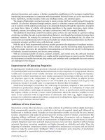
for all w. This, in turn, implies that the associated sensitivity singular values satisfy
(30.156)
for all w, where
(30.157)
• From the above sensitivity singular value relationship, we obtain the follow celebrated KBF loop
margins:
infinite upward gain margin,
at least (6 dB) downward gain margin,
at least ±60° phase margin.
The above gain margins apply to simultaneous and independent gain perturbations when the
loop is broken at the output. The same holds for the above phase margins. The above margins
are NOT guaranteed for simultaneous gain and phase perturbations. It should be noted that
these margins can be easily motivated using elementary SISO Nyquist stability arguments [2,8].
• From the above sensitivity singular value relations, we obtain the following complementary
sensitivity singular value relationship:
(30.158)
for all w, where
(30.159)
2. Recovery of Target Loop L
o
Using Model-Based Compensator. The second step is to use a model-
based compensator K
opt
= [ A − BG
c
− H
f
C, H
f
, G
c

] where G
c
is found by solving the CARE
with A, B, M = C, R = with
ρ
a small positive scalar. Since r is small, we call this a
cheap control problem.
• If the plant P = [A, B, C] is minimum phase, then it can be shown that
(30.160)
(30.161)
for some orthonormal W (i.e., W
T
W = WW
T
= I )
(30.162)
In such a case, PK
opt
≈ L
o
for small
ρ
and hence PK
opt
will possess stability margins that are
close to those of L
o
(at the plant output)—whatever method was used to design L
o
. It must

be noted that the minimum phase condition on the plant P is a suficient condition. It is
not necessary. Moreover, G
c
need not be computed using a CARE. In fact, any G
c
which (1)
satisfies a limiting condition for some invertible matrix W and which (2)
ensures that A − BG
c
is stable (for small r), will result in LTR at the plant output. This result
s
max
S
KF
jw()[]
1
s
min
S
KF
jw()[]
−1

1 0dB()≤=
S
KF
jw() IG
KF
jw()+[]
−1

=
1
2

s
max
T
KF
jw()[]s
max
IS
KF
jw()–[]= 1 s
max
S
KF
jw()[]26dB()≤+≤
T
KF
IS
KF
G
KF
=–= 1 G
KF
+[]
−1
rI
n
u

n
u
×
X
r 0
+
→
lim 0=
rG
c
r 0
+
→
lim WC=
PK
opt
r 0
+
→
lim L
o
=
rG
c
r
0
+
→
lim WC=
0066_Frame_C30 Page 28 Thursday, January 10, 2002 4:44 PM

©2002 CRC Press LLC


31

Adaptive and Nonlinear

Control Design

31.1 Introduction

31.2 Lyapunov Theory for Time-Invariant Systems

31.3 Lyapunov Theory for Time-Varying Systems

31.4 Adaptive Control Theory

Regulation and Tracking Problems • Certainty Equivalence
Principle • Direct and Indirect Adaptive Control • Model
Reference Adaptive Control (MRAC) • Self-Tuning
Controller (STC)

31.5 Nonlinear Adaptive Control Systems

31.6 Spacecraft Adaptive Attitude Regulation Example

31.7 Output Feedback Adaptive Control

31.8 Adaptive Observers and Output Feedback Control


31.9 Concluding Remarks

31.1 Introduction

The most important challenge for modern control theory is that it should deliver acceptable performance
while dealing with poor models, high nonlinearities, and low-cost sensors under a large number of op-
erating conditions. The difficulties encountered are not peculiar to any single class of systems and they
appear in virtually every industrial application. Invariably, these systems contain such a large amount of
model and parameter uncertainty that “fixed”controllers can no longer meet the stability and performance
requirements. Any reasonable solution for such problems must be a suitable amalgamation between
nonlinear control theory, adaptive elements, and information processing. Such are the factors behind
the birth and evolution of the field of adaptive control theory, strongly motivated by several practical
applications such as chemical process control and design of autopilots for high-performance aircraft,
which operate with proven stability over a wide variety of speeds and altitudes.
A commonly accepted definition for an adaptive system is that it is any physical system that is designed
from an adaptive standpoint!

1

All existing stability and convergence results, in the field of adaptive control
theory, hinge on the crucial assumption that the unknown parameters must occur linearly within the
plant containing known nonlinearities. Conceptually, the overall process makes the parameter estimates
themselves as state variables, thus enlarging the dimension of the state space for the original system. By
nature, adaptive control solutions for both linear and nonlinear dynamical systems lead to nonlinear
time-varying formulations wherein the estimates of the unknown parameters are updated using
input–output data. A parameter adaptation mechanism (typically nonlinear) is used to update the param-
eters within the control law. Given the nonlinearity due to adaptive feedback, there is the need to ensure
that the closed-loop stability is preserved. It is thus an unmistakable fact that the fields of adaptive control
and nonlinear system stability are intrinsically related to one another and any new insights gained in one


Maruthi R. Akella

The University of Texas at Austin
©2002 CRC Press LLC


32

Neural Networks

and Fuzzy Systems

32.1 Neural Networks and Fuzzy Systems

32.2 Neuron Cell

32.3 Feedforward Neural Networks

32.4 Learning Algorithms for Neural Networks

Hebbian Learning Rule • Correlation Learning
Rule • Instar Learning Rule • Winner Takes All
(WTA) • Outstar Learning Rule • Widrow–Hoff LMS
Learning Rule • Linear Regression • Delta Learning
Rule • Error Backpropagation Learning

32.5 Special Feedforward Networks

Functional Link Network • Feedforward Version of the
Counterpropagation Network • WTA

Architecture • Cascade Correlation Architecture • Radial
Basis Function Networks

32.6 Recurrent Neural Networks

Hopfield Network • Autoassociative
Memory • Bidirectional Associative Memories (BAM)

32.7 Fuzzy Systems

Fuzzification • Rule Evaluation • Defuzzification • Design
Example

32.8 Genetic Algorithms

Coding and Initialization • Selection and Reproduction •
Reproduction • Mutation

32.1 Neural Networks and Fuzzy Systems

New and better electronic devices have inspired researchers to build intelligent machines operating in a
fashion similar to the human nervous system. Fascination with this goal started when McCulloch and
Pitts (1943) developed their model of an elementary computing neuron and when Hebb (1949) intro-
duced his

learning rules

. A decade later Rosenblatt (1958) introduced the

perceptron


concept. In the early
1960s Widrow and Holf (1960, 1962) developed intelligent systems such as ADALINE and MADALINE.
Nillson (1965) in his book

Learning Machines

summarized many developments of that time. The pub-
lication of the Mynsky and Paper (1969) book, with some discouraging results, stopped for some time the
fascination with artificial neural networks, and achievements in the mathematical foundation of the

back-
propagation

algorithm by Werbos (1974) went unnoticed. The current rapid growth in the area of neural
networks started with the Hopfield (1982, 1984) recurrent network, Kohonen (1982) unsupervised training
algorithms, and a description of the backpropagation algorithm by Rumelhart et al. (1986).

Bogdan M. Wilamowski

University of Wyoming
©2002 CRC Press LLC


33

Advanced Control of an

Electrohydraulic Axis


33.1 Introduction

33.2 Generalities Concerning ROBI_3, a Cartesian
Robot with Three Electrohydraulic Axes

33.3 Mathematical Model and Simulation of
Electrohydraulic Axes

The Extended Mathematical Model • Nonlinear
Mathematical Model of the Servovalve • Nonlinear
Mathematical Model of Linear Hydraulic Motor

33.4 Conventional Controllers Used to
Control the Electrohydraulic Axis

PID, PI, PD with Filtering

•

Observer

•

Simulation Results
of Electrohydraulic Axis with Conventional Controllers

33.5 Control of Electrohydraulic Axis with
Fuzzy Controllers

33.6 Neural Techniques Used to Control the

Electrohydraulic Axis

Neural Control Techniques

33.7 Neuro-Fuzzy Techniques Used to Control the
Electrohydraulic Axis

C ontrol Structure

33.8 Software Considerations

33.9 Conclusions

33.1 Introduction

Due to the development of technology in the last few years, robots are seen as advanced mechatronic
systems which require knowledge from mechanics, actuators, and control in order to perform very
complex tasks. Different kinds of servo-systems, especially electrohydraulic, could be met at the executive
level of the robots. Taking into account the most advanced control approaches, this paper deals with the
implementation of advanced controllers besides conventional ones which are used in an electrohydraulic
system. The considered electrohydraulic system is one of the axes of a robot. These robots possess three
or more electrohydraulic axes, which are identical with the axis studied in this chapter.
An electrohydraulic axis whose mathematical model (MM) is described in this chapter presents a
multitude of nonlinearities. Conventional controllers are becoming increasingly inappropriate to control
the systems with an imprecise model where many nonlinearities are manifested. Therefore, advanced
techniques such as neural networks and fuzzy algorithms are deeply involved in the control of such
systems. Neural networks, initially proposed by McCulloch and Pitts, Rosenblatt, Widrow, had several

Florin Ionescu


University of Applied Sciences

Crina Vlad

Politeknica University of Bucharest

Dragos Arotaritei

Aalborg University Esbjerg
©2002 CRC Press LLC