Bishop, Robert H. - The Mechatronics Handbook [CRC Press 2002] Part 13 pot
Bạn đang xem bản rút gọn của tài liệu. Xem và tải ngay bản đầy đủ của tài liệu tại đây (198.96 KB, 5 trang )
We will see that for a closed-loop system, the polar plot of the loop transfer function is useful in
determining the stability of the system. The polar plots of some simple systems are shown in Fig. 27.9.
27.4 Log-Magnitude Versus Phase Plots
Another approach to presenting the frequency response of a system by a single graph is to plot its
logarithmic magnitude versus the phase angle over a frequency range of interest. The resulting curve is
a function of the frequency
ω
. Such log-magnitude versus phase plots are called Nichols charts.
Advantages of the Nichols chart are that the relative stability of the closed-loop system can be deter-
mined quickly and that the process of closed-loop compensation can be carried out easily. The Nichols
charts of the systems in Fig. 27.9 are depicted in Fig. 27.10 for comparison. Figure 27.11 displays three
different frequency-response curves of the second-order system
FIGURE 27.7 Polar plots of system with various system types as
ω
→ 0.
FIGURE 27.8 Polar plots of system with various relative degrees as
ω
→ ∞.
Gs()
ω
n
2
s
2
2Vw
n
s
ω
n
2
++
=
0066_frame_C27 Page 8 Wednesday, January 9, 2002 7:10 PM
©2002 CRC Press LLC
28
Kalman Filters
as Dynamic System
State Observers
28.1 The Discrete-Time Linear Kalman Filter
Linearization of Dynamic and Measurement System
Models • Linear Kalman Filter Error Covariance
Propagation • Linear Kalman Filter Update
28.2 Other Kalman Filter Formulations
The Continuous–Discrete Linear Kalman Filter
• The Continuous–Discrete Extended Kalman Filter
28.3 Formulation Summary and Review
28.4 Implementation Considerations
28.1 The Discrete-Time Linear Kalman Filter
Distilled to its most fundamental elements, the Kalman filter [1] is a predictor-corrector estimation
algorithm that uses a dynamic system model to predict state values and a measurement model to correct
this prediction. However, the Kalman filter is capable of a great deal more than just state observation in
such a manner. By making certain stochastic assumptions, the Kalman filter carries along an internal metric
of the statistical confidence of the estimate of individual state elements in the form of a covariance matrix.
The essential properties of the Kalman filter are derived from the requirements that the state estimate be
• a linear combination of the previous state estimate and current measurement information
• unbiased with respect to the true state
• and optimal in terms of having minimum variance with respect to the true state.
Starting with these basic requirements an elegant and efficient formulation for the implementation of
the Kalman filter may be derived.
The Kalman filter processes a time series of measurements to update the estimate of the system state
and utilizes a dynamic model to propagate the state estimate between measurements. The observed
measurement is assumed to be a function of the system state and can be represented via
(28.1)
where
Y
(
t
) is an
m
dimensional observable,
h
is the nonlinear measurement model,
X
(
t
) is the
n
dimensional system state,
ββ
ββ
is a vector of modeling parameters, and
v
(
t
) is a random process accounting
for measurement noise.
Y t() h X t(),
ββ
ββ
,t()v t()+=
Timothy P. Crain II
NASA Johnson Space Center
0066_Frame_C28 Page 1 Wednesday, January 9, 2002 7:19 PM
©2002 CRC Press LLC
29
Digital Signal Processing
for Mechatronic
Applications
29.1 Introduction
29.2 Signal Processing Fundamentals
Continuous-Time Signals • Discrete-Time Signals
29.3 Continuous-Time to Discrete-Time Mappings
Discretization •
s
-Plane to
z
-Plane Mappings
• Frequency Domain Mappings
29.4 Digital Filter Design
IIR Filter Design • FIR Filter Design • Computer-Aided
Design of Digital Filters • Filtering Examples
29.5 Digital Control Design
Digital Control Example
29.1 Introduction
Most engineers work in the world of mechatronics as there are relatively few systems that are purely
mechanical or electronic. There are a variety of means by which electrical systems augment mechanical
systems and vise versa. For example, most microprocessors found in a computer today have some sort
of heat sink and perhaps a fan attached to them to keep them within their operational temperature zone.
Electrical systems are widely employed to monitor and control a wide variety of mechanical systems.
With the advent of inexpensive digital processing chips, digital filtering and digital control for mechanical
systems is becoming commonplace. Examples of this can be seen in every automobile and most household
appliances. For example, sensor signals used in monitoring and controlling of mechanical systems require
some form of signal processing. This signal processing can range from simply “cleaning-up” the signal
using a low pass filter to more advanced analyses such as torque and power monitoring in a DC servo
motor. This chapter presents a brief overview of digital signal processing methods suitable for mechanical
systems. Since this chapter is limited in space, it does not give any derivation or details of analysis. For
a more detailed discussion, see references [1,2].
29.2 Signal Processing Fundamentals
A few fundamental concepts on signal processing must be introduced before a discussion of filtering or
control can be undertaken.
Bonnie S. Heck
Georgia Institute of Technology
Thomas R. Kurfess
Georgia Institute of Technology
©2002 CRC Press LLC
30
Control System Design
Via
H
2
Optimization
30.1 Introduction
30.2 General Control System Design Framework
Central Idea: Design Via Optimization • The
Signals • General
H
2
Optimization Problem • Generalized
Plant • Closed Loop Transfer Function
Matrices • Overview of
H
2
Optimization Problems to Be
Considered
30.3
H
2
Output Feedback Problem
Hamiltonian Matrices
30.4
H
2
State Feedback Problem
Generalized Plant Structure for State Feedback • State
Feedback Assumptions
30.5
H
2
Output Injection Problem
Generalized Plant Structure for Output Injection •
Output Injection Assumptions
30.6 Summary
30.1 Introduction
This chapter addresses control system design via
H
2
(quadratic) optimization. A unifying framework
based on the concept of a generalized plant and weighted optimization permits designers to address state
feedback, state estimation, dynamic output feedback, and more general structures in a similar fashion.
The framework permits one to easily incorporate design parameters and/or weighting functions that may
be used to influence the outcome of the optimization, satisfy desired design specifications, and systematize
the design process. Optimal solutions are obtained via well-known Riccati equations; e.g., Control
Algebraic Riccati Equation (CARE) and Filter Algebraic Riccati Equation (FARE). While dynamic weight-
ing functions increase the dimension of the Riccati equations being solved, solutions are readily obtained
using today’s computer-aided design software (e.g., MATLAB, robust control toolbox,
µ
-synthesis tool-
box, etc.).
In short,
H
2
optimization generalizes all of the well-known quadratic control and filter design
methodologies:
• Linear Quadratic Regulator (LQR) design methodology [7,11],
• Kalman–Bucy Filter (KBF) design methodology [5,6],
• Linear Quadratic Gaussian (LQG) design methodology [4,10,11].
H
2
optimization may be used to systematically design constant gain state feedback control laws, state
estimators, dynamic output controllers, and much more.
Armando A. Rodriguez
Arizona State University
0066_Frame_C30 Page 1 Thursday, January 10, 2002 4:43 PM
©2002 CRC Press LLC