Bishop, Robert H. - The Mechatronics Handbook [CRC Press 2002] Part 11 ppt
Bạn đang xem bản rút gọn của tài liệu. Xem và tải ngay bản đầy đủ của tài liệu tại đây (174.58 KB, 4 trang )
the amplitude spectral density gives a continuous display of the amplitude density spectrum, which in
this case is in the form of impulses, rather than just a number.
Similarly the Fourier transform of a train of impulses of the form
(23.27)
is given by
(23.28)
Energy and Power Spectral Density
6
Suppose x(t) is an aperiodic signal with a Fourier transform X( f ), then its energy is given by
(23.29)
This is Parseval’s theorem and it shows that the principle of conservation of energy in the time and
frequency domains holds. The amplitude spectrum X( f) can be expressed as
TABLE 23.5 Properties of the Fourier Transform
Property Signal Description Fourier Transform
Linearity ax + by ; a, b constants aX + bY
Evenness and oddness
Time shift e
−j2
π
f
τ
X
Time scale
x
Time reversal
x(−t) X
∗
Duality
Xx
Time convolution
x ∗ yXY
Frequency convolution
xy X ∗ Y
Modulation X
Time differentiation
Frequency differentiation t
n
x
Integration
Correlation YX
Parseval’s theorem
t() t() f()
f()
xt–() xt()=
xt–() x– t()=
Xf() 2 xt() 2
π
ft()cos td
0
∞
∫
=
Xf() 2– xt() 2
π
ft()sin td
0
∞
∫
=
xt t–() f()
at()
1
a
X
f
a
f()
t() f–()
t() t() f() f()
t() t() f()
f()
xt()e
j2
π
f
0
t
ff
0
–()
d
n
dt
n
xt() j2pf()
n
Xf()
t()
j
2p
n
d
n
df
n
Xf()
x
τ
()
τ
d
∞–
∞
∫
1
j2
π
f
Xf()
1
2
X 0()
δ
f()+
R
xy
τ
() yt()xt
τ
–()td
∞–
∞
∫
= f–()
f()
xt()
2
td
∞–
∞
∫
Xf()
2
fd
∞–
∞
∫
pt()
δ
tnT–()
n=∞–
∞
∑
=
Pf()
1
T
δ
fkF
s
–(), F
s
k=∞–
∞
∑
1
T
==
ER
xx
0() xt()
2
td
∞–
∞
∫
Xf()
2
fd
∞–
∞
∫
== =
Xf() Xf() Xf()∠=
0066_Frame_C23 Page 15 Wednesday, January 9, 2002 1:53 PM
©2002 CRC Press LLC
the amplitude spectral density gives a continuous display of the amplitude density spectrum, which in
this case is in the form of impulses, rather than just a number.
Similarly the Fourier transform of a train of impulses of the form
(23.27)
is given by
(23.28)
Energy and Power Spectral Density
6
Suppose x(t) is an aperiodic signal with a Fourier transform X( f ), then its energy is given by
(23.29)
This is Parseval’s theorem and it shows that the principle of conservation of energy in the time and
frequency domains holds. The amplitude spectrum X( f ) can be expressed as
TABLE 23.5 Properties of the Fourier Transform
Property Signal Description Fourier Transform
Linearity ax + by ; a, b constants aX + bY
Evenness and oddness
Time shift e
−j2
π
f
τ
X
Time scale
x
Time reversal
x(−t) X
∗
Duality
Xx
Time convolution
x ∗ yXY
Frequency convolution
xy X ∗ Y
Modulation X
Time differentiation
Frequency differentiation t
n
x
Integration
Correlation YX
Parseval’s theorem
t() t() f()
f()
xt–() xt()=
xt–() x– t()=
Xf() 2 xt() 2
π
ft()cos td
0
∞
∫
=
Xf() 2– xt() 2
π
ft()sin td
0
∞
∫
=
xt t–() f()
at()
1
a
X
f
a
f()
t() f–()
t() t() f() f()
t() t() f()
f()
xt()e
j2
π
f
0
t
ff
0
–()
d
n
dt
n
xt() j2pf()
n
Xf()
t()
j
2p
n
d
n
df
n
Xf()
x
τ
()
τ
d
∞–
∞
∫
1
j2
π
f
Xf()
1
2
X 0()
δ
f()+
R
xy
τ
() yt()xt
τ
–()td
∞–
∞
∫
= f–()
f()
xt()
2
td
∞–
∞
∫
Xf()
2
fd
∞–
∞
∫
pt()
δ
tnT–()
n=∞–
∞
∑
=
Pf()
1
T
δ
fkF
s
–(), F
s
k=∞–
∞
∑
1
T
==
ER
xx
0() xt()
2
td
∞–
∞
∫
Xf()
2
fd
∞–
∞
∫
== =
Xf() Xf() Xf()∠=
0066_Frame_C23 Page 15 Wednesday, January 9, 2002 1:53 PM
©2002 CRC Press LLC
The Discrete Fourier Transform
Consider a finite length sequence that is zero outside the interval 0
≤
k
≤
N
−
1. Evaluation of
the
z
transform
X
(
z
) at
N
equally spaced points on the unit circle
z
=
exp(
i
ω
k
T
)
=
exp[
i
(2
π
/
NT
)
kT
] for
k
=
0, 1,…,
N
−
1 defines the
discrete Fourier transform
(DFT) of a signal
x
with a sampling period
h
and
N
measurements:
(23.60)
Notice that the discrete Fourier transform is only defined at the discrete frequency points
(23.61)
In fact, the discrete Fourier transform adapts the Fourier transform and the
z
transform to the practical
requirements of finite measurements. Similar properties hold for the discrete Laplace transform with
z
=
exp(
sT
), where
s
is the Laplace transform variable.
The Transfer Function
Consider the following discrete-time linear system with input sequence {
u
k
} (stimulus) and output sequence
{
y
k
} (response). The dependency of the output of a linear system is characterized by the convolution-
type equation and its
z
transform,
(23.62)
where the sequence {
v
k
} represents some external input of errors and disturbances and with
Y
(
z
)
=
ᐆ
{
y
},
U
(
z
)
=
ᐆ
{
u
},
V
(
z
)
=
ᐆ
{
v
} as output and inputs. The
weighting function h
(
kT
)
=
, which is zero
for negative
k
and for reasons of causality is sometimes called
pulse response
of the digital system (compare
impulse response
of continuous-time systems). The pulse response and its
z
transform, the
pulse transfer
function
,
(23.63)
determine the system’s response to an input
U
(
z
); see Fig. 23.18. The pulse transfer function
H
(
z
) is obtained
as the ratio
(23.64)
FIGURE 23.18
Block diagram with an assumed transfer function relationship
H
(
z
) between input
U
(
z
), disturbance
V
(
z
), intermediate
X
(
z
), and output
Y
(
z
).
{x
k
}
k=0
N−1
X
k
DFT xkT(){} x
l
iw
k
lT–()exp
l=0
N−1
∑
Xe
iw
k
T
()== =
{X
k
}
k=0
N−1
w
k
2p
NT
k, for k 0, 1,…, N 1–==
y
k
h
m
u
k−m
v
k
+
m=0
∞
∑
h
k−m
u
m
v
k
, k+
m=−∞
k
∑
…, −1, 0, 1, 2,…== =
Yz() Hz()Uz() Vz()+=
{h
k
}
k=0
∞
Hz() ᐆ hkT(){}h
k
z
k–
k=0
∞
∑
==
Hz()
Xz()
Uz()
=
U(z) X(z) Y(z)
V(z)
Σ
H(z)
0066_Frame_C23 Page 33 Wednesday, January 9, 2002 1:55 PM
©2002 CRC Press LLC
24
State Space Analysis
and System Properties
24.1 Models: Fundamental Concepts
24.2 State Variables: Basic Concepts
Introduction • Basic State Space Models • Signals and State
Space Description
24.3 State Space Description for Continuous-Time
Systems
Linearization • Linear State Space models • State Similarity
Transformation • State Space and Transfer Functions
24.4 State Space Description for Discrete-Time
and Sampled Data Systems
Linearization of Discrete-Time Systems • Sampled Data
Systems • Linear State Space Models • State Similarity
Transformation • State Space and Transfer Functions
24.5 State Space Models for Interconnected
Systems
24.6 System Properties
Controllability, Reachability, and Stabilizability
• Observability, Reconstructibility, and Detectability
• Canonical Decomposition • PBH Test
24.7 State Observers
Basic Concepts • Observer Dynamics • Observers and
Measurement Noise
24.8 State Feedback
Basic Concepts • Feedback Dynamics • Optimal State
Feedback. The Optimal Regulator
24.9 Observed State Feedback
Separation Strategy • Transfer Function Interpretation for
the Single-Input Single-Output Case
24.1 Models: Fundamental Concepts
An essential connection between an engineer/scientist and a system relies on his/her ability to describe
the system in a way which is useful to understand and to quantify its behavior.
Any description supporting that connection is a
model
. In system theory, models play a fundamental
role, since they are needed to analyze, to synthesize, and to design systems of all imaginable sorts.
There is not a unique model for a given system. Firstly, the need for a model may obey different
purposes. For instance, when dealing with an electric motor, we might be interested in the electro-
mechanical energy conversion process, alternatively, we might be interested in modelling the motor either
as a thermal system, or as a mechanical system to study vibrations, the strength of the materials, and so on.
Mario E. Salgado
Universidad Técnica Federico
Santa María
Juan I. Yuz
Universidad Técnica Federico
Santa María
©2002 CRC Press LLC