4
3
STRESS STATE VARIABLES
where
u,
=
pore-air pressure
x
=
a parameter related to the degree
of
saturation
of
The magnitude of
the
x
parameter is unity for a saturated
soil and zero for a dry soil. The relationship between
x
and
the degree of saturation,
S,
was obtained experimentally.
Experiments were performed on cohesionless silt (Donald,
1961)
and compacted soils (Blight
l%l),
as shown in Fig.
3.l(a)
and
3.

I@),
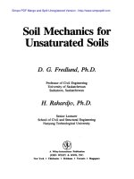
respectively. Figure
3.1
demonstrates
the influence of the soil type on the
x
parameter (Bishop
and Henkel,
1962).
Bishop et al.
(1960)
presented the re-
sults of triaxial tests performed on saturated and unsatu-
rated soils in an attempt to substantiate the use of Bishop’s
equation [i.e., Eq.
(3.3)].
Bishop and Donald
(1961)
published the results of triax-
ial tests on an unsaturated silt in which the total, pore-air,
and pore-water pressures were controlled independently.
During the tests, the confining, pore-air, and pore-water
the soil.
1
.o
0.8
0.6
X
0.4
0.2

Degree
of
saturation,
S
(%)
(a)
1
.o
0.8
0.6
X
0.4
2
-Boulder clay
3
-
Boulder
clay
4-Clay -shale
‘0
20
40
60
00
100
Degree of saturation,
S
(%)
(b)
Figure

3.1
The relationship between the
x
parameter and the
degree
of
saturation,
S.
(a)
x
values
for
a cohesionless
silt
(after
Donald,
1961);
(b)
x
values
for
compacted
soils
(after
Blight,
1961).
pressures (Le.,
a,,
u,,
and

u,)
were varied in such a way
that the
(u3
-
u,)
and
(u,
-
uw)
variables remained con-
stant. The results showed that the stress-strain curve
re-
mained monotonic during these changes. This lent credi-
bility to the use of
Eq.
(3.3);
however, the test results
equally justify the use of independent stress state variables.
Aitchison
(1961)
proposed the following effective stress
equation at the Conference
on
Pore Pressure and Suction
in Soils, London, in
1960:
uf
=
u

+
J.p”
(3.4)
where
p”
=
pore-water pressure deficiency
J.
=
a parameter with values ranging fmm zero to one.
Jennings
(1961)
also proposed an effective stress equa-
tion at the same conference:
0)
=
(I
+
pp”
(3.5)
where
p”
=
negative pore-water pressure taken as a positive
value
6
=
a statistical factor
of
the same type as the contact

area. This factor should
be
measured experimen-
Equations
(3.2), (3.3), (3.4),
and
(3.5)
are equivalent
when the pore-air pressure used in all four equations
is
the
same (i.e.,
0‘
=
x
=
1c,
=
6).
Only Bishop’s form
[i.e.,
Eq.
(3.3)]
references the total and pore-water pressures to
the pore-air pressure. The other equations simply use gauge
pressures which are referenced to the external air pressure.
Jennings and Burland
(1962)
appear to
be

the first to sug-
gest that Bishop’s equation did not provide an adequate
relationship between volume change and effective stress for
most soils, particularly those below a critical degree
of
sat-
uration. The critical degree of saturation was estimated to
be
approximately
20%
for silts and sands, and as high
as
8540%
for clays.
Coleman
(1962)
suggested
the
use
of “reduced” stress
variables,
(a,
-
u,),
(u3
-
u,),
and
(u,
-

u,),
to represent
the axial, confining, and pore-water pressures, respec-
tively, in triaxial tests. The constitutive relations for vol-
ume change in unsaturated soils were then formulated in
terms of the above stress variables.
In
1963,
Bishop and Blight reevaluated the proposed ef-
fective stress equation [Le.,
E!q.
(3.3)]
for unsaturated soils.
It was noted that a variation in matric suction,
(u,
-
uw),
did not result in the same change in effective stress as did
a change in the net normal stress,
(a
-
u,).
A graphical
presentation was suggested for volume change
(or
void ra-
tio change,
Ae)
versus the
(a

-
u,)
and
(u,
-
u,)
stress
variables. This further reinforced the use
of
the stress state
variables in
an
independent
manner.
Blight
(1965)
con-
cluded that the proposed effective stress equation depends
tally.

3.1
HISTORY
OF
THE
DESCRIPTION
OF
THE STRESS STATE
41
stress variable. Experiments have demonstrated that the ef-
fective stress equation is not single-valued.

Rather,
there
is a dependence on the stress path followed. The
soil
pa-
meter used in the effective
stress
equation appears
t~
be
difficult to evaluate.
In
general, the proposed effective
stress
equations have not received much recent attention in de-
scribing the mechanical behavior of unsaturated soils. In
refemng to the application of Bishop’s effective stress
equation, Morgenstern (1979) stated that the equation has
“-proved to have little impact on practice.
The
parameter
x
when determined
for
volume change behaviour was found
to differ
when
determined for shear strength.”
Probably more impottant
than

the above experimental dif-
ficulties is the philosophical difficulty in justifying the use
of soil properties in the description
of
a stress state.
Mor-
genstern (1979) stated,
“The
effective stress is a
stress
variable and hence related to equilibrium considerations
alone while [Equation 3.31 contains a parameter,
x,
that
bears
on constitutive behavior. This parameter is found
by assuming that the behavior of a soil
can
be
expressed
uniquely in
terms
of a single effective stress variable and
by matching unsaturated behaviour with saturated behav-
ior in order to calculate
x.
Normally, we link equilibrium
considerations to deformations through constitutive behav-
ior and
do

not introduce constitutive behavior directly
into the stress variable.” Reexamination of
the
proposed
effective stress equations
has
led many researchers to sug-
gest the
use
of independent stress state variables [e.g.,
(a
-
u,)
and
(u,
-
u,)]
to
describe the mechanical behav-
ior of unsaturated soils.
Fredlund and Morgenstern (1977) presented a theoretical
stress analysis of an unsaturated soil on the basis of multi-
phase continuum mechanics. The unsaturated soil was con-
sidered
as
a four-phase system.
The
soil particles were as-
sumed to be incompressible and the soil was treated as
though it were chemically inert. These assumptions

are
consistent with those used in saturated soil mechanics.
The analysis concluded that any two of three possible
normal stress variables can be used
to
describe the stress
state of
an
unsaturated soil.
In
other words, there
are
three
possible combinations which can be used
as
stress
state
variables for an unsaturated soil. These are: 1)
(a
-
u,)
and
(u,
-
u,),
2)
(a
-
u,)
and

(u,
-
u,),
and 3)
(a
-
u,)
and
(a
-
u,).
In
a three-dimensional stress analysis, the
stress state variables
of
an
unsaturated soil form
two
in-
dependent stress tensors. These are discussed in the follow-
ing sections. The proposed
stress
state variables for unsat-
urated soils have
also
been experimentally tested (Fredlund,
1973).
The stress state variables can then be used to formulate
constitutive equations to describe the shear strength behav-
ior and the volume change behavior of Unsaturated soils.

This eliminates the need
to
find a single-valued effective
stress equation that is applicable to
both
shear strength and
volume change problems. The use of independent
stress
on the type of process to which the soil was subjected.
Burland (1954, 1965) fulther questioned the validity of the
proposed effective stress equation, and suggested that the
mechanical behavior of unsaturated soils should be inde-
pendently related to the
stress
variables,
(a
-
u,)
and
(u,
-
u,),
whenever possible.
Richards
(1966)
incorporated a solute suction component
into the effective stress equation:
(3.6)
Q’
=

(I
-
U,
+
xm(h,
+
u,)
+
xS(h,
+
u,)
where
xm
=
effective stress parameter for matric suctian
h,
=
matric suction
=
effective
stress
pameter for solute suction
h,
=
solute suction.
Little reference has subsequently been made to this equa-
tion. Aitchison (1967) pointed out the complexity associ-
ated
with
the

x
parameter. He stated that a specific value
of
x
may only relate to a single combination of
(a)
and
(u,
-
ro,)
for a particular stress path. It was suggested that
the terms
(a)
and
(u,
-
u,)
be separated in analyzing the
behavior of unsaturated soils. Later, constitutive relation-
ship data (Aitchison and Woodbum, 1969) were presented
in
accordance with the proposed independent stress
vari-
ables.
Matyas and Radhakrishna (1968) introduced the concept
of “state parameters” in describing the volumetric behav-
ior of unsaturated soils. Volume change was presented
as
a three-dimensional surface with respect to the state param-
eters,

(a
-
u,)
and
(u,
-
u,).
Barden et al. (1969a) also
suggested that the volume change of unsaturated soils be
analyzed
in
terms of the separate components of applied
stress,
(a
-
u,),
and suction,
(u,
-
u,).
Brackley (1971) examined the application of the effective
stress principle to the volume change behavior of unsatu-
rated soils. He concluded from his test results that there
was
a limit to the use of a single-valued effective stress
equation.
Aitchison (1965a, 1973) presented an effective stress
equation slightly modified from that of Richards (1966):
(3.7)
a’

=
a
+
x,p:
+
x,p:
where
p$
=
matric suction,
(u,
-
u,)
p,”
=
solute suction
xm
and
xs
=
soil parameters which are normally
within
the range of 0-1, which are dependent upon
the stress path.
The above history shows that considerable effort has
been
extended
in
the search for a single-valued effective stress
equation for unsaturated soils. Numerous effective stress

equations have been proposed. All equations incorporate
a
soil parameter
in
order
to
form a single-valued effective

42
3
STRESSSTATEVAWLES
state variables has produced a more meaningful description
of unsaturated
soil
behavior, and forms the basis for for-
mulations
in
this book.
3.2
STRESS
STATE
VARIABLES
FOR
UNSA"RATED
SOILS
The mechanical behavior of soils is controlled by the same
stress variables which control the equilibrium of the soil
structure. Therefore, the stress variables required to de-
scribe the equilibrium of the soil structure can be taken as
the stress state variables for the soil. The stress state vari-

ables must be expressed
in
terms of the measurable stresses,
such as the total
stress,
u,
the pore-water pressure,
uwr
and
the pore-air pressure,
u,.
An
equilibrium stress analysis
can be performed for an unsaturated soil after considering
the state of stress at a point
in
the soil.
3.2.1
Equilibrium
Analysis
for
Unsaturated
Soils
There
are
two
types
of forces that can act on
an
element

of
soil. These
are
body forces and surface forces. Body fowes
act through the centroid
of
the soil element, and are ex-
pressed as a force per unit volume. Gravitational and
in-
teraction forces between phases are examples of body
forces. Surface forces, such as external loads, act only on
the
boundary surface
of
the soil element. The average value
of a surface force per unit area tends to a limiting value as
the surface area approaches zero. This limiting value is
called the stress vector or the surface traction on a given
surface. The component of the stress vector perpendicular
to a plane is defined as a normal stress,
u.
The stress com-
ponents parallel to a plane
am
referred to as shear stresses,
an
infinite number of planes (or surfaces) that
can
be
passed through a

point
in a soil mass. The stress
state at a point can be analyzed by considering all
the
stresses acting on the planes that form a cubical element
of
infinitesimal dimensions. In addition, body forces acting
through the centroid of the soil element should be consid-
ered.
A
cubical element that is completely enclosed by
imaginary, unbiased boundaries yields the conventional
free
body used for a stress equilibrium andysis (Fung,
1969;
Biot,
1955;
Hubbert and Rubey,
1959).
Figure
3.2
shows
a
cubical soil element
with
infinitesimal dimensions of
dr,
dy,
and
dz

in
the Cartesian coordinate system. The normal
and shear stresses on each plane of the element
are
illus-
trated in Fig.
3.2.
The
body
forces are not shown.
Nod
and
Shear
Stresses
on
a
Soil
Element
Normal and shear
stresses
act on every plane in the
x-,
y-,
and z-directions. The normal stress,
u,
has one subscript to
denote the plane on which it acts. Soils are most commonly
subjected to compressive normal stresses. In soil mechan-
ics, a positive nonnal stress is used to indicate a compres-
sion

in
the soil. All the normal stresses shown in Fig.
3.2
are positive or compressive. Opposite directions would in-
dicate negative normal stresses or tensions.
The shear stress,
7,
has two subscripts. The first sub-
script denotes the plane
on
which the shear stress acts, and
the second subscript refers to the direction of the shear
stress. As
an
example, the shear stress,
7R,
acts on the
y-plane and in the z-direction. All of the shear stresses
7.
There

3.2
STRESS
STATE
VARIABLES
FOR
UNSATURATED
SOILS
43
shown in Fig.

3.2
have positive signs. Opposite directions
where
would indicate negative shear
stresses.
Equating the summation of moments about the
x-,
y-,
and z-axes to zero results in the following shear stress re-
lationships:
TYz
=
Try.
(3.10)
The stress components can vary from plane to plane
across an element. The spatial variation of a stress com-
ponent can be expressed
as
its
derivative with respect to
space. The stress variations in the
x-,
y-, and z-directions
are
expressed as stress fields (Fig.
3.2).
Equilibrium Equalions
The stress equilibrium conditions for an unsaturated soil
are presented
in

Appendix
B.
A
cubical element of an
un-
saturated soil (Fig.
3.2)
is used
in
the equilibrium analysis.
Newton’s second law is applied to the soil element by sum-
ming the forces in each direction (i.e.,
x-,
y-,
and
z-directions).
An
equilibrium condition for an unsaturated
soil element implies that the four phases (Le.,
air,
water,
contractile skin, and soil particles) of the soil are in equi-
librium. Each phase is assumed to behave
as
an indepen-
dent, linear, continuous, and coincident
stress
field
in
each

direction.
An
independent equilibrium equation can
be
written for each phase and superimposed using the princi-
ple of superposition. However, this may not give rise to
equilibrium equations with stresses that can
be
measured.
For
example, the interpalticle stresses cannot
be
measured
directly. Therefore, it is necessary to combine the indepen-
dent phases in such a way that measurable stresses appear
in
the equilibrium equation for the soil structure (Le., the
arrangement of soil particles).
The force equilibrium equations
for
the air phase, the
water phase, and contractile skin, together with
the
total
equilibrium equation for the soil element
are
used
in
for-
mulating the equilibrium equation for the soil structure. In

the y-direction, the equilibrium equation
for
the soil struc-
ture has the following form:
374
aua
at
aY
+
-
+
(n,
+
n,)
-
af
*
aY
+
n,(u,
-
uw)-
=
0
(3.11)
rXy
=
shear stress
on
the x-plane in the

uy
=
total normal stress in the ydirection
(or
u,
=
pore-air pressure
f
*
=
interaction function between the equi-
librium
of
the soil structure and the
equilibrium of the contractile skin
(ay
-
u,)
=
net normal stress in the ydirection
n,
=
porosity relative
to
the water phase
n,
=
porosity relative to the contractile skin
u,
=

pore-water pressure
r4
=
shear stress on the z-plane
in
the
n,
=
porosity relative
to
the soil particles
g
=
gravitational acceleration
p,
=
soil particle density
ydirection
on the y-plane)
(u,
-
u,)
=
matric suction
ydirection
F&
=
interaction fom (i.e., body force) be-
tween the water phase and the soil par-
ticles in the y-direction

Fg
=
interaction force (Le., body force) be-
tween
the
air
phase and the soil particles
in
the ydirection.
Similar equilibrium equations can be written for the
x-
and z-directions. The stress variables that control the equi-
librium of the soil structure [i.e.,
Eq.
(3.11)]
also control
the equilibrium of the contractile skin through the interac-
tion function,
f
*.
3.2.2
Stress
State
Variables
Three independent
sets
of normal
stresses
(Le., surface
tractions) can

be
extracted from the equilibrium equation
for the soil structure
[Eq.
(3.11)].
These
are
(by
-
uJ,
(u,
-
u,),
and
(u,),
which govern the equilibrium of the
soil structure and the contractile skin. The components
of
these variables are physically measurable quantities. The
stress variable,
u,,
can
be
eliminated when the soil parti-
cles and the water are assumed to be incompressible. The
((I
-
u,)
and
(u,

-
u,)
are
referred to
as
the
stress
state
variables for
an
unsaturated soil. More specifically, these
are the surface tractions controlling the equilibrium of the
soil structure and the contractile skin.
Similar stress state variables can also be extracted
from
the soil structure equilibrium equations for the
x-
and
zdirections. The complete form of the stress state
for
an
unsaturated soil can therefore
be
written
as
two indepen-
dent stress tensors:
rxy
(@y
-

u,)
74
(3.12)
7yz
(UZ
-
u3
I

44
3
STRESS
STATE VARIABLES
U.
)
Figure
3.3
The
stress state variables for
an
unsaturated
soil.
and
(Ua
-
uw)
1.
(3.13)
The above tensors cannot be combined into one matrix
since the stress variables have different soil properties (i.e.,

porosities) outside the partial differential terms [see Eq.
(3.1
l)].
The porosity terms
are
soil properties that should
not be included in the description of the stress state of a
soil. Figure 3.3 illustrates the
two
independent tensors act-
ing
at a point in
an
unsaturated soil.
In the case of compressible soil particles or pore fluid,
an
additional stress tensor,
u,,
must
be
used to describe the
['"
iuw)
0
O
(Ua
-
uw)
stress state:
u,

0
0
0 0
ua
0
Ma
01
(3.14)
The pore-air and pore-water pressures are usually ex-
pressed in
terms
of gauge pressure. This is a common prac-
tice
in
engineering. Under certain circumstances, such as
when dealing with the gas law, the absolute air pressure
must be used. Figure 3.4 illustrates the relationship
be-
tween
absolute and gauge pressures.
Other
Combinations
of
Stress
State Variables
The equilibrium equation for the soil structure [i.e.,
Eq.
(3.1
l)]
can be formulated in a slightly different manner by

using the pore-water pressure,
u,,
or the total normal
stress,
u,
as a reference (see Appendix
B).
If the pore-
water pressure,
u,,
is used as a reference, the following
combination of stress state variables,
(a
-
u,),
(u,
-
u,),
and
(uw),
can
be
extracted from the equilibrium equations
for the soil sttucture. The stress variable,
u,,
is only of
relevance for soils with compressible soil particles. If the
total normal stress,
a,
is used as a reference, the following

combination of stress state variables,
(a
-
u,),
(a
-
u,),
and
(a),
can be extracted from the equilibrium equations
for the soil structure. The
stress
variable,
u,
can be ignonxl
when the soil particles are assumed to be incompressible.
In summary, there are three possible combinations of
stress state variables that can be used to describe the
stress
state relevant to the soil structure and contmtile skin
in
an
unsaturated soil. These are tabulated
in
Table 3.1. The three
combinations of
stress
state variables
are
obtained from

equilibrium equations for the soil structure which are de-
rived with respect
to
three different references (i.e.,
u,,
u,,
and
a).
However, the
(a
-
u,)
and
(u,
-
u,)
combination
appears to be the most satisfactory for use
in
engineering
practice (Fredlund, 1979; Fmilund and Rahardjo, 1987).
This combination is advantageous because the effects of a
change in total normal stress can be separated from the ef-
fects caused by a change in the pore-water pressure. In
addition, the pore-air pressure is atmospheric (i.e., zero
gauge pressure) for most practical engineering problems.
Gauge
pressures
_.__L
I

-101.3
kPa
-1
Atmosphere
0
kPa
0
Atmosphere
01
0
,
@
Pressure
01
0 0
0
kPa
101.3
kPa
0
Atmosphere
1
Atmosphere
Absolute pressures
-
t
t
Lower limit for
a
gas

Cavitation will occur in ordinary
water measuring systems (air comes out
of
solution)
Figure
3.4
Relationship between absolute
and
gauge
pressures.

3.2
STRESS STATE
VARIABLES
FOR
UNSATURATED
SOW
45
'
Table
3.1 Possible
Combinations
of
Stress
State Variables
for
an
Unsaturated
Soil
Reference Pressure Stress State Variables

Air,
u,
(u
-
u,)
and
(u,
-
u,)
Water,
u,
(0
-
u3
and
(u,
-
u,)
Total,
a
(a
-
u,)
and
(a
-
u,)
Referencing the stress state to the pore-air pressure would
appear to produce the most reasonable and simple combi-
nation of stress state variables. The

(a
-
u,)
and
(u,
-
u,)
combination
is
used throughout this
book,
and these stress
variables are referred to as the net normal stress and the
matric suction, respectively.
3.2.3
Saturated
Soils
as
a Special
Case
of
Unsaturated
Soils
A
saturated soil can be viewed as a special case of
an
un-
saturated soil. The four phases in an unsaturated soil re-
duce to two phases for a saturated soil (Le., soil particles
and water). The phase equilibrium equations for a saturated

soil can be derived using the same theory used for unsat-
urated soils (Appendix
B).
There is also a smooth transition
between the stress state for a saturated soil and that of an
unsaturated soil.
As
an unsaturated soil approaches saturation, the degree
of
saturation,
S,
approaches
100%.
The pore-water pres-
sure,
u,,
appmaches the pore-air pressure,
u,,
and the
ma-
tric suction term,
(u,
-
u,),
goes towards zero. Only the
first stress tensor is retained for a saturated soil when con-
sidering this special case:
7xy by
-
u3

7vr
Tu,
1.
(3.15)
The second stress tensors [Le., Eq.
(3.13)]
disappears
because the matric suction,
(u,
-
u,),
goes
towards zero.
The pore-air pressure term
in
the
first
stress tensor [Le.,
Eq.
(3.12)]
becomes the pore-water pressure,
u,,
in the
stress tensor for a saturated soil [Le.,
Eq.
(3.15)].
The
stress state variables for saturated soils are shown diagram-
matically
in

Fig.
3.5.
The above rationale demonstrates the
smooth transition in
stress
state description when going
from an unsaturated soil to a saturated soil, and vice versa.
The stress tensor for a saturated soil indicates
that
the
difference between the total stress and the pore-water pres-
sure forms a stress state variable that can be used to de-
scribe the equilibrium. This stress state variable,
(a
-
u,),
is commonly refed to
as
effective stress (Terzaghi,
1936).
The so-called effective stress law is essentially a
stress state variable which is requid to describe the me-
(ax
-
uw)
7yx
[
7xr
7yz
(a,

-
u3
(a,
-
u,)
Figure
3.5
The
stress
state
variables
for
a
saturated soil.
chanical behavior of a saturated soil. For the case of com-
pressible soil particles,
an
additional stress tensor (i.e.
,
u,)
should be
used
toedescribe the complete
stress
state for
a
saturated soil (Skempton,
l%l).
3.2.4
Dry

Soh
Evaporation from a soil or airdrying a soil will bring the
soil to a dry condition.
As
the soil dries, the matric suction
increases. Numerous experiments have
shown
that the
ma-
tric suction tends to a common limiting value in
the
range
of
620-980
MPa
as
the water content appmaches
0%
(Fredlund,
1964).
The relationship between the water con-
tent
and the suction of a soil is commonly referred to
as
the
soil-water characteristic curve. Figure
3.6
presents the
soil-water characteristic curve for Regina clay. The gra-
(3

4
b
0
Matric suction, (u.
-
u,)
(kPa)
Figure
3.6
Soil-water characteristic curve for
Regina
clay
(from
Fredlund,
1964).

46
3
STRESS
STATE
VARIABLES
1.
Dune sand
2.
Loamy sand
3.
Calcareous fine sandy loam
4.
Calcareous loam
5.

Silt loam derived from
loess
6.
Young oligotrophous peat soil
0.6
-
10-1
i
io
102
103
io4
10'
io6
Matric suction,
(u.
-
u,)
(kPa)
Figure
3.7
Soil-water characteristic cuwe
for some
Dutch
soils
(from
Koorevaar
et al.,
1983).
vimetric water content, expressed in terms of

(wG,),
is
plotted against matric suction. The void ratio,
e,
is also
plotted against matric suction. The plot shows a decreasing
void ratio and water content as the matric suction
in-
creases. Further results are shown in Fig. 3.7 where the
volumetric water content,
e,,
is plotted versus matric suc-
tion for various soils. The suction approaches
a
value
of
approximately
980
MPa (Le.,
9.8
X
Id
kPa) at
0%
watu
content, as shown
in
both figures. The above plots illus-
trate the continuous nature
of

the water content versus suc-
tion relationship. In other words, there does not appear to
be
any discontinuity
in
this relationship as the soil desatur-
ates. In addition, the void ratio approaches the void ratio
at
the shrinkage limit of the soil as the water content ap-
proaches
0%,
as shown
in
Fig.
3.8.
Even for
a
sandy soil,
2.4
r
I
I
,
-1
0.8
l b+-
-
UA
't
Figure

3.9
The
stress
state variables
for
a dry
soil.
the soil suction continues to increase with drying to
0%
water content.
The effects of a change in matric suction on the mechan-
ical behavior of a soil may become negligible as the soil
approaches
a
completely dry condition. In other words, a
change in matric suction on a dry soil may not produce any
significant change
in
the volume or shear strength of the
soil. For these dry soils, the net normal stress,
(u
-
u,),
may
become the only stress state variable controlling their
behavior.
The effect
of
a matric suction change on the volume
change

of
Regina clay is demonstrated in Fig.
3.8.
As
the
matric suction
of
the soil is increased, the water content is
reduced and the volume
of
the soil decreases. However,
prior to the soil becoming completely dry, the volume of
the soil remains essentially constant regardless of the
in-
crease in matric suction.
As
a soil becomes extremely dry, a matric suction change
may no longer produce any significant changes
in
mechan-
ical properties. Although matric suction remains a stress
state variable,
it
may not
be
required in describing the
be-
havior of the soil. Only the first stress tensor
with
(a

-
u,)
may
be
required for describing the volume decrease of a
dry
soil (Fig.
3.9):
1
On
the other hand, it
may
be
necessary to consider matric
suction
as
a stress state variable when examining the vol-
ume increase or swelling of a dry soil.
J
20
40
60
80
Water content,
w
(%)
Figure
3.8
Void ratio
versus

water content
for
Regina
clay
(from
Fredlund,
1964).
3.3
LIMITING
STRESS
STATE
CONDITIONS
There is a hierarchy with respect to the magnitude
of
the
individual stress components in an unsaturated soil:
(3.17)
u
>
u,
>
u,.

3.4
EXPERIMENTAL TESTING
OF
THE
STRESS
STATE
VARIABLES

47
The hierarchy
in
Eiq.
(3.17) must be maintained in order
to ensure stable equilibrium conditions. Limiting stress
state conditions occur when one of the stress state variables
becomes zero. For example, if the pore-air pressure,
u,,
is
momentarily increased in excess of the total stress,
u,
an
“explosion” of
the
sample may occur. In other words, once
the
(u
-
u,)
variable goes
to
zero,
a limiting stress state
condition is reached. This limiting stress condition is
uti-
lized
in
the pressure plate test [Fig. 3.10(a)].
Let

us sup-
pose
that
an
external air pressure greater than the pre-
water pressure is applied to an unsaturated soil. The sample
could be visualized as being surrounded with a rubber
membrane which is subjected to a total stress equal to the
external air pressure. The pore-air pressure is also equal to
the external air pressure. In this case, the difference
be-
tween the total stress,
(I,
and the pore-air pressure,
u,,
is
zero and the stress state variable
(u
-
u,)
’vanishes. The
stress state variable,
(u,
-
u,),
can be used to describe the
behavior of the unsaturated soil under this limiting condi-
tion.
Another limiting stress state condition occurs when
ma-

tric suction,
(u,
-
u,),
vanishes. If the pore-water pres-
sure is increased
in
excess of the pore-air pressure, the
degree of saturation of the soil approaches 100%. The
backpressure oedometer test [Fig. 3.10(b)] is
an
example
involving the limiting condition where matric suction van-
ishes.
As
the backpressure is applied to the water phase of
an
initially unsaturated soil, the degw of saturation ap-
proaches
100%.
The pore-water pressure approaches the
pore-air pressure and the matric suction goes to zero. The
behavior of the soil can now be described
in
terms of one
stress state variable [Le.,
(a
-
u,)].
A

smooth transition
from the unsaturated case to the saturated case takes place
under the limiting stress state condition
of
pore-air pres-
sure being equal to pore-water pressure.
A
limiting condition occufs
in
saturated soils when the
stress state variable
(a
-
u,)
(i.e., the effective stress)
reaches zero. At this point, the saturated soil becomes
un-
Total stress
=
500
kPa
(External air pressure)
brane
u.
=
5
u-U.
=
500
-

200
=
300kPa
US-
uW
=
500
-
200
=
300 kPa
u
-u,
500
-
500
=
0
kPa
(a)
stable. The soil is said
to
“‘quick.”
A
further increase
in
the pore-water pressure results in a “boil” being formed.
3.4
EXPERIMENTAL
TESTING

OF
THE
STRESS STATE
VARIABLES
The validity
of
the theoretical
stress
state variables should
be experimentally tested.
A
suggested criterion was pro-
posed
by Fredlund and Morgenstern (1977):
“A
suitable set
of
independent
stress
state
variables are those
that
produce
no
distortion
or
volume change
of
an
element when

the individual components
of
the stress state variables are
mod-
ified but
the
stress state variables themselves are kept constant.
Thus the
stress
state variables
for
each phase should produce
equilibrium in that phase when a stress point in
space
is con-
sidel.ed.
”
The experiments used by Fredlund and Morgenstern
(1977) to test the stress state variables
are
called
“null”
tests. The working principle for the “null” tests is based
upon the above criterion for testing
stress
state variables.
The “null” tests consider the overall and water volume
change (or equilibrium conditions) of an unsaturated soil.
An axis-translation technique (Hilf, 1956)
was

used
in
test-
ing the unsaturated soil. Similar null-type tests related to
the shear strength of
an
unsaturated silt were performed by
Bishop and Donald
(l%l).
3.4.1
The Concept
of
Axis
Translation
Difficulties arise
in
testing unsaturated soils with negative
pore-water pressures approaching -1 am (Le.,
zero
ab-
solute pressure). Water in the measuring system may
start
to cavitate when the water pressure approaches -1 atm
(i.e.,
-
101.3 kPa gauge).
As
cavitation occurs, the mea-
suring system becomes filled with air. Then, water from
the measuring system is forced into the soil.

The axis-translation technique is commonly used
in
the
laboratory testing of unsaturated soils
in
order to prevent
Total stress
=
500
kPa
U.
i:
200
kPa
u.
=
200
kPe
Soil
specimen
u
-
uv
=
500
-
200
=
300
kPa

u uv
=
200
-
200
=
0
kPa
(b)
u
-
U,
=
500
-
200
=
300
kP8
Figure
3.10
Tests
performed
at limiting stress state conditions.
(a)
Pressure plate test; (b) back-
pressure oedometer test.

48
3

STRESSSTATEVARIABLES
having to measure pore-water pressures less than zero ab-
solute. The procedure involves a translation of the refer-
ence or pore-air pressure. The pore-water pressure can then
be
referenced to a positive air pressure (Hilf, 1956). Figure
3.11 presents results
from
null-type, pressure plate tests
which demonstrate the use of the axis-translation technique
in
the measurement of matric suctions. This measuring
technique is described in detail in Chapter
4.
Unsaturated
soil specimens were subjected to various external air pres-
sures. The pore-air pressure,
u,,
becomes equal to the ex-
ternally applied air pressure. As a result, the pore-water
pressure,
u,,
undergoes the same pmssure change as the
change in the applied air pressure. In this way, the matric
suction of the soil remains constant regardless of the trans-
lation of both the pore-air and pore-water pressures.
Therefore, the pore-water pressure can be raised to a
pos-
itive value that can
be

measured without cavitation occur-
ring. The axis-translation technique has
been
successfully
applied by numerous researchers to the volume change and
shear strength testing of unsaturated soils (Bishop and Don-
ald, 1961; Gibbs
and
Coffey, 1969b; Fredlund, 1973;
Ho
and Fredlund, 1982a; Gan et al. 1988).
The use of the axis-translation technique requires the
control of the pore-air pressure and the control or mea-
surement of the pore-water pressure. In a triaxial cell, the
pore-air pressure is usually controlled through a coarse co-
rundum disk placed on top of the soil sample. The pore-
water pressure is controlled through a saturated high air
entry ceramic disk sealed to the pedestal
of
the triaxial cell.
The high air entry disk is a porous, ceramic disk which
allows the passage of water, but prevents the flow of free
air.
Continuity between the water in the soil and the water
in
the ceramic disk is necessary
in
order to correctly estab-
lish the matric suction. The matric suction
in

the soil spec-
imen must not exceed the air entry value of the ceramic
disk.
Air
entry values for the ceramic disks generally range
from about 50.5 kPa
(1
bar) up to 1515 kPa
(15
bars).
*00r-l
I I
I
I
I
a
g
-mml
-lo0O
50
100
150
200
250
300
Air pressure,
u.
(kPa)
Figure
3.11

Detemination
of
matric
suction
using
the
axis-
translation
technique
(from
Hilf,
1956).
3.4.2
Null
Tests
to
Test
Stress State Variables
Null-type test data to “test” the stress state variables for
unsaturated soils were published by Fredlund and Morgen-
stem in 1977. The components (Le.,
a,
u,,
and
u,)
of
the
proposed
stress
state variables were varied equally in order

to maintain constant values for the
stress
state variables
[i.e.,
(a
-
u,),
(u,
-
u,),
and
((I
-
u,)].
In other words,
the components of the stress state variables were increased
or decreased by an equal amount while volume changes
were monitored:
Aa,
=
Aay
=
Aaz
=
Au,
=
Au,.
(3.18)
If the proposed
stress

state variables are valid, there
should not
be
any
change in the overall volume of the soil
sample, and the degree of saturation of the soil should re-
main constant throughout the “null” test. In other words,
positive results from the “null” test should show zero
overall and water volume changes.
It is difficult to measure
zero
volume change over an ex-
tended period of testing. Slight volume changes may still
occur due to one or more of the following reasons:
1)
an
imperfect testing procedure,
2)
air diffusion through the
high
air entry disk, 3) water loss from the soil specimen
through evaporation or diffusion, and
4)
secondary consol-
idation.
A
total of 19 “null” tests were performed on compacted
kaolin. The soil was compacted according to the standard
AASHTO procedure. Two types of equipment were used
in

performing the “null” tests. For the first apparatus, one-
dimensional loading was applied using an enclosed, mod-
ified oedometer. The second apparatus involved isotropic
loading using a modified triaxial cell. The axis-translation
technique was used in both cases.
The pressure changes associated
with
the “null” tests on
unsaturated soil samples are summarized
in
Table 3.2. The
individual stress variables were varied
in
accordance with
Eq. (3.18), while the stress state variables were kept con-
stant. The measured volume changes of the overall sample
and
water inflow or outflow are given
in
Table 3.3. The
results from one test are presented
in
Fig. 3.12. The results
show essentially no volume change
in
the overall specimen
and
little water flow during the “null” tests. The stress
state variables are therefore “tested” in the sense that they
define equilibrium conditions for the unsaturated soil. In

turn, the stress state variables are qualified for describing
the mechanical behavior of unsaturated soils.
3.4.3 Other Experimental Evidence in
Support of
the
Proposed Stress State Variables
Other data have been presented in the research literature
which lend support to the use of the proposed stress state
variables. Bishop and Donald (1961) performed a triaxial
strength test on an unsaturated Braehead silt. The total (i.e.,
confining) pressure,
a,,
the pore-air pressure, and the pore-

3.5
STRESS
ANALYSIS
a^
49
Table 3.2 Pressure Changes
for
Null Tests on Unsaturated
Soils
(From
Fredlund,
1973)
Initial Pressures &Pa)
Change
in
Pressures (kPa)

Test
Number Total,
u
Air,
u,
Water,
u, Au Aua AUW
N-23
N-24
N-25
N-26
N-27
N-28
N-29
N-30
N-3 1
N-32
N-33
N-34
N-35
N-36
N-37
N-38
N-39
N-40
N-41
420.7
359.4
495.3
701.7

234.2
474.8
274.6
343.1
41
1.4
479.5
549.0
272.8
410.9
480.4
547.5
615.4
549.4
479.2
412.6
278.7
270.9
406.8
613.2
138.3
394.6
202.2
270.5
338.3
406.3
476.4
202.2
338.5
407.8

473.7
541.2
477.1
407.6
340.7
109.6
3.0
143.5
498.3
100.3
32.3
22.4
91.2
160.2
227.5
297.2
73.1
208.3
278.0
343.9
41 1.3
347.6
277.8
211.4
+71.4
+
135.9
+68.6
-204.3
+68.8

+
136.6
+68.5
+68.8
+68.1
+69.5
+69.0
+66.9
+69.5
+67.1
+67.9
-66.0
-70.2
-66.6
-140.5
+70.3
+
135.9
+68.3
-204.3
+68.5
+
137.4
+68.3
+68.5
+68.0
+70.1
+68.0
+65.9
+69.3

+65.9
+67.5
-64.1
-69.5
-66.9
-
140.3
+70.7
+140.5
+66.9
-204.9
+80.8
+
137.9
+68.8
+68.8
+67.3
+69.7
+68.4
+66.1
+69.7
+65.9
+67.4
-63.7
-69.8
-66.4
-
139.8
water pressure were vaned by equal amounts
in

order to
keep
(u3
-
u,)
and
(u,
-
u,)
constant. The pressure
changes
for
individual stress components are given
in
Ta-
ble 3.4. The values of
(u3
-
u,)
and
(u,
-
u,)
throughout
the test are given
in
Table 3.5 (Le., Combination 1).
If
(us
-

u,)
and
(u,
-
u,)
are valid
stress
state variables, it would
be
anticipated that the pressure variations should not pro-
duce any significant change
in
the shear strength
of
the
soil.
In other words, the stress versus strain curve
of
the soil
should remain monotonic. The test results are plotted
in
Fig. 3.13. The results show that the stress versus strain
relationship remains monotonic, substantiating the use of
(u
-
u,)
and
(u,
-
u,)

as valid stress state variables.
As
the matric suction variable was changed, towards the end
of
the test (i.e., portion 5), the behavior
of
the stress versus
strain relationship
was
altered, Other small fluctuations in
the stress versus strain curve were not believed to be
of
consequence. Bishop and Donald (1961) stated that:
“The small temporary fluctuations in the stress strain curve are
probably
the
result
of
a variation
in
rate
of
strain due
to
the
change in end thrust on
the
loading ram as the cell pressure is
changed.
”

Other combinations of stress components
are
equally jus-
tified, as shown
in
Table 3.5.
3.5
STRESS
ANALYSIS
The proposed and tested stress state variables
for
unsatu-
rated soils can be used in engineering practice in a manner
similar to which the effective stress variable is used for
saturated soils.
In
situ
profiles can
be
drawn for each of the
stress components. Their variation with depth and time is
required
for
analyzing shear strength
or
volume change
problems (i.e., slope instability and heave). Factors af-
fecting the
in
situ

stress profiles
are
described in order to
better understand possible profile variations that
may
be
observed in practice.
Most geotechnical engineering problems can
be
simpli-
fied from their three-dimensional form to either a two-
or
onedimensional problem. This also applies for unsaturated
soils, but the presentation
of
the
stress
state must be ex-
tended,
An
extended form
of
the
Mohr diagram can be used
to illustrate the role of matric suction. The extended Mohr
diagram also helps illustrate the smooth transition to the
conventional saturated
soil
case. The concepts
of

stmss in-
variants, stress points, and
stress
paths are also applicable
to unsaturated
soil
mechanics.
3.5.1
In
situ
Stress State Component
Profiles
The magnitude and distribution
of
the
stress
components
in
the field
are
required prior
to
performing most geotech-

50
3
STRESS STATE VARIABLES
l
1111111
I

I
1111111
I
I
I~~~~~~
I~~~~~~
I
I~~~~r
Pressure after a
68.9
kPa increase
-
1
8
3
1
a
=
615.4
kPa
u,
=
541.2
kPa
Null test (N
-
37)
e
E.2
-

Table
3.3
Volume Changes
of
the Specimen and Water
Flow
during
Null
Tests
(From Fredlund,
1973)
Specimen Volume Change
(%)
Water
At Elapsed Volume Elapsed
Test Immediate Time Change Time
Number
(%)
(%)
(min.)
N-23
N-24
N-25
N-26
N-27
N-28
N-29
N-30
N-3 1
N-32

N-33
N-34
N-35
N-36
N-37
N-38
N-39
N-40
N-41
0.0
+OM
+0.01
-0.25
0.0
-0.15
-0.015
-0.005
-
+0.055
+0.015
+0.010
0.0
-0.015
-0.010
-0.007
-0.030
-0.03
+0.4
0.0
-0.20

-0.10
-0.15
+0.012
+0.012
+0.12
+O.
17
+O.
15
+0.060
+0.033
-0.020
-0.005
+om2
+0.005
-0.005
+0.007
-0.05
-0.07
-0.02
-0.50
-0.11
-0.642
-0.072
-0.060
-0.045
-0.020
-0.105
-0.060
-0.035

-0.050
+0.010
-0.005
+0.015
-0.040
-
5800
1500
1650
4300
1880
1900
8700
1350
1380
1390
410
4350
5800
2800
5800
2700
1500
5800
2900
e
Total volume change
a
=
549.4

kPa
u,
=
477.1
kPa
uv
=
347.6
kPa
Water volume change
Null test (N
-
38)
1
.o
10
100
loo0 loo00
Elapsed time, t (min)
Figure
3.12
Results
of
null tests
N-37
and
N-38
on compacted kaolin (fmm Fredlund,
1973).


3.5
STRESS
ANALYSIS
51
Table
3.4
Pressure Changes
in
Bishop and Donald’s
(1961)
Triaxial
Strength Test Experiment
on
Braehead Silt
Portion
of
Confining
Stress-Strain Pressure,
Curve’
a3
(Wa)
Pore-Air
Pore-Water Pressure
Pressure,
pressure, Change
ua
(@a)
u,
(@a) Wa)
1 44.8

2 77.2
3 13.8
4 110.3
5
110.3
31
.O
-27.6
0.0
63.4 +4.8 +32.4
0.0
-58.6 -63.4
96.5 +37.9 +96.2
96.5 +66.9
varies
‘Poxtions
1,2,3,
and
4
produced monotonic behavior with constant stress
state variables, while matric suction was varied in portion
5.
Table 3.5 Independent Stress State Variables
Showing
Monotonic Behavior
(From
Bishop and Donaid’s Data,
1961)
Portion of
Stress

Combination
1
Combination
2
Combination
3
Versus
1
44.8
-
31.0
=
13.8 31.0
-
(-27.6)
=
58.6 72.4 58.6 13.8 72.4
2 77.2
-
63.4
=
13.8 63.4
-
(+4.8)
=
58.6
72.4 58.6 13.8 72.4
3
13.8
-

0.0
=
13.8
0
-
(-58.6)
=
58.6
72.4 58.6 13.8 72.4
4 110.3
-
96.5
=
13.8
%.5
-
(+37.9)
=
58.6 72.4 58.6
13.8 72.4
5 110.3
-
96.5
=
13.8 96.5
-
(+66.9)
=
29.6
72.4 29.6 13.8 43.4

‘Portions
1, 2, 3,
and
4
produced monotonic behavior.
nical analyses. The distribution of the stress components
allows the computation of
in
situ
profiles for the net normal
stress,
(a
-
u,),
and matric suction,
(u,
-
u,).
As the soil
becomes saturated, the two profiles revert to the classic ef-
fective stress,
(u
-
u,),
profile. The present
in
situ
profiles
are generally
based

on field and/or laboratory measure-
ments, while the final profiles are assumed
or
computed
based on theoretical considerations.
The total normal stress in a soil is a function of the den-
sity
or
the total unit weight of the soil. The magnitude and
distribution of the total normal stress is also affected by the
application of external loads such as buildings
or
the re-
moval of soil through excavation.
Let
us consider
a
geostatic condition where the ground
surface is horizontal and the vertical and horizontal planes
do not have shear stress (Lambe and Whitman,
1979).
The
net normal stresses
in
the vertical and horizontal directions
are related to the density of soil. The net normal stress
in
the vertical direction is called the overburden pressure, and
can
be

computed as follows
(see
Fig.
3.14):
LI
(uu
-
ua)
=
1
p(z)
g
-
ua
(3.19)
0
where
(a,
-
u,)
=
vertical net normal stress
u,
=
pore-air pressure
z1
=
ground surface elevation
z2
=

elevation under consideration
g
=
gravitational acceleration.
p(z)
=
density of the soil as a function
of
depth
The vertical net normal stress distribution
with
respect
to depth will
be
a straight line
for
the case where the den-
sity is constant. The pore-air pressure is genetally assumed
to be
in
equilibrium with atmospheric pressure (i.e.,
zero

52
3
STRESS STATE VARIABLES
I1
I
A
d

ui
2
v)
v)
c
(a)
Strain,
E
(%)
Portion
@
,@,
@
@ @
60
20
80
40
1
1 1
91
4
Partial unloading
OO
2
6
10
14 18
Strain,c
(%)

efinai
~0.86
Liquid
limit
=
29%
s
=43%
Plastic
limit
=
23%
(b)
Figure
3.13
Drained test
on
an unsaturated loose silt in which
03,
u.,
and
u,
were varied, while
keeping
(u3-u,)
and
(u,-u,)
con-
stant.
(a)

Pressure changes versus strain;
@)
deviator stress versus
strain
(from
Bishop
and
Donald,
1961).
gauge pressure). Fig.
3.14(a)
shows a typical profile of the
vertical net normal
stress
for
geostatic conditions. When
soil strata with distinctly different densities are encoun-
tered, the integration
of
Eq.
(3.19)
should
be
performed
for
each layer.
In
this case, the vertical net normal stress
profile will not
be

a straight line.
Coemient
of
Luted
Earth
Pressure
The coefficient
of
lateral earth pressure,
K,
can
be
defined
as the ratio of horizontal net normal stress to vertical net
normal stress. This
is
a slight variation from saturated soil
mechanics where horizontal and vertical stresses are not
referenced to the pore-air pressure.
(3.20)
(Oil
-
uu)
(a"
-
uu)
K=
where
(uh
-

u,)
=
horizontal net normal stress.
For geostatic stress conditions where there is no horizon-
tal strain,
K
is defined
as
the coefficient
of
lateral
earth
pressure
ut rest,
KO
(Tenaghi,
1925).
The coefficient
of
lateral earth pressure
ut
rest
depends on several factors,
such as the type of soil, its stress history, and density (see
Chapter 11). Saturated soils commonly have
KO
values
ranging from as low as
0.4
to

values in excess of
I
.O.
Un-
saturated soils are commonly overconsolidated, and can
have coefficients
of
earth pressure
af
rest
greater than
1
.O
(Bmoker and Ireland,
1965).
On the other hand, the coef-
ficients can go to zero for the case where the soil becomes
desiccated and cracked.
A
profile of the horizontal net nor-
mal stress at rest condition is shown in Fig.
3.14(b).
The effect of external loads and excavations on the net
normal stress is presented in Chapter
11.
The theory
of
elasticity, commonly used to compute the change in total
stress, applies similarly
for

saturated and unsaturated soils.
Figure
3.14
In
situ
net normal stress
pmfile
under geostatic conditions.
(a)
Vertical net normal
stress;
@)
horizontal net normal
stress.

3.5
STRESS
ANALYSIS
53
5!
Matric
Suction
A.ofue
Matric suction is closely related to the surrounding envi-
ronment and is of interest in analyzing geotechnical engi-
neering problems. The
in
situ
profile
of

pore-water pres-
sures (and thus matric suction) may vary from time to time,
as illustrated
in
Fig.
3.15.
The variation in the soil suction
profile is generally greater than variations commonly
oc-
curring in the net normal
stress
profile. Variations in the
suction profile depend upon several factors, as illustrated
by
Blight
(1980).
Ground surface condition.
The matric suction profile
below
an
uncovered ground surface is affected significantly
by environmental changes,
as
shown in Fig.
3.16.
Dry and
wet seasons cause variations in the suction profile, partic-
ularly close to the ground surface. The suction profile be-
neath
a

covered ground surface is more constant with re-
spect to time than is a profile below an uncovered surface.
For example, the suction profile below a house or a pave-
ment is less influenced by seasonal variations than the suc-
tion profile below an open field. However, moisture may
slowly accumulate below the covered ma on a long-term
basis, causing a reduction
in
the soil suction. Figure
3.17
shows several matric suction profiles below a slope in Hong
Kong. The sloping portion
of
the slope is covered
by
a
layer of soil cement and lime plaster (Le., locally referred
to
as Chunam) to prevent water infiltration into the slope.
The top portion of the slope was exposed to the environ-
ment. In this particular case, the soil suction profile re-
mains relatively constant throughout dry and wet (i.e.,
rainy) seasons.
Environmental conditions.
The matric suction
in
the
soil increases during dry seasons and decreases during wet
seasons. Maximum changes in suction occur near ground
surface. During

a
dry season, the evaporation rate is high,
and
it
results in
a
net loss
of
water from the soil. The op-
posite condition may occur during a wet season.
-I
6;.
8
h
Excessive evaporation
/
Eauilibriurn
Ground
/
,-
wi$ewater
clrrfara
Negative
y\
f\/
/'
pore
-
wateh
\

I
At time
of
deposit ion
Flooding
'\
desiccate
soil
~
Water table
.'\jk
Positive
pore
-
water
pressure
Figure
3.15
Typical pore-water pressure profiles.
Equivalentto
-hydrostatic
'fwnditbn
0"
'y
table
,
-i
0
1
I

6
EilEEl
0
lo00
2000
3000
Matric suction,
(US
-
UW) (kPe)
(b)
0
1
-2
E
-
g3
CI
4
6
0
53
loo00
20000 30000 40000
Matric suction,
(u.
-
u,) (kPa)
(C)
Figure

3.16
Typical suction profiles below
an
uncovered ground
surface. (a)
Seasonal
fluctuation;
(b)
drying influence on shallow
water table condition;
(c)
drying influence on deep water table
condition. (Modified
from
Blight,
1980).
Vegetation.
Vegetation on the ground surface has the
ability to apply a tension to the pore-water of up to
1-2
MPa through the evapotranspiration process. Evapotran-
spiration results in the removal
of
water from the soil and
an increase in the matric suction. The rate
of
evapotran-

54
3

STRESS STATE VARLABLES
Overburden
pressure
Horizontal stress
at restKot0.5
by
applied
loads
-
0
5
10
-g
15
s
3
-
20
25
30
35
I
I.
I.
Depth= 10m
l00m
1oo(3mv
I
\.
\.

%.I
Light
I
structures Heavy stfuctures
1
I/
&-
-
-

-
t
Soil suction (kPa)
Matric suction,
(ua
-
uw)
-Pore
Osmotic suction,rr
Total suction.$
20
40
60
80 100
-
22 Mar
1980
-
7
June

1980
-
2 Sept
1980
-
15Nov
1980
I
measuring systems
~Jensiomete'rs Cavitation
of
ordinary
Thermal conductivitv gauges,
Axis-translation technique (lab)
fluid sc.ueezer
Psychromezr
+
Filter paper
I

groundwater table
during suction
measurements.
Figure
3.17
In
situ
suction profiles in
a
steep

slope
in Hong
Kong
(from
Sweeney,
1982).
spiration is a function of the micmlimate, the type of veg-
etation, and the depth of the root zone.
Water table. The depth of the water table influences
the magnitude
of
the matric suction. The deeper the water
table, the higher the possible matric suction. The effect
of
the water table on the matric suction becomes particularly
significant near ground surface (Blight,
1980).
Permeability
of
the soil profile. The permeability
of
a
soil represents its ability to transmit and drain water. This,
in
turn,
indicates the ability of the soil to change matric
suction as a result of environmental changes. The perme-
Due to
normal
,

stress
Inducec
externs
Suction
measuring
devices
and
their Ihit
of
measurements
ability of an unsaturated soil varies widely with its degree
of saturation. The permeability also depends on the type of
soil. Different soil strata which have varying abilities to
transmit water in
turn
affect the
in
situ
matric suction pro-
file. The relative effects of the environment, the water ta-
ble, and the vegetation on the matric suction profiles are
illustrated
in
Fig.
3.16.
Matric suction is a hydrostatic
or
isotropic pressure in
that it has equal magnitude
in

all directions. The magnitude
of the matric suction is often considerably higher than the
magnitude of the net normal stmss. Typical relative mag-
nitudes between net normal stress and matric suction are
shown in Fig.
3.18.
This figure illustrates the importance
of knowing the magnitude of the soil suction when study-
ing the behavior
of
unsaturated soils.
3.5.2
Extended Mohr Diagram
The state
of
stress
at a point in the soil is three-dimen-
sional, but the concepts involved are more easily repre-
sented
in
a two-dimensional form. In two dimensions, there
always exists a set of two mutually orthogonal principal
planes with real-valued principal stresses. The principal
planes are the planes on which there are no shear stresses.
The direction
of
the principal planes depends on the gen-
eral stress state at a point. The largest principal stress is
called the major principal stress, and is given the symbol,
ut.

The smallest principal stress is called the minor prin-
cipal stress, and is given the symbol,
u3.
In the case of a
horizontal ground surface, the horizontal and vertical planes
are the principal planes. The vertical net noma1 stress
is
generally the net major principal stress,
(al
-
ua),
and the
horizontal net normal stress is the net minor principal
stress,
(03
-
43.
If
the magnitude and the direction of the stresses acting
on any two mutually orthogonal planes (e.g., the principal
planes) are known, the stress condition on any inclined
(Atmosphere)
I
1
I
I
I I
I

1

10 100 lo00 loo00 100o00
*
P=
1800
kg/m3
g
=
9.8
m/sz
(kPa)
Figure
3.18
Typical magnitudes
of
total normal
stress
and soil suction.

3.5
STRESS
ANALYSIS
55
plane can
be
determined. In other words, the net normal
stress and shear stress on any inclined plane can
be
com-
puted from the known net principal stresses. The matric
suction,

(u,
-
u,,,),
on every inclined plane at a point is
constant since it is
an
isotropic tensor. Therefore, only the
net normal stress and shear
stress
on an inclined plane need
to
be
considered.
Equation
of
Mohr
Circles
Consider an unsaturated soil
ar
rest
with a horizontal
ground surface. The net normal stress and shear stress on
a plane with
an
inclination angle,
a,
from the horizontal
are illustrated in Fig.
3.19.
The inclined plane has an in-

finitesimal length,
ds,
and results in a triangular free
body
element with horizontal and vertical planes. The horizontal
plane has an infinitesimal length of
dx.
Its length can
be
written in terms of the sloping length,
ds,
and the angle,
dx
=
ds
cos
a.
(3.21)
a:
The vertical plane has an infinitesimal length of
dy:
dy
=
ds
sin
a.
(3.22)
All the planes have a unit thickness in the perpendicular
direction. The equilibrium of the triangular element
re-

quires that the summation of forces in the horizontal and
vertical dimtions
be
equal to zero. Summing forces hori-
zontally gives
-
(a,
-
u,)
ds
sin
a
+
7,
ds
cos
a
+
(u3
-
u,)
dy
=
0.
(3.23)
Summing forces vertically gives
-
(a,
-
u,)

ds
cos
a
-
T,
ds
sin
a
+
(u,
-
u,)
dx
=
0.
(3.24)
Substituting
dx
and
dy
[Le., Eqs.
(3.21)
and
(3.22)]
into
Eqs.
(3.24)
and
(3.23),
respectively, and multiplying Eq.

-x
Figure
3.19
Net normal and
shear
stresses on an inclined plane
at a point in the soil
mass
below a horizontal ground surface.
(3.23)
by sin
a
and
Eq.
(3.24)
by cos
a,
gives
-
(a,
-
UJ
ab
sin'
a
+
T,
cl~
sin
a

cos
a
+
(u3
-
u,)
ds
sin'
a
=
o
(3.25)
and
-
(u,
-
u,)
ds
cos'
a
-
T,
ds
sin
(11
cos
a
+
(01
-

u,)
dr
cosz
a
=
0.
(3.26)
Summing
Eqs.
(3.25)
and
(3.26)
gives
-
(0,
-
u,)
cis
(sin'
a
+
cos'
a)
+
(u3
-
u,)
tis
sin'
a

+
(al
-
u,)
ds
cos'
a
=
0.
(3.27)
Using trigonometric relations
to
solve for
(u,
-
u,)
gives
-
cos
2c.2
+
(u3
-
u,J
('
).
(3.28)
Rearranging
JQ.
(3.28)

gives
(a,
-
u,)
=
-
-
("'
f
u3
+
(y)
cos
2a. (3.29)
The shear stress,
T,,
is
obtained
by substituting
dx
and
dy
[i.e.,
Eqs.
(3.21)
and
(3.22)]
into
Eq.
(3.24)

and
(3.23),
respectively, and multiplying
Eq,
(3.23)
by
cos
a
and
Eq.
(3.24)
by sin
a:
-
(a,
-
UJ
sin
a
cos
a
+
T,
d~
cos'
a
+
(u3
-
u,)

ds
sin
a
cos
a
=
0
(3.30)
-
(a,
-
u,)
ds
sin
a
cos
a
-
7,
dr
sin'
a
+
(a,
-
u,)
ds
sin
a
cos

a
=
0.
(3.31)
Subtracting
Eq.
(3.31)
from
Eq.
(3.30)
gives
7,
ds
(sin'
a
+
cos'
a)
+
(u3
-
u,)
ab
sin
a
cos
a
-
(u,
-

u,)
ds
sin
a
cos
a
=
0.
(3.32)
Using trigonometric relations, it
is
possible to solve for
7,
:
7,
=
(y)
sin
2a. (3.33)
Equations
(3.29)
and
(3.33)
give the net normal stress
and the shear stress on
an
inclined plane through a point.
The term
(a,
-

u3)
is called the deviator stress, and is an
indication of the shear stress. For a given stress state, the
largest shear
stress,
[(a,
-
u3)/2],
occurs
on a plane with

56
3
STRESS STATE VARIABLES
an
inclination angle,
a,
such that (sin
2a)
will be equal to
unity.
The net normal stress and shear stress at a point can also
be
determined using a graphical method. If
Eqs.
(3.29)
and
(3.33)
are squared and added, the result is the equation of
a circle:

(3.34)
The circle is known
as
the Mohr diagram, and represents
the stress state at a point. In saturated soils, the Mohr dia-
gram
is often plotted with the principal effective normal
stress as the abscissa and the shear stress as the ordinate.
For
unsaturated soils, an extended form of the Mohr dia-
gram can
be
used as shown
in
Fig.
3.20.
The extended
Mohr diagram uses a third orthogonal axis to represent ma-
tric suction. The circle described in
Eq.
(3.34)
is drawn on
a
plane
with
the net noma1 stress,
(a
-
u,),
as the abscissa

and the shear stress,
7,
as the ordinate. The center of the
circle has an abscissa of
[(al
+
a3)/2
-
u,]
and a radius
The matric suction must also
be
included as part of the
description of the stress state. The matric suction deter-
mines the position of the Mohr diagram along the third axis.
As the soil becomes saturated, the matric suction goes to
zero, and the Mohr diagram moves to a single
[(a
-
u,,,)
versus
71
plane.
Construction
of
Mohr
Circles
The construction of the Mohr diagram on the
[(a
-

u,)
versus
71
plane is shown in Fig.
3.21.
A
compressive net
of
[(a1
-
@3)/21.
normal stress is plotted as a positive net normal
stress
in
accordance with the
sign
convention for the Mohr diagram.
A
shear stress that produces a counterclockwise moment
about a point within the element is plotted as a positive
shear stress. This shear stress sign convention is different
from the convention used in continuum mechanics
(Desai
and Christian,
1977).
Therefore, this convention should
only
be
used for plotting the Mohr diagram. The major and
minor net principal stresses

[(al
-
u,)
and
(a3
-
u,)]
are
plotted on the abscissa, and the center of the Mohr circle
is located at
[(al
+
a3)/2
-
u,].
The radius of the circle
is
[(al
-
a3)/2].
The Mohr circle represents the net normal
stress and shear stress on any plane through a point in
an
unsaturated soil.
The net normal stress and shear stress on any plane can
be
determined if the pole point
or
the origin of planes is
known.

Any
plane drawn through the pole point will inter-
sect the Mohr diagram and give the net normal stress and
shear stress acting on that plane. On the other hand,
if
the
net normal stress and shear stress on a plane are known and
plotted as a stress point on the Mohr circle, the direction
of the plane under consideration is given by the orientation
of a line joining the stms point and the pole point.
The pole point for the condition shown
in
Fig.
3.21
is
determined from the known net normal stress and shear
stress on a particular plane. Consider, for example, the case
where the major principal
stress
acts on a horizontal plane.
The stress condition on the horizontal plane is repmsented
by the stress point
(a,
-
u,)
on the Mohr circle. If a hor-
izontal line
is
drawn through the stress point
(al

-
u,),
the
line will intersect the Mohr circle at the stress point
(a3
-u,).
This is the pole point. The net normal stress and
\
Net
normal
stress,
(a
-
u.)
I-
io,
-
u,)
,
4
Figure
3.20
Extended
Mohr
diagram for
unsaturated
soils.

3.5
STRESSANALYSIS

57
Center
of
(Y-U,)
PIe
C
d
e
-
L
m
5J
T
T
I
m
(a,
-
u.)
c"'
1
Radius=
('9)
Net normal
stress
(a
-
u.)
r-


1
(a,
-
u.)
Positive shear
(01
-
u*)
stress,
T,,
T
-a,
)
I
T
2
m
('I
-
Net normal
stress
(a
-
u.)
I-
-
u.)
Positive shear
Figure
3.21

Constluction
of
a
Mohr
circle
using net normal stresses.
shear stress on the inclined plane shown in Fig.
3.21
can
then
be
determined using the same pole point.
A
line at an
orientation,
a,
can
be
drawn through the pole point to in-
tersect the Mohr circle at the stress point
[(a,
-
u,),
T,].
The horizontal coordinate of the intersection point is the
net normal
stress,
(a,
-
u,),

acting on the inclined plane
(Fig.
3.21).
The shear
stress,
T,,
on the plane is positive
and is given by the ordinate of the intersection point.
The plane with the maximum shear stress,
[+
(a,
-
u3)/2],
goes through the top point of the Mohr circle (i.e.,
stress point
T
in Fig.
3.21).
The maximum negative shear
stress,
[-
(u,
-
a3)/2],
occurs at the bottom point,
T',
on the Mohr circle. The planes with the maximum positive
and negative shear stresses are oriented at an angle of
45"
from the principal planes or from the horizontal and verti-

cal planes in this case.
The principal planes are not always the vertical and hor-
izontal planes.
A
more general caseis shown in Pig.
3.22
where shear stresses may be present on the vertical and
horizontal planes. The principal stresses and principal
planes can
be
found graphically using the known stresses
on the vertical and horizontal planes. The vertical net nor-
mal
stress,
(ay
-
u,),
is a compressive
stress,
and the hor-
izontal net normal
stress,
(a,
-
u,),
is negative because it
is in tension. The matric suction,
(u,
-
uw),

acts on every
plane with equal magnitude. The shear
stresses,
7xy
and
T~~,
are always equal in magnitude and opposite in sign.
The extended Mohr circle for the
stress
state shown in
Fig.
3.22
is presented in Fig.
3.23.
The Mohr circle is
drawn
on
the
ET
and
(a
-
u.)]
plane. Its position along the
(u,
-
uw)
axis is determined by the magnitude of
the
matric

suction. The first step in plotting the Mohr diagram is to
plot the stress points which represent
the
stresses corn-
sponding to the vertical and horizontal planes (Le.,
[(ax
-
u,),
T~]
and
[(a,
-
u,),
T~J,
respectively).
A
line joining
the two stress points intersects the
(a
-
u,)
axis at a point
[(ux
+
ay)/2
-
u
J.
The intersection point is
the

center for
the Mohr circle. The Mohr circle
can
then be drawn with
the two
stress
points forming the diameter of the circle.
The intersection points between the Mohr circle and the
(a
-
u,)
axis (i.e., where the
shear
stress
is
zero)
are
the,
net major and net minor principal stresses [i.e.,
(a,
-
u,)
and
(a3
-
u,)]
(Fig.
3.23).
The net minor principal
stress

is negative, which indicates that it is in tension.
The second step is
to
locate the pole point by drawing a
horizontal plane through the stress point,
[(ay
-
u,),
~~~1.
The intersection of the horizontal line and the Mohr circle
is the pole point. The pole point can also
be
obtained by
drawing a vertical line
from
the
stress
point conesponding
-
"'1
-x
Figure
3.22
General
stress
state
at a point in
an
unsaturated
soil.


58
3
STRESS STATE VARIABLES
I-
$
f
6
+
-
-
Center
of
circle
u/+
Net
normal
stress,
(a
-
UJ
Figure
3.23
Extended
Mohr
diagram showing the general stress
state
for
an
unsaturated

soil
element.
to the vertical plane (i.e.,
[(ux
-
ua),
7J).
A
line joining
the pole point and the net major or net minor principal stress
point gives the orientation of the major or minor principal
plane (Fig.
3.23).
The major and minor principal planes
are at an angle of
a
and
/3
with respect to the horizontal,
respectively.
The top and the bottom stress points on the Mohr circle
correspond to the planes on which the maximum and min-
imum shear stresses occur. The maximum and minimum
shear stress planes are oriented at an angle of
45"
from the
principal planes (Fig.
3.23).
3.5.3
Stress

Invariants
For a three-dimensional analysis, there
are
three principal
stresses on three mutually orthogonal principal planes. The
three principal stresses are named according to their mag-
nitudes. These are the net major, net intermediate, and net
minor principal stresses. The symbols used for the net
ma-
jor, net intermediate, and net minor principal stresses are
(0,
-
u,),
(a2
-
ua),
and
(u3
-
u,),
respectively.
A
cor-
responding Mohr circle is shown in Fig.
3.24.
The matric
suction acts equally on all three principal planes.
The principal stresses at a point can
be
visualized as the

characterization of the physical state of stress. These prin-
cipal stresses are independent
of
the selected coordinate
system. The independent properties of principal stresses are
expressed in terms of constants called stress invariants.
There
are
three
stress invariants that can
be
derived from
each of the two independent stress tensors for an unsatu-
rated soil [refer to stress tensors
(3.12)
and
(3.13)].
The
first stress invariants
of
the first and second stress tensors,
respectively, are
111
=
ut
+
02
+
a3
-

324, (3.35)
and
112
=
304,
-
ud
(3.36)
where
I,,
=
first stress invariant of the first tensor
ZI2
=
first stress invariant of the second tensor.
The second stress invariants of the first and second stress
tensors, respectively, are
121
=
(a1
-
47)(@2
-
u,)
+
(02
-
%)(a3
-
ua)

+
(03
-
WU1
-
u,)
(3.37)
and
122
=
3(u,
-
uwy
(3.38)
where
I,,
=
second stress invariant of the first tensor
122
=
second stress invariant of the second tensor.
The third stress invariants of the first and second stress
tensors, respectively, are
131
=
(01
-
ua)(02
-
-

ua)
(3.39)

3.5
t
STRESS
ANALYSIS
59
Figure
3.24
The Mohr diagram for
a
three-dimensional stress analysis.
and
I32
=
(ua
-
uw)'
(3
.a)
where
I,,
=
third
stress invariant of the first tensor
I32
=
third
stress

invariant of the second tensor.
The stress invariants of the second tensor,
II2, Iz2,
and
132
=
(112/3)~
=
112122P. (3.41)
Therefore, only one stress invariant is requiml to rep-
resent
the
second tensor. In other words, a total of four
stress invariants are required to characterize the stress state
of an unsaturated soil
as
opposed to three stress invariants
for
a
saturated soil.
3.5.4
stress
Points
Geotechnical analyses often require an understanding of the
development
or
change
in
the stress state resulting from
various loading patterns. These changes could be visual-

ized
by
drawing a series of Mohr circles which follow the
loading process. However, the pattern of the stress state
change may become confusing when the loading pattern is
complex. Therefore,
it
is better
to
use only one stress point
on a Mohr circle to represent the stress state in the soil.
A
selected stress point can be used to define the stress path
followed.
Figure
3.25
shows a Mohr circle for a two-dimensional
case where the vertical and horizontal planes are principal
planes. The
stress
point selected to represent the Mohr cir-
cle has the coordinates of
(p,
q,
r),
where
132,
are related
as
follows:

p=(y-
u,)
or
(y
-
u,)
(3.42)
r
=
(u,
-
u,)
(3.43)
(3
.w
and
(a,
-
u,)
=
vertical net normal stress
(u,
-
u,)
=
matric suction.
The q-coordinate is one
half
the deviator
stress

(a,
-
ah).
The selected
stress
point represents the state of
stress
on a
plane with an orientation
of
45"
from
the
principal planes,
as
shown
in
Fig.
3.25.
The vertical net normal
stress
for the condition shown in
Fig.
3.25
is greater than the horizontal net normal
stress
[i.e.,
(a,
-
u,)

>
(a,,
-
u,)].
This results in a positive
q-coordinate.
A
negative q-coordinate would indicate the
condition where
(a,,
-
u,)
is greater than
(a,
-
u,).
For
the hydrostatic
or
isotropic stnss state [Le.,
(ah
-
uJ
equal
to
(a,
-
4)],
the q-cwrdinate is
equal

to zero.
A
zero
q-coordinate means the absence
of
shear
stresses.
(Uh
U,)
=
horizontal net
llod
SmSS
3.5.5 Stress Paths
A
change in the
stress
state of a
soil
can
be
described using
stress paths.
A
stress path
is
a curve drawn through the
stress points for successive stress states
(Lambe,
1967).

As
an example, consider a soil element where the initial con-
dition
has
(a,,
-
u,),
equal to
(a,
-
u,)
at a particular matric
suction value. This stress state is represented by point
0
in
Fig.
3.26.
The
soil
is then subjected to
an
increase in the
vertical net normal stress,
A(a,
-
u,),
while maintaining
(a,,
-
u,)

and
(u,
-
u,)
constant.
As
the vertical net nor-
mal
stress is incW, the Mohr circle expands, as illus-
trated in Fig.
3.26.
The stress point moves from point
0
to

60
3
STRESS
STATE
VARIABLES
Net normal stress,
(a
-
u.)
Figure 3.25 Representative stress
point
for
an
extended
Mohr

circle.
points
1,
2, 3, 4,
etc. These stress points represent a con-
tinuous series of Mohr circles or stress states. The stress
path for this loading condition is shown
in
Fig.
3.27.
The
stress points are plotted on the
p-q-r
diagram where
p
is
the abscissa,
q
is the ordinate axis, and
r
is the third or-
thogonal axis. The coordinates of the
stress
points,
(p,
q,
r),
are computed using
Eqs.
(3.42),

(3.43),
and
(3.44).
The
p-,
q-,
r-coordinates represent the net normal stress,
the shear stress, and the matric suction at each stage of
loading. The stress path is established by joining the stress
points. The
stress
path can
be
linear or curved, depending
on the loading pattern.
The stress path shown in Fig.
3.27
illustrates a loading
condition where the matric suction is maintained constant.
Similar loading conditions can also
be
performed at other
matric suction values. The stress paths
are
plotted on dif-
ferent planes, depending
upon
the matric suction
value
or

the r-coordinate, as demonstrated in Fig.
3.28.
Figure
3.29
presents the stress paths for various loading
patterns while maintaining a constant matric suction. The
initial stress condition in the soil has
(uh
-
u,)
equal
to
(0;
-
u,).
The magnitude and direction
of
the net normal
stress changes determine the direction of the stress path on
the
p-q
plane.
Net normal stress,
(a
\\J
-
u.)
Figure 3.26
A
series

of
Mohr
circles.

3.5
STRBSSANALYSIS
61
P
Eysure
3.27
A
stress
path'for
a
series of
stress
states.
Stress states occurring
in
the field during deposition, de-
saturation, and soil sampling can
be
described using the
stress path method, as illustrated
in
Fig.
3.30.
The accu-
mulation of
soil

sediments increases the vertical and hori-
zontal effective normal stresses
in
accordance
with
the
KO-
loading line, as indicated by the stress
path
OA.
The shear
stress in the soil increases during Ko-loading.
The r-coordinate can generally be considered equal to
the pore-water pressure since the pore-air pressure
in
the
field is usually atmospheric (i.e., zem gauge pressure).
Therefore, matric suction,
(u,
-
u,,,),
can
be
plotted as
being equivalent
in
magnitude to the pore-water pressure.
The accumulation of water in the soil due to rainfall can
cause a soil to become saturated.
As

the soil becomes sat-
urated, the stress state moves laterally on the saturation
plane (i.e.,
AB)
due to an increase
in
the positive pore-
water pressure. Upon excessive evaporation, there will
be
a lowering
of
the groundwater table
or
a reduction
in
the
pore-water pressure below atmospheric pressure. The
drying process can be represented by the stress path
AC
as
the soil goes to an unsaturated condition. The wetting and
drying processes occur repeatedly, and induce what is re-
fed
to
as
the stress history of the
soil.
Envimnmental
changes cause a soil mass to repeatedly follow the stress
paths

AB, BA, AC,
CA,
and
AB.
The loadings
of
the
soil
due to drying and wetting are hydrostatic
stress
changes.
The drying process of a soil generally
causes
tension
cracks to develop downward
from
the ground surface. The
P
Figure
3.28
Stress paths for different matric suction
values.

62
3
STRESS STATE VARIABLES
(4
(+)
tu.
- u.)

* *-
-
(ah
-
ua)
A(Uh
-
Ua)
A
q
Stress path
A
A(uh
-
u.)
=
A(U,
-
u.)
(positive)
B
A(Uh
-
u,)
=
025
A(U,
-
Uu)
D

A(Uh
- u,)
=
-
Ua)
c
A(u,,
-
u,)
=
0,
A(u,
- u,) (positive)
E
a(ur - u,) (negative),
A(U,
-
u,)
=
0
F
A(u,,
-
u,)
=
A(U,
-
u,)
(negative)
w

P
Figure
3.29
Stress paths comsponding
to
various net normal stress loadings (modified
after
Lambe
and
Whitman,
1979).
tension cracks miuce the horizontal net normal stress.
Upon subsequent wetting, the
stress
paths can become more
complicated than those shown in Pig.
3.30.
When a soil sample is removed from the ground, the
overburden pressure and the horizontal normal
stress
are
removed. The removal of these stresses results in a ten-
dency for the sample to expand. The expansion is resisted
by an increase in matric suction or a further decrease
in
pore-water pressure. The changes in pore-water pressure
due to changes in the total stress field can
be
defined
in

ql
terms of the pore pressure parameters
(see
Chapter
8).
The
stress path followed during the sampling process
is
illus-
trated by the stress path
CD.
At point
D,
the net vertical
and net horizontal
stresses
are
zero,
but the matric suction
is slightly higher than the
in
situ
matric suction. The
soil
sample now has a hydrostatic stress state (Le., equal matric
suction in all directions). The
smss
path method is later
used to describe the shear strength and volume change be-
havior

of
unsaturated soils
in
Chapters
9
and
12,
respec-
tively.
r or decreasing
pore-water
pressure
P
Fipre
3.30
Stress paths
for
Ko-loading, wetting, drying. and sampling.

2400
2000
I
3.6
ROLE
OF
OSMOTIC SUCTION
.
0
Total suction (Psychrometer)
-

Matric suction (Pressure plate)
9
Osmotic suction (Squeezing
.\
\
technique)-
.
\
-
Osmotic
plus
matric suction
-
\
The total suction,
$,
of a soil is made up of two compo-
nents, namely, the matric suction,
(u,
-
u,),
and the
os-
motic suction,
r:
$
=
(u,
-
u,)

+
r.
(3.45)
Matric suction is known to
vary
with
time due to envi-
ronmental changes.
Any
change
in
suction affects the over-
all equilibrium of the soil mass. Changes in suction may
be caused by a change in either one or both components of
soil suction.
The role of osmotic suction has commonly been associ-
ated more
with
unsaturated soils
than
with saturated soils.
However, osmotic suction is related to the salt content in
the pore-water which
is
present
in
both saturated and
un-
saturated soils. The role
of

osmotic suction is therefore
equally applicable to both unsaturated and saturated soils.
Osmotic suction changes have an effect on the mechanical
behavior of
a
soil. If the salt content
in
a
soil changes, there
will be a change
in
the overall volume and shear strength
of the soil.
Most engineering problems involving unsaturated soils
are commonly the result of environmental changes. The
accumulation of water below a house may result
in
a
re-
duction in matric suction and subsequent heaving of the
structure. Similarly, the stability of
an
unsaturated soil
slope
may
be endangered by excessive rainfall that reduces
the suction in the soil. These changes primarily affect the
matric suction component. Osmotic suction changes are
generally less significant.
Figure 3.31 shows the relative impoxtance of changes in

osmotic suction as compared
$0
matric suction when water
content is varied. The total and matric suction curves are
almost congruent one to another, particularly
in
the higher
water content range. In other words, a change in total suc-
tion is essentially equivalent
to
a
change in the matric suc-
tion [i.e.,
A$
-
A
(u,
-
u,)].
For most geotechnical prob-
lems involving unsaturated soils, matric suction changes
can
be
substituted for total suction changes, and vice versa.
There is a second reason why it is generally not neces-
sary to take osmotic suction into account. The reason is
related to the pwedures commonly used in solving geo-
technical problems. Generally, changes in osmotic suction
that occur
in

the field
an
simulated during the laboratory
testing for pertinent
soil
properties. For example, let us
consider the swelling process of a soil
as
a result of rain-
fall. The rainfall, which is distilled water, dilutes the pore-
water and changes the osmotic suction. In the laboratory,
the soil specimen is generally immersed in distilled water
prior to performing the test (e.g., volume change test
in
an
oedometer). The matric suction is released to
zero
by im-
mersing the soil specimen. The osmotic suction
in
the sam-
ple
may
also be changed in the process. It is not necessary
22 24
26
28
30
3:
Water content,

w (%)
Ngure
3.31
Total,
matric, and
osmotic
suction measurements
on compacted Regina clay
(from
Krahn
and Fdlund,
1972).
to know the change in osmotic suction provided the changes
occumng in the field
m
simulated
in
the laboratory test.
In the case where the salt content
of
the soil is
altered
by
chemical contamination, the effect of the osmotic suction
change on the soil behavior may be significant. In this case,
it
is necessary to consider osmotic suction as
part
of
the

stress state. This applies equally for saturated and unsatu-
rated soils. The role played by osmotic suction
in
influenc-
ing the mechanical behavior of a soil may or may not be
of the same quantitative value as
the
role played by matric
suction. The osmotic suction
is
more closely related to the
diffise double layer around the clay particles, whereas the
matric suction is mainly associated with the air-water in-
terface (i.e., contractile
skin),
It is possible
to
consider the
osmotic suction,
T,
as
an
independent, isotropic
stress
state
variable:
(3
.a)
In the
case

where both matric and osmotic suctions have
the
same quantitative influence
on
the behavior of
a
soil,
the stress tensor (3.46)
can
be
combined with the second
stress
tensor, (3.13):
I
{(Ua
-
uw)
+
r>
0
0
0
{(ua
-
uw)
+
TI
0
0
0

{(Ma
-
uw)
+
r)
(3.47)
Some research would indicate that it
may
be possible to
algebraically combine the matric and osmotic components
of suction when analyzing
some geotechnical problems
(Bailey,
1965;
Chattopadhyay,
1972).
[

CHAPTER
4
Measurements
of
Soil
Suction
The role of matric suction as one of the stress state vari-
ables for an unsaturated soil was illustrated in Chapter
3.
The theory and components of soil suction will
be
pre-

sented first in this chapter, followed by a discussion of the
capillary phenomena. Various devices and techniques for
measuring soil suction and its components
a~
described in
detail in this chapter. Each device or technique is intro-
duced with a history of its development, followed by its
working principle, calibration technique, and performance.
4.1
THEORY
OF
SOIL
SUCTION
The theoretical concept of soil suction was developed in
soil physics in the early
1900’s
(Buckingham,
1907;
Gad-
ner and Widtsoe,
1921;
Richards,
1928;
Schofield,
1935;
Edlefsen and Anderson,
1943;
Childs and Collis-George,
1948;
Bolt and Miller,

1958;
Corey and Kemper,
1961;
Corey et al.,
1967).
The soil suction theory was mainly
developed in relation to the soil-water-plant system. The
importance of soil suction in explaining the mechanical be-
havior of unsaturated soils relative to engineering problems
was introduced at the Road Research Laboratory in En-
gland (Croney and Coleman,
1948;
Croney et al.,
1950).
In
1965,
the review panel for the soil mechanics sympo-
sium, “Moisture Equilibria and Moisture Changes in
Soils” (Aitchison,
1965a),
provided quantitative defini-
tions of soil suction and its components from a thermody-
namic context. These definitions have become accepted
concepts in geotechnical engineering (Krahn and Fredlund,
1972;
Wray,
1984;
Fredlund and Rahardjo,
1988).
Soil suction is commonly referred to as the free energy

state of soil water (Edlefsen and Anderson,
1943).
The free
energy of the soil water can
be
measured in terms of the
partial vapor pressure of the soil water (Richards,
1965).
The thermodynamic relationship between soil suction (or
the
free
energy of the soil water) and the partial pressure
of
the pore-water vapor can
be
written as follows:
J.=

RT
In
(s)
VWO@lJ
40
where
J.
=
soil suction or total suction (kPa)
R
=
universal (molar) gas constant

[Le.,
8.31432
T
=
absolute temperature [Le.,
T
=
(273.16
+
to)
O
=
temperature
(“C)
J/(mol
K)1
(K)1
vw0
=
specific volume of water or the inverse of the
pw
=
density of water
(Le.,
998
kg/m3 at
to
=
20°C)
o,

=
molecular mass
of
water vapor
(Le.,
18.016
u,
=
partial pressure of pore-water vapor (Ha)
density of water
[Le.,
l/pw)
(m3/kg)]
-
kg/kmol)
-
uu0
=
saturation pressure of water vapor over a flat sur-
face of pure water at the same temperature (kPa).
Equation
(4.1)
shows that the reference state for
quan-
tifying the components of suction is the vapor pressure
above a flat surface of pure water (i.e., water with no salts
or impurities). The term
iiv/iivo
is called relative humidity,
RH

(96).
If we select a reference temperature of
20”C,
the
constants in
Eq.
(4.1)
give a value of
135 022
kPa. Equa-
tion
(4.1)
can now
be
written to give a fixed relationship
between total suction in kilopascals and relative vapor
pressure:
(4.2)
Figure
4.1
shows a plot of
Eq.
(4.1)
for three different
temperatures. The
soil
suction,
$,
is
equal

to
0.0
when the
relative humidity,
RH
(Le.,
iiv/iivo),
is equal to
100%
[E@
(4.1)].
A
relative humidity value less than
100%
in a soil
would indicate the presence of suction in the soil. Figure
4.1
also shows that suction can
be
extremely high. For
ex-
ample, a relative humidity of
94.24%
at a temperature
of
20°C
corresponds to a
soil
suction of
8000

kPa. The range
of
suctions of interest in geotechnical engineering will cor-
respond to high relative humidities.
4.1.1 Components
of
Soil
Suction
The soil suction
as
quantified in terms of the relative hu-
midity
[Eq.
(4.1)]
is commonly called “total suction.’’ It
J.
=
-135 022
In
(iZv/iivo).
64