Báo cáo y học: " Towards a comprehensive structural variation map of an individual human genome" pot
Bạn đang xem bản rút gọn của tài liệu. Xem và tải ngay bản đầy đủ của tài liệu tại đây (1.27 MB, 14 trang )
Pang et al. Genome Biology 2010, 11:R52
/>Open Access
RESEARCH
BioMed Central
© 2010 Pang et al.; licensee BioMed Central Ltd. This is an open access article distributed under the terms of the Creative Commons
Attribution License ( which permits unrestricted use, distribution, and reproduction in
any medium, provided the original work is properly cited.
Research
Towards a comprehensive structural variation map
of an individual human genome
Andy W Pang
1,2
, Jeffrey R MacDonald
2
, Dalila Pinto
2
, John Wei
2
, Muhammad A Rafiq
2
, Donald F Conrad
3
,
Hansoo Park
4
, Matthew E Hurles
3
, Charles Lee
4
, J Craig Venter
5
, Ewen F Kirkness
5
, Samuel Levy
5
, Lars Feuk*
†2,6
and
Stephen W Scherer*
†1,2
Human structural variationA comprehensive map of structural variation in the human genome provides a reference data-set for analyses of future personal genomes.
Abstract
Background: Several genomes have now been sequenced, with millions of genetic variants annotated. While
significant progress has been made in mapping single nucleotide polymorphisms (SNPs) and small (<10 bp) insertion/
deletions (indels), the annotation of larger structural variants has been less comprehensive. It is still unclear to what
extent a typical genome differs from the reference assembly, and the analysis of the genomes sequenced to date have
shown varying results for copy number variation (CNV) and inversions.
Results: We have combined computational re-analysis of existing whole genome sequence data with novel
microarray-based analysis, and detect 12,178 structural variants covering 40.6 Mb that were not reported in the initial
sequencing of the first published personal genome. We estimate a total non-SNP variation content of 48.8 Mb in a
single genome. Our results indicate that this genome differs from the consensus reference sequence by approximately
1.2% when considering indels/CNVs, 0.1% by SNPs and approximately 0.3% by inversions. The structural variants
impact 4,867 genes, and >24% of structural variants would not be imputed by SNP-association.
Conclusions: Our results indicate that a large number of structural variants have been unreported in the individual
genomes published to date. This significant extent and complexity of structural variants, as well as the growing
recognition of their medical relevance, necessitate they be actively studied in health-related analyses of personal
genomes. The new catalogue of structural variants generated for this genome provides a crucial resource for future
comparison studies.
Background
Comprehensive catalogues of genetic variation are crucial
for genotype and phenotype correlation studies [1-8], in
particular when rare or multiple genetic variants underlie
traits or disease susceptibility [9,10]. Since 2007, several
personal genomes have been sequenced, capturing differ-
ent extents of their genetic variation content (Additional
file 1) [1-8,11]. In the first publication (J Craig Venter's
DNA named HuRef) [1], variants were identified based
on a comparison of the Venter assembly to the National
Center for Biotechnology Information (NCBI) reference
genome (build 36). In total, 3,213,401 SNPs and 796,167
structural variants (SVs; here SV encompasses all non-
SNP variation) were identified in that study. Similar num-
bers of SNPs, but significantly less SVs (ranging from
approximately 137,000 to approximately 400,000) are
reported in other individual genome sequencing projects
[2-4,6-8,11]. It is clear that even with deep sequence cov-
erage, annotation of structural variation remains very
challenging, and the full extent of SV in the human
genome is still unknown.
Microarrays [12-14] and sequencing [15-18] have
revealed that SV contributes significantly to the comple-
ment of human variation, often having unique population
[19] and disease [20] characteristics. Despite this, there is
limited overlap in independent studies of the same DNA
source [21,22], indicating that each platform detects only
a fraction of the existing variation, and that many SVs
remain to be found. In a recent study using high-resolu-
* Correspondence: ,
1
Department of Molecular Genetics, University of Toronto, 1 King's College
Circle, Toronto, Ontario M5S 1A8, Canada
2
The Centre for Applied Genomics, The Hospital for Sick Children, 101 College
Street, Toronto, Ontario M5G 1L7, Canada
†
Contributed equally
Full list of author information is available at the end of the article
Pang et al. Genome Biology 2010, 11:R52
/>Page 2 of 14
tion comparative genomic hybridization arrays, the
authors found that approximately 0.7% of the genome
was variable in copy number in each hybridization of two
samples [19]. Yet, these experiments were limited to the
detection of unbalanced variation larger than 500 bp, and
the total amount of variation between two genomes
would therefore be expected to exceed 0.7%.
Our objective in the present study was to annotate the
full spectrum of genetic variation in a single genome. We
used the previously sequenced Venter genome due to the
availability of DNA and full access to genome sequence
data. The assembly comparison method presented in the
initial sequencing of this genome [1] discovered an
unprecedented number of SVs in a single genome; how-
ever, the approach relied on an adequate diploid assem-
bly. As there are known limitations in assembling
alternative alleles for SV [1], we expected that there was
still a significant amount of variation to be found. In an
attempt to capture the full spectrum of variation in a
human genome, this current study uses multiple
sequencing- and microarray-based strategies to comple-
ment the results of the assembly comparison approach in
the Levy et al. [1] study. First, we detect genetic variation
from the original Sanger sequence reads by direct align-
ment to NCBI build 36 assembly, bypassing the assembly
step. Furthermore, using custom high density microar-
rays, we probe the Venter genome to identify variants in
regions where sequencing-based approaches may have
difficulties (Figure 1). We discover thousands of new SVs,
but also find biases in each method's ability to detect vari-
ants. Our collective data reveal a continuous size distri-
bution of genetic variants (Figure 2a) with approximately
1.58% of the Venter haploid genome encompassed by SVs
(39,520,431 bp or 1.28% as unbalanced SVs and 9,257,035
bp or 0.30% as inversions) and 0.1% as SNPs (Table 1, Fig-
ure 2). While there is still room for improvement, our
results give the best estimate to date of the variation con-
tent in a human genome, provide an important resource
of SVs for other personal genome studies, and highlight
the importance of using multiple strategies for SV discov-
ery.
Results
Several different analytical and experimental strategies
were employed to exhaustively analyze the Venter
genome for SV. An overview of the different analyses per-
formed is shown in Figure 1.
Sequencing-based variation
We first used computational strategies to extract addi-
tional SV information from the existing Sanger-based
sequencing data generated as paired-end (or mate-pair)
reads from clone libraries of defined size [1]. First, we
adopted a paired-end mapping approach [15,17,18] and
aligned 11,346,790 mate-pairs from libraries with
expected clone sizes of 2, 10 or 37 kb (Additional file 2) to
the NCBI build 36 assembly. We found that 97.3% of
mate-pairs had the expected mapping distance and orien-
tation. Mate-pairs discordant in orientation or mapping
distance were used to identify variants, and we required
each event to be supported by at least two clones. In total,
this strategy was used to identify 780 insertions, 1,494
deletions and 105 inversions (Figure 1; Table 1; Addi-
tional file 3). In an independent analysis of the same
underlying sequencing data, we then captured SVs by
examining the alignment profiles of 31,546,016 paired
and unpaired reads to search for intra-alignment gaps
[23]. The presence of an intra-alignment gap in the
sequence read (query sequence) or in the reference
genome (target sequence) would indicate a putative
insertion or deletion event, respectively. The identifica-
tion of such a 'split-read' alignment signature comple-
ments the mate-pair approach, as significantly smaller
insertions and deletions can be discovered. We required
at least two overlapping split-reads having an alignment
gap >10 bp to call a variant. A total of 8,511 insertions
and 11,659 deletions ranging from 11 to 111,714 bp in
size were identified (Figure 1; Table 1; Additional file 4).
Array based variation
We used two ultra-high density custom comparative
genomic hybridization (CGH) array sets and two com-
monly used SNP genotyping arrays to identify relative
gains and losses. A significant amount of variation was
detected from the two custom CGH arrays: an Agilent
oligonucleotide array set with 24 million features (Agilent
24 M) [7], and a NimbleGen oligonucleotide array set
containing 42 million features (NimbleGen 42 M) [19].
The Agilent platform identified 194 duplications and 319
deletions, while the NimbleGen array set detected 366
gains and 358 losses, ranging in size from 439 bp to 852
kb, in Venter (Figure 1; Table 1; Additional files 5 and 6).
Furthermore, we scanned the Venter genome using
Affymetrix SNP Array 6.0 and Illumina BeadChip 1 M,
and the results are summarized in Table 1 plus Additional
files 7 and 8.
Most microarrays used for CNV analyses are designed
based on the NCBI assemblies. Therefore, any region
where the reference exhibits the deletion allele of an
indel, or sequences mapping to gaps in the assembly, will
not be targeted. In previous studies [16,24], many
unknown DNA segments were identified to have no or
poor alignment to the NCBI reference when compared to
the Celera R27C assembly. To capture genetic variation in
such potentially novel sequences, we designed a custom
Agilent 244 K array to target those scaffold sequences at
least 500 bp in length. We then performed CGH on seven
HapMap individuals and detected 231 regions (101 gains
Pang et al. Genome Biology 2010, 11:R52
/>Page 3 of 14
and 130 losses) in 161 scaffolds to be variable (Additional
file 9). Of these, we found 44 gains and 7 losses in 36 Cel-
era scaffolds were specific to Venter (Figure 1, Table 1).
Using paired-end mapping, as well as cross-species
genome comparison with the chimpanzee, we were able
to find a placement in NCBI build 36 for 25 of 36 scaf-
folds that were copy number variable in Venter. Two of
the scaffolds were mapped to regions containing assem-
bly gaps, 15 of 25 anchored scaffolds corresponded to
insertion events also detected elsewhere [15,18], and the
remaining eight represent new insertion findings (Addi-
tional file 10).
Validation of findings
We used several computational and experimental
approaches to validate our SV findings. We performed
experimental validation by PCR amplification and gel-
sizing and confirmed 89 of the 96 (93%) SVs predicted by
sequence analysis (Additional files 11 and 12). Using
quantitative real-time PCR (qPCR), we validated 20 of 25
(80.0000%) CNVs detected by microarrays, and most of
these CNVs were from the custom Agilent 244 K array
covering sequences not in the NCBI assembly (Additional
file 13). Inversion predictions were tested by fluorescence
in situ hybridization (FISH) [25]. In one such finding, a
predicted 1.1-Mb inversion at 16p12 was identified to be
homozygous in Venter and in all of the seven additional
HapMap samples from four populations tested, suggest-
ing that the reference at this locus represents a rare allele,
or is incorrectly assembled (Additional file 14).
We then compared the SVs identified here with the pre-
vious assembly comparison-based analysis of the same
genome [1], and found that 11,140 variants were in com-
mon. We noticed that our multi-platform method
excelled in calling large variants. In fact, even after
excluding all of the small variants (≤ 10 bp) from the pre-
vious Levy at al. study [1], we still observed that the cur-
rent study tended to find larger SVs (a current average of
1,909.3 bp now versus a previous average of 113.4 bp).
Additional file 15 shows that the sensitivity of assembly
Figure 1 Overall workflow of the current study. Two distinct technologies were used to identify SV in the Venter genome: whole genome sequenc-
ing and genomic microarrays. The sequencing experiments, the construction of the Venter genome assembly, and the assembly comparison with
NCBI build 36 (B36) reference had been completed in previous studies [1,16,39]. Hence, these experiments are shown as blue boxes. The scope of the
current study is denoted in orange boxes. We re-analyzed the initial sequencing data, and searched for SVs in sequence alignments by the mate-pair
and split-read approaches. We also used three distinct comparative genomic hybridization (CGH) array platforms: Agilent 24 M, NimbleGen 42 M and
Agilent 244 K. Unlike the other array platforms, which were designed based on the B36 assembly, the Agilent 244 K targeted scaffold segments unique
to the Celera/Venter assembly. To denote this, Figure 1 shows a dotted line connecting between the assembly comparison outcome and the Agilent
244 K box. Finally, the Affymetrix 6.0 and Illumina 1 M SNP arrays were also used in the present study.
HuRef (J.C. Venter) DNA
Whole genome
sequencing
Genomic
microarrays
De novo
assembly
Alignment
(B36)
Assembly
comparison
(B36)
HuRef structural variation
Mate-pair
Split-read
CGH
arrays
SNP
arrays
Agilent
244K
Agilent
24M
NimbleGen
42M
Affymetrix
6.0
Illumina
1M
Pang et al. Genome Biology 2010, 11:R52
/>Page 4 of 14
Figure 2 Size distribution of genetic variants. (a) A non-redundant size spectrum of SNP and CNV (including indels) and a breakdown of the pro-
portion of gain to loss. The indel/CNV dataset consists of variants detected by assembly comparison, mate-pair, split-read, NimbleGen 42 M compar-
ative genomic hybridization (CGH) and Agilent 24 M. The results show that the number and the size of variants are negatively correlated. Although
the proportions of gains and losses are quite equal across the size spectrum, there are some deviations. Losses are more abundant in the 1 to 10 kb
range, and this is mainly due to the inability of the 2-kb and 10-kb library mate-pair clones to detect insertions larger than their clone size. The opposite
is seen for large events, where duplications are more common than deletions, which may be due to both biological and methodological biases. The
increase in the number of events near 300 bp and 6 kb can be explained by short interspersed nuclear element (SINE) and long interspersed nuclear
element (LINE) indels, respectively. The general peak around 10 kb corresponds to the interval with the highest clone coverage. (b) Size distribution
of gains (insertions and duplications) highlighting the detection range of each methodology. The split-read method is designed to capture insertions
from 11 bp to the size of a Sanger-based sequence read (approximately 1 kb). There is no insertion detected in the size range between the 2 kb and
10 kb library using the mate-pair approach. Furthermore, due to technical limitations, large gains (≥ 100,000 bp) cannot be identified with the se-
quencing-based approaches, while these are readily identified by microarrays. (c) Size distribution of deletions.
(a)
(b)
(c)
0
1
2
3
4
5
6
7
0.9
1
2
5
10
22
46
100
215
464
1,000
2,154
4,642
10,000
21,544
46,416
100,000
215,443
464,159
1 Mb
> 1 Mb
Size (bp)
SNP Gain Loss
1,000
100
10
1
10,000,000
1,000,000
100,000
10,000
1,000
100
10
1
1
0
1
2
3
4
5
6
1
10
100
1,000
10,000
100,000
1 Mb
Size (bp)
Assembly comparison Split-read Mate-pair NimbleGen 42M Agilent 24M
1,000,000
100,000
10,000
1,000
100
10
1
0
1
2
3
4
5
6
1
10
100
1,000
10,000
100,000
1 Mb
Size (bp)
Assembly comparison Split-read Mate-pair NimbleGen 42M Agilent 24M
1,000,000
100,000
10,000
1,000
100
10
1
Pang et al. Genome Biology 2010, 11:R52
/>Page 5 of 14
comparison dropped as size increased to over 1 kb, and
the proportion of larger SVs significantly increased as a
result of the present study (Figure 2b, c).
Finally, we determined the number of calls in this study
that were either verified by another platform in this study
or found in the Database of Genomic Variants [12]. In
total, we computationally confirmed 15,642 (65.6%) of
our current calls: 6,301 were gains; 9,726 were losses; and
65 were inversions.
Cross-platform comparison
We performed an in-depth analysis of the characteristics
of the variants detected by each of the methods. First, by
contrasting against a population-based study [19], we
observed highly similar size estimates for the same
underlying SVs between methods (Figure 3). With suffi-
cient genome coverage of clones with accurate and tight
insert size, the mate-pair method yields precise variation
size. Similarly, the split-read approach gives nucleotide
resolution breakpoints, while the high-density CGH and
SNP arrays have dense probe coverage to accurately iden-
tify the start and end points of SVs. Overall, our multiple
approaches are highly robust in estimating variant size.
Next, we compared the variants discovered by the two
whole genome CGH array sets, NimbleGen 42 M and
Agilent 24 M, and investigated the primary reason for the
discordance between the two data sets. Not surprisingly,
a substantial portion of the discordant calls can be
Table 1: Structural variants detected by different methods
Method Type Number Minimum
size (bp)
Median
size (bp)
Maximum
size (bp)
Total size
(bp)
Assembly
comparison
a
Homo.
insertion
275,512 1 2 82,711 3,117,039
Homo. deletion 283,961 1 2 18,484 2,820,823
Hetero.
insertion
136,792 1 1 321 336,374
Hetero.
deletion
99,814 1 1 349 250,300
Inversion 88 102 1,602 686,721 1,627,871
Mate-pair Insertion 780 346 3,588 28,344 3,880,544
Deletion 1,494 340 3,611 1,669,696 10,531,345
Inversion 105 368 3,121 2,026,495 8,068,541
Split-read Insertion 8,511 11 16 414 224,022
Deletion 11,659 11 18 111,714 1,764,522
Agilent 24 M Duplication 194 445 1,274 113,465 1,065,617
Deletion 319 439 1,198 852,404 2,779,880
NimbleGen 42 M Duplication 366 448 4,665 836,362 11,292,451
Deletion 358 459 2,460 359,736 3,861,282
Affymetrix 6.0 Duplication 17 8,638 42,798 640,474 2,011,557
Deletion 21 2,280 13,145 856,671 1,978,028
Illumina 1 M Duplication 3 11,539 22,148 87,670 121,357
Deletion 9 8,576 32,199 145,662 431,131
Custom Agilent 244 k Duplication 44 219 1,356 8,737 98,529
Deletion 7 170 332 2,258 4,130
Non-redundant
total
b
Insertion/
duplication
417,206 1 1 836,362 19,981,062
Deletion 390,973 1 2 1,669,696 19,539,369
Inversion 167 102 1,249 2,026,495 9,257,035
a
We used an italicized font to distinguish the results from the Levy et al. [1] study. Moreover, from that previous study, we included all
homozygous indels, heterozygous indels, indels embedded within simple, bi-allelic, and non-ambiguously mapped heterozygous mixed
sequence variants, and only those inversions whose size is at most 3 Mb.
b
Complete data are presented in Additional files 19, 20 and 21. Non-
redundant variation size distribution is presented in Figure 2a.
Pang et al. Genome Biology 2010, 11:R52
/>Page 6 of 14
explained by the difference in probe coverage. In fact,
approximately 70% of the unique calls on the NimbleGen
42 M array had inadequate probe coverage on the Agilent
24 M array to be able to call variants, and approximately
30% vice versa (Additional file 16). After that, we com-
pared the number of calls uniquely identified by the SNP-
genotyping microarrays, and we identified 12 and 0 novel
SVs contributed by Affymetrix 6.0 and Illumina 1 M,
respectively. Of the 12 new Affymetrix calls, 9 are located
in complex regions containing blocks of segmental dupli-
cations.
Subsequently, when looking for enrichment of genomic
features among variants detected by different
approaches, we found that there was a significant enrich-
ment (P < 0.01) of short interspersed nuclear elements
(SINEs) in deletions called by sequencing-based
approaches (mate-pair and split-read), but not in dele-
tions called by the microarrays. Microarrays have low
sensitivity for detecting copy number change of SINEs
(for example, Alu elements), as these regions cannot be
uniquely targeted by short oligo probes, and over-satura-
tion of probe fluorescence would prevent an accurate
high copy count. Meanwhile, the sequencing methods
employed here do not rely on alignments within the
repeat itself, and consequently they are readily able to
detect gains and losses of these high-copy repeats. The
complete result for enrichment of SVs with various
genomic features is shown in Additional file 17.
Finally, one of the main challenges of genome assembly
is to correctly assemble both alleles in regions of SV. To
identify heterozygous events among the split-read indels,
we searched for evidence of an alternative allele. Indels
were determined to be heterozygous if two or more
sequence reads could be aligned that supported the NCBI
build 36 allele. From the split-read dataset alone, we iden-
tified 4,476 of 8,511 (52.6%) insertions and 6,906 of
11,659 (59.2%) deletions as heterozygous. Additionally,
we found that of the 10,834 split-read indels that over-
lapped with results from the Levy et al. study [1], 4,332
events annotated as heterozygous in our results were pre-
viously classified as homozygous (Additional file 4).
These differences highlight the difficulty of assembling
both alternative alleles in regions of SV, leading to an
underestimate of the heterozygosity in Levy et al. [1].
The total variation content of the Venter genome
In an attempt to estimate the total variation content in
the Venter genome, we combined the SVs previously
described in the Venter genome in the Levy et al. paper
[1] with the variants discovered in this study, to generate
a non-redundant set of variants. We determined that
48,777,466 bp was structurally variable, of which
19,981,062 bp belonged to gains, 19,539,369 bp to losses,
and 9,257,035 bp to balanced inversions (Table 1). A vast
majority of this variation was discovered in the current
analyses (83.3% or 40,625,059 bp) of the Venter genome.
Therefore, our significant contribution in detecting novel
calls underscores the importance of using multiple analy-
sis strategies for detecting SV in the human genome. See
Additional file 18 for the location of SVs >1 kb, and Addi-
tional files 19, 20 and 21 for a complete list of variation in
the Venter genome.
Comparison with other personal genomes
When we compared the complete set of Venter's SVs with
those from other published genomes [2-4,6-8] (Addi-
tional file 1), we found that 209,493/808,345 (25.9%) of
the Venter variants overlapped variants described in one
or more of the other six studies. Upon examining the size
distribution of variants from different studies, particu-
larly the size of insertions and duplications, we realized
that studies based primarily on next generation sequenc-
ing (NGS) data for variation calling were unable to iden-
tify calls in certain size ranges (Figure 4). These results
further signify that, at present, multiple approaches are
needed to capture SVs across the entire size spectrum.
The most obvious limitation is that short next generation
sequencing NGS reads/inserts fail to capture insertion
events greater than the size of the reads/inserts.
Figure 3 Agreement between the non-redundant set of Venter
CNVs and genotype-validated variable loci. The agreement be-
tween sites identified by different detection methods was measured
by the percentage of reciprocal overlap between the estimated size for
the non-redundant set of Venter variants and the estimated size for the
CNVs generated and genotyped in the Genome Structural Variation
(GSV) population genetics study [19]. Two sites were considered over-
lapping if the reciprocal overlap among their estimated sizes was ≥
50%. The lower right corner plot summarizes the mean discrepancy
between Venter and GSV loci sizes, as a proportion of the GSV-estimat-
ed CNV size.
L
L
L
L
L
L
L
L
L
L
L
L
L
L
L
L
L
L
L
L
L
L
L
L
L
L
L
L
L
L
L
L
L
L
L
L
L
L
L
LL
L
L
L
L
L
L
L
L
L
L
L
L
L
L
L
L
L
L
L
L
L
L
L
L
L
L
L
L
L
L
L
L
L
L
L
L
L
L
L
L
L
L
L
L
L
L
L
L
L
L
L
L
L
L
L
L
L
L
L
L
L
L
L
L
L
L
L
L
L
L
L
L
L
L
L
L
L
L
L
L
L
L
L
L
L
L
L
L
L
L
L
L
L
L
L
L
L
L
L
L
L
L
L
L
L
L
L
L
L
L
L
L
L
L
L
L
L
L
L
L
L
L
L
L
L
L
L
L
L
L
L
L
L
L
L
L
L
L
L
L
L
L
L
L
L
L
L
L
L
L
L
L
L
L
L
L
L
L
L
L
L
L
L
L
L
L
L
L
L
L
L
L
L
L
L
L
L
L
L
L
L
L
L
L
L
L
3.0 3.5 4.0 4.5 5.0 5.5
2.5 3.0 3.5 4.0 4.5 5.0 5.5
GSV log10(size)
HuRef log10(size)
L
L
L
L
L
L
Assembly comparison
Split−read
Mate−pair
NimbleGen 42M
Agilent 24M
Affymetrix 6.0
Percent Discrepancy
−6 −4 −2 0 2
Pang et al. Genome Biology 2010, 11:R52
/>Page 7 of 14
Functional importance of structural variation
Next, we analyzed the complete set of SVs in Venter for
overlap with features of the genome with known func-
tional significance, which might influence health out-
comes (Table 2). We found 189 genes to be completely
encompassed by gains or losses, 4,867 non-redundant
genes (3,126 impacted by gains and 3,025 by losses)
whose exons were impacted, and 573 of these to be in the
Online Mendelian Inheritance in Man (OMIM) Disease
database (Additional files 22, 23, 24, 25 and 26). However,
there was an overall paucity of SV (P ≥ 0.999) overlapping
exonic sequences of genes associated with autosomal
dominant/recessive diseases, cancer disease, and
imprinted and dosage-sensitive genes. In general, there is
an absence of variation in both exonic and regulatory
Figure 4 Difference in the size distributions of reported indels/CNVs in published personal genome sequencing studies. The graphs show
variation found in a few personal genome sequencing studies [1-4,6-8]. These diagrams indicate that multiple approaches are needed for better de-
tection of CNVs. Here, the total variant set in the Venter genome found in both the Levy et al. [1] and the current study is displayed. Unlike the current
study where the size of mate-pair indels is equal to the difference between the mapping distance and the expected insert size, the SVs in the Ahn et
al. [6] study are only based on the mapping distance. Besides the NGS data, we have also included the variants detected by the high density Agilent
24 M data in the Kim et al. [7] study. In Wheeler et al. [2], insertions identified by intra-read alignment would be limited by the size of the sequencing
read; hence, large insertions beyond the read length were not detected. Wang et al. [4], Kim et al., and McKernan et al. [8] detected small variants based
on split-reads and large ones based on mate-pairs and microarrays, but failed to detect variation between these size ranges. Also, see Additional file
1. (a) Insertion and duplication size distribution. (b) Deletion size distribution.
0
1
2
3
4
5
6
1
10
100
1,000
10,000
100,000
1 Mb
Size (bp)
HuRef Wheeler et al.
Wang et al. McKernan et al.
Kim et al. Ahn et al.
1,000,000
100
,
000
10,000
1
,
000
100
10
1
0
1
2
3
4
5
6
1
10
100
1,000
10,000
100,000
1 Mb
Size (bp)
Wheeler et al. Wang et al.
Bentley et al. McKernan et al.
Kim et al. Ahn et al.
HuRef
1
,
000
,
000
100,000
10,000
1,000
100
10
1
(a)
(b)
Pang et al. Genome Biology 2010, 11:R52
/>Page 8 of 14
sequences, such as enhancers, promoters and CpG
islands, in the genome of this individual.
Currently, direct-to-consumer testing companies and
genome-wide association studies mainly use microarray-
based SNP data [26,27], but SVs are typically not consid-
ered. Venter indels/CNVs, however, overlap with 4,565
and 7,047 of SNPs on the Affymetrix SNP-Array 6.0 and
Illumina-BeadChip 1 M products (two commonly used
arrays) potentially impacting genotype calling, most
notably when deletions are involved.
Moreover, our attempts to impute SV calls using tag-
ging-SNPs captured 308 of 405 (76.0%) Venter bi-allelic
SVs for which we could infer genotypes (Additional file
27) [19]. Based on population data, rare SVs with minimal
allele frequency ≤ 0.05 showed the lowest correlation
with surrounding SNPs, thus indicating that these SVs
were least imputable (Figure 5). The fraction of imputable
SVs will be even lower when multi-allelic and complex
SVs are considered because the new mutation rate at
these sites is higher.
Discussion
Human geneticists have long sought to know the extent
of genetic variation and here, in the most comprehensive
analysis to date, we present the latest estimates of greater
than 1% within an individual genome. Using multiple
computational and experimental approaches, this study
substantially expands on the SV map initially constructed
by Levy and colleagues [1]; more than 80% of the total
48,777,466 structurally variable bases have not been
reported from the original sequencing of the Venter
genome.
Our study here differs from previous studies in many
ways. Our mate-pair approach makes use of multiple dif-
ferent clone insert sizes, ranging from 2 to 37 kb, and this
enables us to detect a wide size range of variants com-
pared to previous paired-end mapping focused studies
[15,17,18]. Furthermore, the long sequence reads used
here increase alignment accuracy, and enable the identifi-
cation of intra-alignment gaps. Using microarrays, we are
able to identify large size variants that can be challenging
to identify by sequencing.
Furthermore, our results highlight that each variation-
discovery strategy has limitations and that no single
approach can capture the entire spectrum of genetic vari-
ation, thus emphasizing the importance of applying mul-
tiple strategies in SV detection. Figure 4 shows that the
variation distribution of other personal genome sequenc-
ing studies, which relied almost exclusively on NGS tech-
nology, is substantially lower than the Venter annotation
across many size ranges.
There are still some regions, such as heterochromatin
(Additional file 18) and highly identical segmental dupli-
cation regions, where all of the current approaches have
limited detection capabilities. To prevent false discovery,
we have used stringent alignment criteria, excluded align-
ments to multiple high-identity sequences, and will
therefore likely miss variants within or flanking these
sequences. Insufficient probe coverage and low intensity
ratio fold-change also prevent microarrays from captur-
ing CNV of highly repetitive sequences (for example, Alu
elements). As such, we suspect there will be more vari-
ants to be discovered, but their ascertainment will require
specialized experimental [18,28] and algorithmic [29-31]
approaches. Further increases in read-depth can yield
new variants. Indeed, the greatest relative number of SVs
discovered in Venter is in the 10-kb size range (Figure 2),
corresponding to the interval with the highest clone cov-
erage [1] (Additional file 2). As expected, our results also
show that using several libraries with different insert size
leads to increased variation discovery.
The importance of SV to gene expression (direct and
indirect) [32], protein structure [33], and chromosome
stability [34,35] is being increasingly recognized in nor-
mal development and disease [9,20]. At the same time we
show that SVs are: 1, grossly under-represented in pub-
lished NGS sequencing projects; 2, not always imputable
by SNP-based association; 3, ubiquitous along chromo-
somes impacting all known functional genomic features;
and 4, often large, complex, and under negative or purify-
ing selection [19,36]. Coupling these observations with
conjectures that prophylactic decisions will be best
informed by higher-penetrance rare alleles [10] and that
common SNPs explain only a proportion of heritability
[37] argue persuasively that SVs should gain more promi-
nence in genomic medicine.
Conclusions
Our results present the most thorough estimate to date of
the total complement of genetic variation across the
entire size spectrum in a human genome. Our findings
indicate that, to date, NGS-based personal genome stud-
ies, despite having generated a significant amount of
valuable genomic information, have captured only a frac-
tion of SVs, with substantial gaps in discovery at specific
points along the size range of variation. Our data indicate
that SV discovery is largely dependent on the strategy
used, and presently there is no single approach that can
readily capture all types of variation and that a combina-
tion of strategies is required. The data also show that
structural variation impact many genes that have been
linked to human disease phenotypes, and that interpreta-
tion of these data is complex [38]. Current genotyping
services offered in the personal genomics field do not
always include screening for SVs, and we find that inter-
pretation of current SNP-based screening may be signifi-
cantly impacted by the existence of SVs. We also show
that many SVs will not be amenable to capture using
Pang et al. Genome Biology 2010, 11:R52
/>Page 9 of 14
Table 2: Genomic landscape and structural variants in the Venter genome*
Total non-redundant gains
b
Total non-redundant losses
c
Genomic feature (number of
entries)
a
Number of (%)
genomic
features
Number of (%)
structural
variants
P-values Number of (%)
genomic
features
Number of (%)
structural
variants
P-values
RefSeq gene loci
d
(20,174) 14,268 (70.72%) 159,250 (38.17%) 0.000 13,951 (69.15%) 149,568 (38.26%) 0.000
RefSeq gene entire transcript loci
e
(20,174)
101 (0.50%) 41 (0.01%) 0.000 91 (0.45%) 47 (0.01%) 0.000
RefSeq gene exons
f
(20,174) 3,126 (15.50%) 3,890 (0.93%) 0.999 3,025 (14.99%) 3,723 (0.95%) 0.999
Enhancer elements (837) 80 (9.56%) 85 (0.02%) 0.999 84 (10.04%) 93 (0.02%) 0.999
Promoters (20,174) 2,007 (9.95%) 2,071 (0.50%) 0.999 1,812 (8.98%) 1,922 (0.49%) 0.999
Stop codons
g
(30,885) 225 (0.73%) 99 (0.02%) 0.000 272 (0.88%) 134 (0.03%) 0.563
OMIM disease gene loci (3,737) 1,658 (44.37%) 20,589 (4.93%) 0.000 1,664 (44.53%) 19,396 (4.96%) 0.000
OMIM disease gene exons (3,737) 367 (9.82%) 458 (0.11%) 0.999 383 (10.25%) 492 (0.13%) 0.999
Autosomal dominant gene loci (316) 247 (78.16%) 2,773 (0.66%) 0.023 245 (77.53%) 2,593 (0.66%) 0.031
Autosomal dominant gene exons (316) 60 (18.99%) 70 (0.02%) 0.999 64 (20.25%) 78 (0.02%) 0.999
Autosomal recessive gene loci (472) 386 (81.78%) 3,931 (0.94%) 0.065 402 (85.17%) 3,749 (0.96%) 0.009
Autosomal recessive gene exons (472) 58 (12.29%) 78 (0.02%) 0.999 86 (18.22%) 109 (0.03%) 0.999
Cancer disease gene loci (363) 301 (82.92%) 4,202 (1.01%) 0.651 307 (84.57%) 3,899 (1.00%) 0.821
Cancer disease gene exons (363) 66 (18.18%) 85 (0.02%) 0.999 71 (19.56%) 98 (0.03%) 0.999
Dosage sensitive gene loci (145) 120 (82.76%) 2,995 (0.72%) 0.604 125 (86.21%) 2,794 (0.71%) 0.728
Dosage sensitive gene exons (145) 39 (26.90%) 51 (0.01%) 0.999 41 (28.28%) 58 (0.01%) 0.999
Genomic disorders (52) 50 (96.15%) 14,178 (3.40%) 0.999 51 (98.08%) 13,373 (3.42%) 0.996
Pharmacogenetic gene loci (186) 97 (52.15%) 853 (0.20%) 0.517 96 (51.61%) 838 (0.21%) 0.105
Pharmacogenetic gene exons (186) 21 (11.29%) 27 (0.01%) 0.998 23 (12.37%) 29 (0.01%) 0.984
Imprinted gene loci (59) 39 (66.10%) 405 (0.10%) 0.989 37 (62.71%) 378 (0.10%) 0.982
Imprinted gene exons (59) 13 (22.03%) 15 (0.00%) 0.998 11 (18.64%) 13 (0.00%) 0.999
MicroRNAs (685) 8 (1.17%) 9 (0.00%) 0.785 11 (1.61%) 9 (0.00%) 0.836
GWAS loci (419) 415 (99.05%) 9,413 (2.26%) 0.000 416 (99.28%) 8,852 (2.26%) 0.000
GWAS SNPs (419) 1 (0.24%) 1 (0.00%) 0.786 2 (0.48%) 2 (0.00%) 0.810
CpG islands (14,867) 287 (1.93%) 1,516 (0.36%) 0.999 299 (2.01%) 1,508 (0.39%) 0.999
DNAseI hypersensitivity sites (95,709) 6,524 (6.82%) 7,165 (1.72%) 0.999 6,392 (6.68%) 6,914 (1.77%) 0.999
Recombination hotspots (32,996) 16,839 (51.03%) 30,315 (7.27%) 0.000 16,211 (49.13%) 28,407 (7.27%) 0.000
Segmental duplications (51,809) 17,172 (33.14%) 13,864 (3.32%) 0.999 16,518 (31.88%) 13,177 (3.37%) 0.999
Ultra-conserved elements (481) 2 (0.42%) 2 (0.00%) 0.999 2 (0.42%) 2 (0.00%) 0.999
Affy 6.0 SNPs
h
(907,691) 1,556 (0.17%) 389 (0.09%) 0.999 3,022 (0.33%) 934 (0.24%) 0.999
Illumina 1 M SNPs
i
(1,048,762) 2,318 (0.22%) 601 (0.14%) 0.999 4,789 (0.46%) 1,536 (0.39%) 0.999
*This table shows how structural variation affects different functional annotations and sequence characteristics in the Venter genome. The
leftmost column shows the names and total number of genomic features. The rest of the table is divided between gains and losses. Within the
gain category, the first left column shows the number of (and percentage of total) genomic features impacted, and the second column shows
the corresponding number of (and percentage of total) gain variants, and the last column shows the significance of the overlap as determined
by simulations. An identical format is used for the losses.
a
See Additional file 17 for a list of data sources.
b
Based on a non-redundant list of 417,206
gains and insertions detected in this and the Levy et al. [1] study of the Venter genome.
c
Based on a non-redundant list of 390,973 deletions
detected in this and the Levy et al. [1] study of the Venter genome.
d
Genes where a structural variant resides anywhere within the transcript
(exonic and intronic).
e
Genes from the RefSeq data set where the entire transcript locus is encompassed by the structural variant.
f
Genes from the
RefSeq data set where exonic sequence is impacted by the structural variant. The non-redundant number of genes altered in some way by
duplications and deletions is 4,867.
g
Structural variants that overlap/impact a stop codon from the RefSeq gene set.
h
Probes on the Affymetrix
6.0 Commercial array.
i
Probes on the Illumina 1 M array. GWAS, genome-wide association studies; OMIM, Online Mendelian Inheritance in Man.
Pang et al. Genome Biology 2010, 11:R52
/>Page 10 of 14
imputation strategies from high density SNP data, argu-
ing for direct detection of SVs as a complement to SNP
analysis.
Materials and methods
Sequencing-based analysis
The sequence data of J Craig Venter's genome (or the
Venter genome) used for analysis was originally produced
through experiments performed in the Venter et al. [39]
and Levy et al. [1] studies. The sequence trace data and
information files were downloaded from NCBI. In this
study, we aligned 31,546,016 Venter sequences to the
NCBI human genome assembly build 36 using BLAT
[40]. For paired-end mapping, the optimal placement of
clone ends was determined by a modified version of the
scoring scheme used in Tuzun et al. [15]. We categorized
mate-pairs that mapped less than three standard devia-
tions from the expected clone size as putative insertions,
greater than three standard deviations as putative dele-
tions, and in the wrong orientation as putative inversions.
We required each variant to be confirmed by at least two
clones, and for indels, we required the clones to be from
libraries of the same average insert size (2 kb, 10 kb or 37
kb). To identify small variants, the read alignment profiles
were further examined for an intra-alignment gap with
size greater than 10 bp. Two independent 'split-reads'
were required to call a putative variant.
Array-based analysis
An Agilent 24 million features CGH array set (Agilent 24
M) was designed with 23.5 million 60-mer oligonucle-
otide probes tiled along the NCBI build 36 assembly. The
Venter genomic DNA was co-hybridized with the female
sample NA15510 from the Polymorphism Discovery
Resource [22]. The statistical algorithm ADM-2 by Agi-
lent Technologies was used to identify CNVs based on
the combined log
2
ratios. Similar experimental proce-
dures and analyses are described in other studies [7,41].
Additionally, a custom NimbleGen 42 million features
CGH microarray (NimbleGen 42 M) was used in this
study - its design, experimental procedures and data anal-
ysis have been described in detail elsewhere [19,22]. Ven-
ter genomic DNA was also co-hybridized with the sample
NA15510. For both the Agilent 24 M and NimbleGen 42
M arrays, CNVs with >50% reciprocal overlap and oppo-
site orientation of variants identified in NA15510 in Con-
rad et al. [19] were removed, as these were specific to the
reference.
The Venter sample was also run on the Affymetrix SNP
Array 6.0 and Illumina BeadChip 1 M genotyping arrays.
We followed the protocol recommended by the manufac-
turers. For Affymetrix 6.0, the default parameters in the
BirdSeed v2 algorithm were used to perform SNP calling.
Partek Genomics Suite (Partek Inc., St. Louis, Missouri,
USA), Genotyping Console (Affymetrix, Inc., Santa
Clara, California, USA), BirdSuite [42] and iPattern (J
Zhang et al., manuscript submitted) were used to call
CNVs. For Illumina 1 M, the SNP calling was done using
the BeadStudio software. QuantiSNP [43] and iPattern
were used to identify CNVs. For both platforms, only
variants confirmed by at least two calling algorithms were
included in the final set of calls.
The Agilent Custom Human 244 K CGH array (Agilent
244 K) was designed to target 9,018 sequences >500 bp in
length that were annotated as 'unmatched' sequences in
Khaja et al. [16]. CGH experiments were performed with
genomic DNA from Venter and six HapMap samples,
hybridized against reference NA10851. Feature extrac-
tion and normalization were performed using the Agilent
feature extraction software. The programs ADM-1 in the
DNA Analytics 4.0 suite (Agilent Technologies, Santa
Clara, California, USA), and GADA [44] were indepen-
dently used to call CNVs, and those that were confirmed
by both algorithms were then used in this study.
Non-redundant variant data set
To generate a non-redundant set of Venter variants, we
combined the lists of SVs generated. For CNVs, to deter-
mine if two calls are the same, we required that they
shared a minimum of 50% size reciprocal overlap; for
inversions, we required that they shared at least one
boundary. For those calls that were indicated to be the
Figure 5 Tagging pattern for HuRef SVs as a function of its mini-
mum allele frequency (MAF). Linkage disequilibrium is depicted as
the best r
2
between a SV and a HapMap SNP in 120 Europeans (CEU).
There were a total of 405 bi-allelic polymorphic SV sites of overlap be-
tween GSV and HuRef loci; 24% of the SV loci have a HapMap SNP with
r
2
< 0.8 in CEU, a cutoff below which HuRef CNVs would not be imput-
ed simply by SNP detection. The line graph corresponds to the left y-
axis, while the bar graph corresponds to the right y-axis. It should be
noted that this analysis is performed on a small subset of bi-allelic SVs
and that the ability to impute a larger fraction of SVs based on com-
mon SNPs would be even lower.
0.05
0.2
0
0.4
0.6
0.8
1.0
4
0
8
12
16
18
0.10 0.15 0.20 0.25 0.30 0.35 0.40 0.45 0.50
% CNVs
Average best R
2
MAF
Pang et al. Genome Biology 2010, 11:R52
/>Page 11 of 14
same variant, we recorded the one with the best size/
boundary estimate (with preference given to assembly
comparison, then split-read, NimbleGen-42 M, Agilent
24 M, mate-pair, Affymetrix 6.0, and Illumina 1 M, in that
order). For this analysis, we excluded variants called in
the custom Agilent 244 K arrays.
PCR and quantitative real-time PCR validation
We used multiple computational and experimental
approaches to validate SVs found in this project. PCR
primers were designed to target flanking sequences of
indels detected by sequencing-based methods, such that
PCR products representing the different alleles can be
differentiated on a 1.5% agarose gel. DNA from Venter
and five HapMap individuals of European ancestry were
tested in PCR experiments. Amplifications and deletions
detected by CGH arrays were tested by qPCR. DNA from
Venter and six additional control individuals were used to
assess the variability in copy number. Each assay was run
in triplicate and the FOXP2 gene was used as the refer-
ence for relative quantifications. See Additional file 12 for
all primer sequences.
FISH validation
To validate large variants, FISH experiments were per-
formed using fosmid clones as probes on a lymphoblas-
toid cell line from Venter and seven other HapMap
individuals. Five metaphases were first imaged to check
for correct chromosome localization and hybridization,
and then interphase FISH was performed to validate pre-
dicted inversions, similar to the protocol outlined in the
Feuk et al. study [25] with the addition of the aqua probe,
DEAC-5-dUTP (Perkin Elmer, Waltham, Massachusetts,
USA; NEL455).
Overlap analysis
Overlap with other datasets, genomic features and
between subsets of data in the current paper was per-
formed using custom PERL scripts. When comparing
variants, two sites were considered overlapping if the
reciprocal overlap among their estimated sizes was ≥
50%. Data sources used for the annotations of overlaps
with genomic features are listed in Additional file 17. To
evaluate significance, we created 1,000 randomized sets
of simulated variant calls and performed overlap analysis
against the same data source. For each simulation, we
recorded the number of instances where we observed a
higher number of overlaps than the real variant data set.
A P-value was computed as the fraction of simulations
whose number of overlaps was greater than the number
of real overlaps.
Structural variation imputation
Using a cutoff of 50% reciprocal overlap, there were 405
sites of overlap between the Venter and genotyped, vali-
dated Genome Structural Variation (GSV) loci. The best
r
2
value was computed between each of those GSV CNVs
and a European's HapMap SNP in the neighboring
genomic region. Here, we defined a minimum threshold
of r
2
= 0.8, below which the Venter SVs were deemed not
well imputed by SNP. Detailed description on genotyping,
phasing, and tagging calls onto haplotypes defined by
HapMap SNPs is presented in the Conrad et al. study
[19].
Data release
The sequence trace files generated from previous studies
[1,39] can be obtained from the 'NCBI Trace Archive',
using queries [CENTER_NAME = "JCVI" and SPECIES_
CODE = "HOMO SAPIENS" and center_project =
"GENOMIC-SEQUENCING-DIPLOID-HUMAN-REF-
ERENCE-GENOME"], [INSERT_SIZE = 10201 and
CENTER_NAME = "CRA" and SPECIES_CODE =
"homo sapiens"], and [INSERT_SIZE = 1925 and
CENTER_NAME = "CRA" and SPECIES_CODE =
"homo sapiens"]. All of the microarray data generated in
this study are available at the Gene Expression Omnibus
(GEO) under the accession number [GEO:GSE20290].
The SV locations, size, and zygosity (when available), are
reported in Additional files 3, 4, 5, 6, 7, 8 and 9, and a
non-redundant set of variant data in the Venter genome
is reported in Additional files 19, 20 and 21.
Additional material
Additional file 1 Genetic variation in sequenced genomes.
Additional file 2 Clone library information.
Additional file 3 Mate-pair variants and comparison with various
data sets.
Additional file 4 Split-read variants and comparison with various
data sets.
Additional file 5 Agilent 24 M variants and comparison with various
data sets.
Additional file 6 NimbleGen 42 M variants and comparison with vari-
ous data sets.
Additional file 7 Affymetrix 6.0 variants and comparison with various
data sets.
Additional file 8 Illumina 1 M variants and comparison with various
data sets.
Additional file 9 Custom Agilent 244 K copy number variants.
Additional file 10 Custom Agilent 244 K copy number variable-scaf-
folds anchoring information.
Additional file 11 Example of a PCR-validated insertion event with
size 84 bp predicted by the split-read approach. A pair of primers, sepa-
rated by 497 bp was designed surrounding the insertion site. PCR was run
with these primers, and the presence of the insertion was resolved by gel
electrophoresis. Starting from the right, DNA from five European controls,
DNA from Venter and a negative control were added in lanes 1 to 5, lane 6
and lane 7, respectively.
Additional file 12 List of validated variants and their primers and
probes.
Additional file 13 Example of a qPCR-validated gain in Venter relative
to sample NA10851 as detected by the custom Agilent 244 K aCGH. A
4.2-kb CNV was detected on the Celera scaffold GA_x5YUVVTY6, and by
qPCR, we found that NA10851 had a heterozygous loss in that region, thus
confirming a relative gain in Venter.
Pang et al. Genome Biology 2010, 11:R52
/>Page 12 of 14
Abbreviations
bp: base pair; CGH: comparative genomic hybridization; CNV: copy number
variation; FISH: fluorescence in situ hybridization; GSV: Genome Structural Varia-
tion; indel: insertion/deletion; NCBI: National Center for Biotechnology Infor-
mation; NGS: next generation sequencing; OMIM: Online Mendelian
Inheritance in Man; qPCR: quantitative real-time PCR; SINE: short interspersed
nuclear element; SNP: single nucleotide polymorphism; SV: structural variation.
Authors' contributions
AWP, JRM, DP, DFC, HP, MEH, CL, JCV, EFK, SL, LF and SWS conceived and
designed the experiments. AWP, JRM, JW, MAR, and LF performed the mate-
pair and split-read analysis, as well as the Affymetrix 6.0 and Illumina 1 M exper-
iments. HP and CL performed the Agilent 24 M experiments, while DP, DFC,
and MEH did the NimbleGen 42 M experiments. All authors analyzed the data.
AWP, LF and SWS wrote the paper. All authors read and approved the final
manuscript.
Acknowledgements
The work is supported by Genome Canada/Ontario Genomics Institute, the
Canadian Institutes of Health Research (CIHR), the McLaughlin Centre for
Molecular Medicine, the Canadian Institute for Advanced Research, and the
Hospital for Sick Children (SickKids) Foundation. AWP holds the Natural Sci-
ences and Engineering Research Council of Canada (NSERC) Alexander Gra-
ham Bell Canada Graduate Scholarship. DP is supported by fellowships from
the Royal Netherlands Academy of Arts and Sciences (TMF/DA/5801) and the
Netherlands Organization for Scientific Research (Rubicon, 825.06.031). LF is
supported by the Göran Gustafsson Foundation and the Swedish Foundation
for Strategic Research. SWS holds the GlaxoSmithKline-CIHR Pathfinder Chair in
Genetics and Genomics at the University of Toronto and Hospital for Sick Chil-
dren.
Author Details
1
Department of Molecular Genetics, University of Toronto, 1 King's College
Circle, Toronto, Ontario M5S 1A8, Canada,
2
The Centre for Applied Genomics,
The Hospital for Sick Children, 101 College Street, Toronto, Ontario M5G 1L7,
Canada,
3
Wellcome Trust Sanger Institute, The Wellcome Trust Genome
Campus, Hinxton, Cambridge CB10 1SA, UK,
4
Department of Pathology,
Brigham and Women's Hospital and Harvard Medical School, 221 Longwood
Avenue, Boston, Massachusetts 02115, USA,
5
J Craig Venter Institute, 9740
Medical Center Drive, Rockville, Maryland 20850, USA and
6
Department of
Genetics and Pathology, Rudbeck Laboratory, Uppsala University, Uppsala
75185, Sweden
References
1. Levy S, Sutton G, Ng PC, Feuk L, Halpern AL, Walenz BP, Axelrod N, Huang
J, Kirkness EF, Denisov G, Lin Y, MacDonald JR, Pang AW, Shago M,
Stockwell TB, Tsiamouri A, Bafna V, Bansal V, Kravitz SA, Busam DA, Beeson
KY, McIntosh TC, Remington KA, Abril JF, Gill J, Borman J, Rogers YH,
Frazier ME, Scherer SW, Strausberg RL, et al.: The diploid genome
sequence of an individual human. PLoS Biol 2007, 5:e254.
2. Wheeler DA, Srinivasan M, Egholm M, Shen Y, Chen L, McGuire A, He W,
Chen YJ, Makhijani V, Roth GT, Gomes X, Tartaro K, Niazi F, Turcotte CL,
Irzyk GP, Lupski JR, Chinault C, Song XZ, Liu Y, Yuan Y, Nazareth L, Qin X,
Muzny DM, Margulies M, Weinstock GM, Gibbs RA, Rothberg JM: The
complete genome of an individual by massively parallel DNA
sequencing. Nature 2008, 452:872-876.
3. Bentley DR, Balasubramanian S, Swerdlow HP, Smith GP, Milton J, Brown
CG, Hall KP, Evers DJ, Barnes CL, Bignell HR, Boutell JM, Bryant J, Carter RJ,
Keira Cheetham R, Cox AJ, Ellis DJ, Flatbush MR, Gormley NA, Humphray
SJ, Irving LJ, Karbelashvili MS, Kirk SM, Li H, Liu X, Maisinger KS, Murray LJ,
Obradovic B, Ost T, Parkinson ML, Pratt MR, et al.: Accurate whole human
genome sequencing using reversible terminator chemistry. Nature
2008, 456:53-59.
4. Wang J, Wang W, Li R, Li Y, Tian G, Goodman L, Fan W, Zhang J, Li J, Zhang
J, Guo Y, Feng B, Li H, Lu Y, Fang X, Liang H, Du Z, Li D, Zhao Y, Hu Y, Yang
Z, Zheng H, Hellmann I, Inouye M, Pool J, Yi X, Zhao J, Duan J, Zhou Y, Qin
J, et al.: The diploid genome sequence of an Asian individual. Nature
2008, 456:60-65.
5. Ley TJ, Mardis ER, Ding L, Fulton B, McLellan MD, Chen K, Dooling D,
Dunford-Shore BH, McGrath S, Hickenbotham M, Cook L, Abbott R, Larson
DE, Koboldt DC, Pohl C, Smith S, Hawkins A, Abbott S, Locke D, Hillier LW,
Miner T, Fulton L, Magrini V, Wylie T, Glasscock J, Conyers J, Sander N, Shi
X, Osborne JR, Minx P, et al.: DNA sequencing of a cytogenetically
normal acute myeloid leukaemia genome. Nature 2008, 456:66-72.
6. Ahn SM, Kim TH, Lee S, Kim D, Ghang H, Kim D, Kim BC, Kim SY, Kim WY,
Kim C, Park D, Lee YS, Kim S, Reja R, Jho S, Kim CG, Cha JY, Kim KH, Lee B,
Bhak J, Kim SJ: The first Korean genome sequence and analysis: Full
genome sequencing for a socio-ethnic group. Genome Res 2009,
19:1622-1629.
Additional file 14 A common inversion on 16p12.2 validated by FISH.
(a) A 2-Mb website schematic of the region. This 1.1-Mb inversion was
detected by the mate-pair method in Venter as seen in track 'B_Clone'. The
track 'Inversions' shows that this inversion was annotated in three other
studies [15,17,18]. (b) An image of a four-color FISH experiment revealing
that Venter is homozygous for the 16p12.2 inverted allele. Four differentially
labeled fosmid probes were scored in >100 interphase FISH experiments
and the order of the probes in Venter were found in the vast majority of
experiments (including in seven HapMap controls from four different popu-
lations) to be in the yellow-green-blue-pink order. In the absence of the
inversion, the order of the probes would be yellow-blue-green-pink as
depicted in the assembly schematic. Therefore, as discussed in the main
text our data suggest that the NCBI build 36 reference represents a rare
allele, or may be incorrect.
Additional file 15 Comparative analysis of variants discovered in Levy
et al. [1] and the current study. The two graphs illustrate the proportion of
SVs identified by the assembly comparison method, by our present com-
bined multi-approach strategy (including mate-pair, split-read, CGH arrays
and SNP arrays), and the proportion confirmed by both. The x-axis repre-
sents size range, while the numbers at the top indicate the total number of
calls in a particular size range. As size increases, the number of variants
called by assembly comparison decreases significantly, so this indicates that
the method has limited sensitivity in detecting large calls. In contrast, our
combined multi-approach strategy in the current study is more suitable in
finding large variation. (a) Size distribution of gains. (b) Size distribution of
losses.
Additional file 16 Cumulative distribution of probe coverage. (a) Agi-
lent 24 M array probe coverage across NimbleGen 24 M variants. The x-axis
begins at 5 - the minimum requirement to call variants on the Agilent array.
Hence, the majority of the unconfirmed NimbleGen variants (approxi-
mately 70%) were targeted less than five Agilent probes. (b) NimbleGen 42
M array probe coverage across Agilent 24 M variants. The x-axis begins at
10, which is the required number of probes for the NimbleGen array to
make a call.
Additional file 17 A summary list of structural variants overlap with
genomic features.
Additional file 18 Genome-wide distribution of large SVs in Venter.
The sites of 2,772 SVs whose position spans >1 kb are shown. Red bars rep-
resent insertion or duplication, blue bars represent deletions, and green
bars represent inversions.
Additional file 19 A non-redundant set of Venter insertions and
duplications.
Additional file 20 A non-redundant set of Venter deletions.
Additional file 21 A non-redundant set of Venter inversions.
Additional file 22 List of Venter gains that overlap with exons of Ref-
Seq genes.
Additional file 23 List of Venter losses that overlap with exons of Ref-
Seq genes.
Additional file 24 List of Venter gains that overlap with exons of
OMIM genes.
Additional file 25 List of Venter losses that overlap with exons of
OMIM genes.
Additional file 26 A detailed list of genes that are completely encom-
passed with non-redundant gains and losses.
Additional file 27 Comparison of Venter SVs with population-based
genotyped and SNP-imputable CNVs.
Received: 20 February 2010 Revised: 11 April 2010
Accepted: 19 May 2010 Published: 19 May 2010
This article is available from: 2010 Pang et al.; licensee BioMed Central Ltd. This is an open access article distributed under the terms of the Creative Commons A ttribution License ( which permits unrestricted use, distribution, and reproduction in any medium, provided the original work is properly cited.Genome Biology 2010, 11:R52
Pang et al. Genome Biology 2010, 11:R52
/>Page 13 of 14
7. Kim JI, Ju YS, Park H, Kim S, Lee S, Yi JH, Mudge J, Miller NA, Hong D, Bell CJ,
Kim HS, Chung IS, Lee WC, Lee JS, Seo SH, Yun JY, Woo HN, Lee H, Suh D,
Lee S, Kim HJ, Yavartanoo M, Kwak M, Zheng Y, Lee MK, Park H, Kim JY,
Gokcumen O, Mills RE, Zaranek AW, et al.: A highly annotated whole-
genome sequence of a Korean individual. Nature 2009, 460:1011-1015.
8. McKernan KJ, Peckham HE, Costa GL, McLaughlin SF, Fu Y, Tsung EF,
Clouser CR, Duncan C, Ichikawa JK, Lee CC, Zhang Z, Ranade SS, Dimalanta
ET, Hyland FC, Sokolsky TD, Zhang L, Sheridan A, Fu H, Hendrickson CL, Li
B, Kotler L, Stuart JR, Malek JA, Manning JM, Antipova AA, Perez DS, Moore
MP, Hayashibara KC, Lyons MR, Beaudoin RE, et al.: Sequence and
structural variation in a human genome uncovered by short-read,
massively parallel ligation sequencing using two-base encoding.
Genome Res 2009, 19:1527-1541.
9. Feuk L, Carson AR, Scherer SW: Structural variation in the human
genome. Nat Rev Genet 2006, 7:85-97.
10. Bodmer W, Bonilla C: Common and rare variants in multifactorial
susceptibility to common diseases. Nat Genet 2008, 40:695-701.
11. Drmanac R, Sparks AB, Callow MJ, Halpern AL, Burns NL, Kermani BG,
Carnevali P, Nazarenko I, Nilsen GB, Yeung G, Dahl F, Fernandez A, Staker B,
Pant KP, Baccash J, Borcherding AP, Brownley A, Cedeno R, Chen L,
Chernikoff D, Cheung A, Chirita R, Curson B, Ebert JC, Hacker CR, Hartlage
R, Hauser B, Huang S, Jiang Y, Karpinchyk V, et al.: Human genome
sequencing using unchained base reads on self-assembling DNA
nanoarrays. Science 2010, 327:78-81.
12. Iafrate AJ, Feuk L, Rivera MN, Listewnik ML, Donahoe PK, Qi Y, Scherer SW,
Lee C: Detection of large-scale variation in the human genome. Nat
Genet 2004, 36:949-951.
13. Sebat J, Lakshmi B, Troge J, Alexander J, Young J, Lundin P, Maner S, Massa
H, Walker M, Chi M, Navin N, Lucito R, Healy J, Hicks J, Ye K, Reiner A,
Gilliam TC, Trask B, Patterson N, Zetterberg A, Wigler M: Large-scale copy
number polymorphism in the human genome. Science 2004,
305:525-528.
14. Redon R, Ishikawa S, Fitch KR, Feuk L, Perry GH, Andrews TD, Fiegler H,
Shapero MH, Carson AR, Chen W, Cho EK, Dallaire S, Freeman JL, Gonzalez
JR, Gratacos M, Huang J, Kalaitzopoulos D, Komura D, MacDonald JR,
Marshall CR, Mei R, Montgomery L, Nishimura K, Okamura K, Shen F,
Somerville MJ, Tchinda J, Valsesia A, Woodwark C, Yang F, et al.: Global
variation in copy number in the human genome. Nature 2006,
444:444-454.
15. Tuzun E, Sharp AJ, Bailey JA, Kaul R, Morrison VA, Pertz LM, Haugen E,
Hayden H, Albertson D, Pinkel D, Olson MV, Eichler EE: Fine-scale
structural variation of the human genome. Nat Genet 2005, 37:727-732.
16. Khaja R, Zhang J, MacDonald JR, He Y, Joseph-George AM, Wei J, Rafiq MA,
Qian C, Shago M, Pantano L, Aburatani H, Jones K, Redon R, Hurles M,
Armengol L, Estivill X, Mural RJ, Lee C, Scherer SW, Feuk L: Genome
assembly comparison identifies structural variants in the human
genome. Nat Genet 2006, 38:1413-1418.
17. Korbel JO, Urban AE, Affourtit JP, Godwin B, Grubert F, Simons JF, Kim PM,
Palejev D, Carriero NJ, Du L, Taillon BE, Chen Z, Tanzer A, Saunders AC, Chi
J, Yang F, Carter NP, Hurles ME, Weissman SM, Harkins TT, Gerstein MB,
Egholm M, Snyder M: Paired-end mapping reveals extensive structural
variation in the human genome. Science 2007, 318:420-426.
18. Kidd JM, Cooper GM, Donahue WF, Hayden HS, Sampas N, Graves T,
Hansen N, Teague B, Alkan C, Antonacci F, Haugen E, Zerr T, Yamada NA,
Tsang P, Newman TL, Tuzun E, Cheng Z, Ebling HM, Tusneem N, David R,
Gillett W, Phelps KA, Weaver M, Saranga D, Brand A, Tao W, Gustafson E,
McKernan K, Chen L, Malig M, et al.: Mapping and sequencing of
structural variation from eight human genomes. Nature 2008,
453:56-64.
19. Conrad DF, Pinto D, Redon R, Feuk L, Gokcumen O, Zhang Y, Aerts J,
Andrews TD, Barnes C, Campbell P, Fitzgerald T, Hu M, Ihm CH,
Kristiansson K, Macarthur DG, Macdonald JR, Onyiah I, Pang AW, Robson S,
Stirrups K, Valsesia A, Walter K, Wei J, Tyler-Smith C, Carter NP, Lee C,
Scherer SW, Hurles ME: Origins and functional impact of copy number
variation in the human genome. Nature 2010, 464:704-712.
20. Buchanan JA, Scherer SW: Contemplating effects of genomic structural
variation. Genet Med 2008, 10:639-647.
21. Harismendy O, Ng PC, Strausberg RL, Wang X, Stockwell TB, Beeson KY,
Schork NJ, Murray SS, Topol EJ, Levy S, Frazer KA: Evaluation of next
generation sequencing platforms for population targeted sequencing
studies. Genome Biol 2009, 10:R32.
22. Scherer SW, Lee C, Birney E, Altshuler DM, Eichler EE, Carter NP, Hurles ME,
Feuk L: Challenges and standards in integrating surveys of structural
variation. Nat Genet 2007, 39:S7-15.
23. Mills RE, Luttig CT, Larkins CE, Beauchamp A, Tsui C, Pittard WS, Devine SE:
An initial map of insertion and deletion (INDEL) variation in the human
genome. Genome Res 2006, 16:1182-1190.
24. Istrail S, Sutton GG, Florea L, Halpern AL, Mobarry CM, Lippert R, Walenz B,
Shatkay H, Dew I, Miller JR, Flanigan MJ, Edwards NJ, Bolanos R, Fasulo D,
Halldorsson BV, Hannenhalli S, Turner R, Yooseph S, Lu F, Nusskern DR,
Shue BC, Zheng XH, Zhong F, Delcher AL, Huson DH, Kravitz SA,
Mouchard L, Reinert K, Remington KA, Clark AG, et al.: Whole-genome
shotgun assembly and comparison of human genome assemblies.
Proc Natl Acad Sci USA 2004, 101:1916-1921.
25. Feuk L, MacDonald JR, Tang T, Carson AR, Li M, Rao G, Khaja R, Scherer SW:
Discovery of human inversion polymorphisms by comparative analysis
of human and chimpanzee DNA sequence assemblies. PLoS Genet
2005, 1:e56.
26. Fox JL: What price personal genome exploration? Nat Biotechnol 2008,
26:1105-1108.
27. Ng PC, Murray SS, Levy S, Venter JC: An agenda for personalized
medicine. Nature 2009, 461:724-726.
28. Alkan C, Kidd JM, Marques-Bonet T, Aksay G, Antonacci F, Hormozdiari F,
Kitzman JO, Baker C, Malig M, Mutlu O, Sahinalp SC, Gibbs RA, Eichler EE:
Personalized copy number and segmental duplication maps using
next-generation sequencing. Nat Genet 2009, 41:1061-1067.
29. Lee S, Cheran E, Brudno M: A robust framework for detecting structural
variations in a genome. Bioinformatics 2008, 24:i59-67.
30. Chen K, Wallis JW, McLellan MD, Larson DE, Kalicki JM, Pohl CS, McGrath
SD, Wendl MC, Zhang Q, Locke DP, Shi X, Fulton RS, Ley TJ, Wilson RK, Ding
L, Mardis ER: BreakDancer: an algorithm for high-resolution mapping of
genomic structural variation. Nat Methods 2009, 6:677-681.
31. Lam HY, Mu XJ, Stutz AM, Tanzer A, Cayting PD, Snyder M, Kim PM, Korbel
JO, Gerstein MB: Nucleotide-resolution analysis of structural variants
using BreakSeq and a breakpoint library. Nat Biotechnol 2010, 28:47-55.
32. Stranger BE, Forrest MS, Dunning M, Ingle CE, Beazley C, Thorne N, Redon
R, Bird CP, de Grassi A, Lee C, Tyler-Smith C, Carter N, Scherer SW, Tavare S,
Deloukas P, Hurles ME, Dermitzakis ET: Relative impact of nucleotide and
copy number variation on gene expression phenotypes. Science 2007,
315:848-853.
33. Ng PC, Levy S, Huang J, Stockwell TB, Walenz BP, Li K, Axelrod N, Busam
DA, Strausberg RL, Venter JC: Genetic variation in an individual human
exome. PLoS Genet 2008, 4:e1000160.
34. Baptista J, Mercer C, Prigmore E, Gribble SM, Carter NP, Maloney V,
Thomas NS, Jacobs PA, Crolla JA: Breakpoint mapping and array CGH in
translocations: comparison of a phenotypically normal and an
abnormal cohort. Am J Hum Genet 2008, 82:927-936.
35. Higgins AW, Alkuraya FS, Bosco AF, Brown KK, Bruns GA, Donovan DJ,
Eisenman R, Fan Y, Farra CG, Ferguson HL, Gusella JF, Harris DJ, Herrick SR,
Kelly C, Kim HG, Kishikawa S, Korf BR, Kulkarni S, Lally E, Leach NT, Lemyre
E, Lewis J, Ligon AH, Lu W, Maas RL, MacDonald ME, Moore SD, Peters RE,
Quade BJ, Quintero-Rivera F, et al.: Characterization of apparently
balanced chromosomal rearrangements from the developmental
genome anatomy project. Am J Hum Genet 2008, 82:712-722.
36. Pinto D, Marshall C, Feuk L, Scherer SW: Copy-number variation in
control population cohorts. Hum Mol Genet 2007, 16(Spec No
2):R168-173.
37. Maher B: Personal genomes: The case of the missing heritability. Nature
2008, 456:18-21.
38. Lee C, Scherer SW: The clinical context of copy number variation in the
human genome. Expert Rev Mol Med 2010, 12:e8.
39. Venter JC, Adams MD, Myers EW, Li PW, Mural RJ, Sutton GG, Smith HO,
Yandell M, Evans CA, Holt RA, Gocayne JD, Amanatides P, Ballew RM,
Huson DH, Wortman JR, Zhang Q, Kodira CD, Zheng XH, Chen L, Skupski
M, Subramanian G, Thomas PD, Zhang J, Gabor Miklos GL, Nelson C,
Broder S, Clark AG, Nadeau J, McKusick VA, Zinder N, et al.: The sequence
of the human genome. Science 2001, 291:1304-1351.
40. Kent WJ: BLAT the BLAST-like alignment tool. Genome Res 2002,
12:656-664.
41. Park H, Kim JI, Ju YS, Gokcumen O, Mills RE, Kim S, Lee S, Suh D, Hong D,
Kang HP, Yoo YJ, Shin JY, Kim HJ, Yavartanoo M, Chang YW, Ha JS, Chong
W, Hwang GR, Darvishi K, Kim H, Yang SJ, Yang KS, Hurles ME, Scherer SW,
Carter NP, Tyler-Smith C, Lee C, Seo JS: Discovery of common Asian copy
Pang et al. Genome Biology 2010, 11:R52
/>Page 14 of 14
number variants using integrated high-resolution array CGH and
massively parallel DNA sequencing. Nat Genet 2010, 42:400-405.
42. Korn JM, Kuruvilla FG, McCarroll SA, Wysoker A, Nemesh J, Cawley S,
Hubbell E, Veitch J, Collins PJ, Darvishi K, Lee C, Nizzari MM, Gabriel SB,
Purcell S, Daly MJ, Altshuler D: Integrated genotype calling and
association analysis of SNPs, common copy number polymorphisms
and rare CNVs. Nat Genet 2008, 40:1253-1260.
43. Colella S, Yau C, Taylor JM, Mirza G, Butler H, Clouston P, Bassett AS, Seller
A, Holmes CC, Ragoussis J: QuantiSNP: an Objective Bayes Hidden-
Markov Model to detect and accurately map copy number variation
using SNP genotyping data. Nucleic Acids Res 2007, 35:2013-2025.
44. Pique-Regi R, Monso-Varona J, Ortega A, Seeger RC, Triche TJ,
Asgharzadeh S: Sparse representation and Bayesian detection of
genome copy number alterations from microarray data. Bioinformatics
2008, 24:309-318.
doi: 10.1186/gb-2010-11-5-r52
Cite this article as: Pang et al., Towards a comprehensive structural variation
map of an individual human genome Genome Biology 2010, 11:R52