Original
article
An
overview
of
the
Weitzman
approach
to
diversity
Caroline
Thaon
d’Arnoldi,
Jean-Louis
Foulley*
Louis
Ollivier
Station
de
génétique
quantitative
et
appliquée,
Institut
national
de
la
recherche
agronomique,
78352
Jouy-en-Josas

cedex,
France
(Received
10
July
1997;
accepted
30
January
1998)
Abstract -
The
diversity
of
a
set
of
breeds
or
species
is
defined
in
the
Weitzman
approach
by
a
recursion
formula

using
the
pairwise
genetic
distances
between
the
elements
of
the
set.
The
algorithm
for
computing
the
diversity
function
of
Weitzman
is
described.
It
also
provides
a
taxonomy
of
the
set

which
is
interpreted
as
the
maximum
likelihood
phylogeny.
The
theory
is
illustrated
by
an
application
to
19
European
cattle
breeds.
The
possible
uses
of
the
method
for
defining
optimal
conservation

strategies
are
briefly
discussed.
©
Inra/Elsevier,
Paris
diversity
/
taxonomy
/
conservation
/
phylogeny
/
genetic
distance
Résumé -
Un
aperçu
sur
l’approche
de
la
diversité
selon
Weitzman.
La
diversité
d’un

ensemble
d’espèces,
ou
de
races,
est
définie
par
Weitzman
de
façon
récursive ;
les
données
de
départ
sont
les
distances
génétiques
entre
les
éléments
de
l’ensemble
pris
deux
à
deux.
L’algorithme

de
calcul
de
la
diversité
fournit,
comme
résultat
intermédiaire,
un
arbre
de
classement
des
espèces
en
présence,
qui
est
interprété
comme
une
phylogénie
du
maximum
de
vraisemblance.
La
théorie
est

illustrée
par
un
exemple
d’application
à
19
races
bovines
européennes,
et
les
utilisations
possibles
de
la
méthode
pour
définir
des
stratégies
optimales
de
conservation
sont
discutées
brièvement.
©
Inra/Elsevier,
Paris

diversité
/
taxonomie
/
conservation
/
phylogénie
/
distance
génétique
1.
INTRODUCTION
The
question
of
preserving
biological
diversity
is
currently
attracting
a
great
deal
of
attention.
Choices
are
necessary
when

it
comes
to
deciding
which
endangered
species
must
be
protected
and
which
not.
Conserving
breeds
of
farm
animals,
or
domestic
animal
diversity,
presents
strong
analogies
with
the
more
general
question

of
preserving
biological
diversity.
In
both
cases,
owing
to
the
limited
resources
*
Correspondence
and
reprints
E-mail:

which
can
be
devoted
to
conservation,
the
central
question
is
’what
to

preserve’
!6!.
The
choices
are
difficult
and
it
would
be
much
easier
if
an
operational
theoretical
framework
based
on
this
concept
of
’diversity’
were
available.
As
noted
by
Solow
et

al.
!5!,
this
concept
of
diversity
itself
appears
to
have
not
so
far
been
precisely
defined,
apart
from
a
few
attempts
which
can
be
traced
back
to
May
!3!.
An

analytical
framework
able
to
guide
actual
conservation
policy
in
a
diversity-
improving
direction
through
the
use
of
a
diversity
function
has
been
provided
by
Weitzman,
an
economist,
who
has
given

an
example
of
application
to
the
problem
of
crane
species
conservation
!8-10!.
Since
his
theory
is
recent
and
almost
unknown
to
animal
geneticists
(see,
however,
Cunningham
[1]
and
Ollivier
!4!),

and
as
it
has
not
yet
been
used
in
the
context
of
livestock
breed
diversity,
we
found
it
useful
to
describe
it
briefly
and,
as
an
illustration,
to
apply
it

to
a
set
of
cattle
breeds.
2.
THEORY
The
method
applies
to
’elements’
which
may
represent
species,
breeds,
subspecies
or
any
other
operational
taxonomic
unit.
Pairwise
distances
between
elements
are

given,
presenting
basic
properties
of
positivity,
symmetry
and
nil
distance
of
an
element
to
itself.
It
is
concerned
with
diversity
between
units;
the
theory
ignores
diversity
due
to
variation
within

units.
2.1.
Computing
diversity
Computing
diversities
is
straightforward
if
one
knows
how
much
the
addition
of
one
element,
say j,
increases
the
diversity
of
a
given
set
Q.
Intuitively,
the
magnitude

of
the
gain
should
be
related
to
how
different
the
new
element
is
from
the
set
Q;
the
more
different j
is
from
Q,
the
greater
the
gain.
This
difference
is

measured
by
the
distance
d(j,
Q).
Here,
the
distance
from
a
point j
to
a
set
Q
is
defined,
as
usual
in
set
theory,
by
miniEQ

d(i, j),
in
other
words,

the
distance
between j
and
its
closest
neighbour
in
Q.
More
precisely,
the
intuitive
property
of
the
diversity
function
(which
will
be
called
V
from
now
on)
is
the
’monotonicity
in

species’:
the
gain
of
one
element
increases
the
diversity
by
at
least
d(j,
Q)
However,
this
is
too
loose
a
property
to
define
a
unique
function.
In
fact,
we
will

consider
(1)
as
general
conditions
to
satisfy
for
any
member
i
withdrawn
from
the
whole
set
S,
i.e.
where
B is
the
complement
set
symbol,
i.e.
here
SBi
stands
for
S

without
i.
Let
V’
be
defined
as
Vi’
=
V (SBi)
+
d(i,
SBi).
For
a
given
set
S,
the
value
of
V’
will
depend
on
the
element
i
chosen
so

that
V(S)
should
verify:
If
such
a
condition
holds
for
the
largest
Vi
’,
it
will
also
be
true
for
all
the
other
ones
since:
According
to
(2),
all
the

functions
having
larger
values
than
V’
also
meet
the
criterion;
to
make
the
definition
of
V(S)
unique,
it
will
be
restricted
to
the
lowest
one
(minimum
of
V),
i.e.
precisely

to
that
equal
to
V’.
This
leads
to
the
recursive
definition
of
the
Weitzman
diversity
function
as:
with
the
initial
conditions
The
value
of
K
is
taken
by
Weitzman
[8,

9]
as
a
normalizing
constant
which
computationally
can
be
set
to
zero.
Equation
(4)
provides
a
unique
function
having
some
interesting
properties:
-
the
’twin
property’:
the
addition
of
an

element
which
is
identical
to
an
element
of
S
does
not
increase
V;
-
the
monotonicity
in
species
[see
(1)!;
-
the
continuity
in
distances:
if
the
pairwise
distances
in

set
S
are
slightly
modified,
the
modification
of
diversity
is
slight
too;
-
the
monotonicity
in
distances:
if
every
pairwise
distance
in
set
S
is
increased,
the
diversity
of
S

increases
too.
These
properties
are
fundamental.
They
have
the
merit
to
remove
ambiguity
and
to
lay
down
the
definition
of
diversity
on
simple
and
rigorous
principles.
In
particular,
the
property

of
continuity
in
distances
is
of
critical
importance
for
any
utilization
of
the
results,
given
that
there
is
some
uncertainty
on
the
real
values
of
the
pairwise
distances.
2.2.
The

fundamental
representation
theorem
The
dynamic
programming
recursion
of
equation
(4)
involves
n!
calculations,
n
being
the
number
of
elements.
Fortunately,
the
following
property
allows
us
to
reduce
this
computation
to

2!
calculations.
The
dynamic
programming
recursion
produces,
as
a
secondary
result,
a
graphical
representation
of
the
relations
between
the
elements.
2.2.1.
Link
property
By
definition,
and
as
shown
previously,
there

exists
an
element
i
in
any
set
S
for
which
the
maximum
of
equation
(4)
is
achieved:
Weitzman
has
shown
that
the
element
i
in
d(i,
SBi)
is
one
of

the
two
closest
neighbours
in
S,
i.e.
d(i,
SBi)
=
min
u,
vE
s
d(u,
v).
In
other
words,
there
exists
an
element
i
in
S
the
loss
of
which

involves
a
minimal
reduction
of
diversity
equal
to
d(i,
SBi).
This
element
is
called
the
link.
2.2.2.
Theorem
Having
identified
such
a
pair
(i, j),
how
will
we
know
which
one

is
the
link?
Remember
from
(3)
that
V(S)
=
max (V’,
V! ).
Now V’
=
d(i, j)
+
V(SBi),
and
Vj
=
d(i, j)+V (SB j)
so
that
the
link
is
the
element
satifying
max
{V (SBi),

V (SB j) }.
The
dynamic
programming
recursion
becomes:
where,
using
Weitzman’s
notations,
the
element
g(S),
satisfying
max [V(SBg),
V(SBh)!
is
called
the
link,
the
other
one,
h(S),
is
the
representative.
A
proof
of

the
theorem
can
easily
be
written
by
mathematical
induction
with
respect
to
the
size
of
the
set
S.
2.2.3.
Algorithm
and
graphical
representation
by
a
taxonomic
tree
Applying
equation
(6)

recursively
generates
a
rooted
directed
tree
whose
twig-
tips
are
the
elements
of
the
set
S
and
the
nodes
are
the
unknown
’ancestors’.
The
different
steps
of
the
algorithm
to

be
applied
recursively
are
(beginning
with
the
value
of
diversity
set
to
zero):
i)
find
the
two
closest
neighbours
i and j
among
the
elements
of
S
and
add
d(i, j)
to
diversity;

ii)
determine
the
link g
and
the
representative
h
by
using
the
property:
iii)
given
V(S)
=
d(g,
h)
+
V(SBg),
consider
a
new
set
without
the
link
g,
i.e.
SBg;

iv)
return
to
i)
until
the
size
of
the
current
set
reaches
1;
then
add
the
constant
K
defined
in
(4)
to
diversity
and
stop.
While
drawing
the
tree,
it

is
useful
to
place
the
link g
between
the
representative
h
and
the
closest
neighbour
of
h
in
QBg,
Q
being
the
subset
whose
diversity
is
computed
at
this
step.
Intuitively,

it
means
that
the
loss
of
the
link
is
less
consequential
for
the
diversity
than
the
loss
of
any
other
element.
It
presents
the
advantage
of
allowing
only
one
symmetry

through
the
possible
representations
for
the
tree,
while
most
hierarchical
clustering
methods
result
in
a
number
of
possible
representations
by
rotation
of
the
branches.
The
diversity
of
the
set
S

can
be
read
on
the
tree
as
the
sum
of
the
branch
lengths,
or
the
sum
of
the
ancestor
ordinates.
Weitzman
also
showed
that
the
particular
tree
generated
by
the

dynamic
recursion
algorithm
in
(6)
and
steps
i-iv
can
be
interpreted
as
the
tree
maximizing
the
probability
that
all
of
elements
of
S
exist
at
the
current
time
(see
Appendix).

An
APL2
program
has
been
written
to
run
the
computations
on
Unix
and
Microsoft
platforms.
It
is
available
upon
request
from
the
authors.
2.2.4.
Example
Let
us
consider
a
set

of
four
primate
species.
Pairwise
distances
are
given
in
the
following
matrix
(data
are
provided
by
Weitzman
!9!):
The
closest
neighbours
to
be
found
in
the
set
{Go,
Or,
HyL,

HyS}
are
HyL
and
HyS.
V{Go,
Or,
HyL,
HyS}
=
max [V{Go,
Or,
HyL},
V{Go,
Or,
HyS}]
+
d(HyS,
HyL)
Now
we
need
to
know
which
element
is
the
link
in

the
couple
(HyL,
HyS).
The
following
matrices
contain
pairwise
distances
for
the
subsets
{Go,
Or,
HyL}
and
{Go,
Or,
HyS}:
V{Go,
Or,
HyL}
=
d(Go,
Or)
+max[V{Go,
HyL}, V{Or,
HyL}]
=

d(Go,
Or)
+
d(Go,
HyL)
(so
Or
is
the
link
element
in
{Go,
Or,
HyL})
= 889
V{Go,
Or,
HyS}
=
d(Go,
Or)
+
max {V{Or,
HyS},
V{Go, HyS}}
=
d(Go,
Or)
+

d(Go,
HyS)
(so
Or
is
the
link
element
in
{Go,
Or,
HyS})
= 855
V{Go,
Or,
HyL}
>
V{Go,
Or,
HyS},
thus
we
have
determined
that
the
link
element
in
the

couple
(HyL,
HyS)
is
HyS,
and
consequently
the
representative
is
HyL.
Considering
the
remaining
set
after
the
suppression
of
the
link
element,
i.e.
{Go,
Or,
HyL}
we
found
that
the

closest
neighbours
are
(Go,
Or),
with
Or
as
the
link
element.
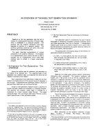
This
information
then
makes
it
possible
to
compute
the
total
diversity,
which
is
worth
1015
=
d(Go,
HyL)
+

d(Go,
Or)
+
d(HyL,
HyS),
and
to
draw
the
corresponding
taxonomic
tree
(figure
1).
The
link
HyS
in
{Go,
Or,
HyL,
HyS}
is
placed
between
the
representative
HyL
and
the

closest
neighbour
Or
of
HyL
in
{Go,
Or,
HyL}.
The
link
Or
in
{Go,
Or,
HyL}
is
then
placed
between
the
representative
Go
and
the
closest
neighbour
HyL
of
Go

in
{Go,
HyL},
resulting
in
a
final
order
of
Go,
Or,
HyS,
HyL.
3.
APPLICATION:
EXAMPLE
OF
EUROPEAN
CATTLE
BREEDS
3.1.
Evaluation
of
diversity
The
Weitzman method
has
been
applied
to

data
collected
by
F.
Grosclaude
[2]
on
biochemical
polymorphisms
(11
blood
group
loci
and
the
locus
of
blood
serum
transferrin
and
that
of
beta-casein)
of
19
European
cattle
breeds,
including

18
French
breeds
and
the
British
Shorthorn.
This
latter
was
included
because
of
its
Durham
ancestor
that
has
been
introduced
in
some
French
regions
during
the
last
century.
The
authors

calculated
the
Nei
standard
distances
considering
the
13
polymorphic
loci
(table
1).
Results
of
the
different
steps
of
the
computations
of
diversity
are
shown
in
table
II.
The
graphical
representation

of
the
result
is
shown
in
figure
2.
A
clear
discrimi-
nation
is
observed
between
two
groups
i.e.
i)
a
first
group
made
of
Northern
dairy
breeds
(Frisonne,
Flamande,
Maine

Anjou,
Shorthorn)
and
ii)
another
group
involv-
ing
beef
and
hardy
breeds
of
the
Center
and
West
part
of
France
(Salers,
Aubrac,
Limousine,
Charolais,
Ferrandaise,
Blonde
d’Aquitaine)
as
well
as

Western
and
Eastern
dual
purpose
breeds
(e.g.
Pie
Rouge,
Abondance,
Tarentaise,
Brune
des
Alpes,
Bretonne
Pie-Noire,
Montb6liarde
and
Parthenaise);
the
original
location
of
the
Normande
breed
between
those
two
groups

as
already
mentioned
by
Grosclaude
et
al.
[2]
should
also
be
noted.
Current
population
sizes
in
some
of
those
breeds
are
so
restricted
that
they
are
said
to
be

endangered:
e.g.
Bretonne
Pie
Noire,
Ferrandaise,
Vosgienne
or
the
Shorthorn.
The
Weitzman
method
allows
us
to
quantify
the
loss
of
diversity
caused
by
the
extinction
of
any
subset
among
the

19
original
breeds.
By
looking
at
the
tree
it
is
evident
that
the
extinction
of
the
Shorthorn
causes
a
much
greater
loss
of
diversity
than
the
extinction
of
the
Flamande,

whose
distance
from
its
closest
neighbour,
the
Frisonne
Pie
Noire,
is
quite
small.
By
computing
the
diversities
of
the
initial
set
of
breeds
and
the
set
minus
the
Flamande,
or

the
Shorthorn,
or
both
the
Flamande
and
the
Shorthorn,
one
finds
that
the
loss
of
the
set
Flamande
+
Shorthorn
induces
a
reduction
of
diversity
equal
to
the
sum
of

the
reductions
caused
by
the
loss
of
each
of
these
breeds.
This
property
of
additivity
is
related
to
the
degree
of
’independence’
between
the
two
breeds.
On
the
other
hand,

if
the
extinctions
of
the
Montb6liarde
and
the
Parthenaise
were
in
The
loss
of
diversity
caused
by
the
extinction
of
a
set
of
breeds
can
be
estimated
by
the
sum

of
the
ordinates
of
the
nodes
that
would
disappear
from
the
tree
if
the
extinct
breeds
were
to
be
removed,
without
any
other
change.
Thus, just
by
looking
at
the
tree,

it
is
obvious
than
the
loss
of
the
Normande
would
decrease
the
diversity
eight
or
nine
times
more
than
the
loss
of
the
Blonde
d’Aquitaine,
and
even
more
than
the

loss
of
a
set
including
Charolaise,
Ferrandaise
and
Blonde
d’Aquitaine.
3.2.
Further
considerations
on
conservation
strategies
The
algorithm
may
be
applied
to
evaluate
the
relative
merit
of
breeds
with
small

or
medium
population
sizes
regarding
diversity.
Let
us
consider
the
whole
set
(say
Q)
of
the
18
French
cattle
breeds
analysed
in
this
study,
and
that
(say
L)
of
the

six
largest
dairy
(Francaise
Frisonne,
Montb6liarde
and
Normande)
and
beef
breeds
(Blonde
d’Aquitaine,
Charolaise
and
Limousine).
The
relative
loss
due
to
keeping
those
six
breeds
only
is
57.2
%.
Now

one
may
ask
which
is
the
most
interesting
breed
to
select
among
the
rest
if
any
of
them
has
to
be
preserved.
This
can
be
evaluated
by
considering
the
relative

loss
of
diversity
between
Q
and
L
plus
each
of
those
12
breeds.
Results
based
on
Nei
and
(Cavalli-Sforza)
distances
are
the
following:
The
breed
providing
the
lowest
loss
of

diversity
is
the
Salers
breed
followed
by
the
Aubrac.
The
ranking
is
consistent
across
the
two
distances
used.
Although
this
is
only
an
illustration
which
would
deserve
further
analysis
including

additional
markers,
this
example
is
a
significant
one
as
those
breeds
have
been
recognized
as
key
hardy
breeds
for
a
long
time
[7].
4.
DISCUSSION
AND
CONCLUSION
The
method
presented provides

several
results
with
different
degrees
of
robust-
ness
and
different
potential
applications.
As
indicated
above,
the
value
of
diversity
possesses
a
useful
property
of
continuity
in
distances.
The
results
may

be
considered
as
relevant
to
support
decisions
affecting
the
breeds
or
species
to
be
preserved.
The
choice
would
be
based
only
on
objective
computations,
without
relying
on
such
subjective
characteristics

as
beauty,
interest
for
future
or
present
generations
or
any
other
intrinsic
criterium.
Experience
has
shown
that
it is
difficult
to
base
priorities
on
such
criteria.
The
Weitzman
approach
to
diversity

allows
further
developments.
Weitzman
[10]
suggests
defining
a
diversity
expected
after
a
given
period
of
time,
based
on
the
extinction
probability
of
each
element
of
the
set
considered.
If n
elements

are
endangered,
2
survival-extinction
patterns
may
occur
with
given
probabilities,
and
for
each
pattern
the
resulting
diversity
may
be
calculated.
Weitzman
then
defines
a
’marginal
diversity’
of
each
element,
obtained

as
the
partial
derivative
of
the
expected
diversity
with
respect
to
the
extinction
probability
of
this
element.
The
marginal
diversity
of
breed
i measures
the
relative
gain
in
expected
diversity
(after

50
years
say)
from
improving
the
survival
probability
of
breed
i.
In
a
similar
fashion,
one
could
assume
that
the
extinction
of
a
breed
can
be
completely
avoided
by
using

cryopreservation
and
calculate
the
gain
in
expected
diversity
obtained
by
cryopreserving
each
endangered
breed.
Knowing
the
pairwise
genetic
distances
and
the
risk
status
of
a
given
set
of
endangered
breeds

as
expressed
through
their
respective
probabilities
of
extinction,
an
order
of
priority
for
a
cryopreservation
programme
could
thus
be
established.
Because
diversity
is
computed
recursively,
it
involves
very
long
calculations

when
the
size n
of
the
set
is
larger
than
25.
The
approximation
proposed
in
this
study
relies
on
a
random
choice of
the
link
at
each
stage
of
the
recursive
algorithm,

i.e.
on
sampling
trees
among
the
2n-1
possible
trees.
The
procedure
can
be
applied
as
follows:
i)
compute
V
among
the
elements
of
S
by
choosing
at
each
step
the

link
not
from
the
formula
in
(6),
but
at
random
out
of
the
pair
of
closest
neighbours,
ii)
repeat
i)
m
times
such
as
to
generate
m
different
values
of

V,
iii)
take
as
the
estimated
value
of
V(S)
the
maximum
value
of
V
over
all
values
computed.
This
can
be
performed
by
choosing
at
random
m
integers
smaller
than

2!!! ,
convert
them
into
their
binary expression
and
use
the
convention
that
the
link
will
be
the
first
element
if
the
value
is
0
and
the
second
if
it
is
1.

This
procedure
was
tested
on
a
set
of
29
cattle
breeds
using
data
from
Moazami-Goudarzi
(pers.
comm.).
For
m
=
10
000,
the
estimated
value
of
V
was
at
least

of
13 200
as
compared
to
a
real
value
of
13
722,
i.e.
bias
lower
than
4
%.
This
approximation
is
quite
good
regarding
the
time
of
computation
required
by
this

estimation
(20
min)
while
the
complete
algorithm
needed
more
than
8
days.
On
the
other
hand,
the
graphical
representation
might
be
sensitive
to
slight
modifications
of
the
distance
matrix
if

the
values
of
diversity
are
close
for
cer-
tain
subsets.
Simulation
procedures
to
evaluate
the
robustness
of
clades
have
been
proposed
by
Weitzman
[8].
Although
the
clustering
power
looks
satisfying

on
the
examples
we
considered,
any
phylogenetic
interpretation
of
the
results
should
be
used
with
caution.
It
should
also
be
emphasized
that
the
use
made
of
genetic
dis-
tances
in

this
approach
differs
from
their
use
in
deriving
genealogical
trees.
Though
trees
are
useful
geometric
representations
of
diversity -
the
diversity
function
de-
fined
above
is
indeed
equal
to
the
total

branch
length
of
the
corresponding
tree -
they
must
be
considered
as
telling
the
evolutionary
story
that
best
fits
the
diversity
observed,
but
not
necessarily
as
telling
the
’true’
story.
In

fact,
as
emphasized
by
Weitzman
[9],
there
is
no
need
for
the
elements
to
have
been
generated
by
any
real
evolutionary
phylogeny.
This
has
to
be
kept
in
mind
particularly

when
sets
of
domestic
breeds
are
considered.
Given
the
exchanges
known
to
have
occurred
in
their
past
histories,
domestic
breeds
are
indeed
not
likely
to have
resulted
from
a
strict
tree-like

branching
process.
Whereas
taxonomists
are
essentially
interested
in
finding
the
evolutionary
story
behind
a
given
observed
diversity,
conservationists,
especially
breed
conservationists,
do
not
need
that
type
of
information
as
they

are
more
concerned
with
the
future
evolution
of
diversity.
The
main
use
of
the
Weitzman method
is
to
determine
preservation
strategies.
It
supposes,
however,
that
the
elements
of
the
set
considered

are
and
remain
distinct.
If
this
constraint
can
be
removed,
it
may
be
suggested
that
certain
endangered
breeds
be
amalgamated
with
other
ones.
The
population
size
would
increase,
no
additional

costs
would
be
engaged,
and
the
direct
loss
of
alleles
that
results
from
an
extinction
could
be
avoided.
Of
course,
this
implies
that
the
breed
standards
should
be
relaxed
for

a
while,
but
it
is
a
dynamic
conception
of
preservation
that
may
offer
interesting
solutions
in
some
cases.
Despite
the
criticisms
which
can
be
raised
against
the
Weitzman
approach,
including

that
it
ignores
the
differences
in
within
unit
variation,
it
should
be
kept
in
mind
that
it
does
satisfy
certain
basic
properties
which
do
not
always
hold
with
traditional
criteria.

The
principle
(1)
of
’monotonicity
in
species’
means
that
the
change
in
diversity
V(SBi) -
V(S)
due
to
the
loss
of
some
population
i
is
always
negative
or
nil
(for
i being

a
twin
element).
In
contrast,
this
property
does
not
apply
to
variance,
for
it
can
be
easily
shown
that
the
total
variance
of
a
mixture
of
populations
can
increase
after

some
of
them
are
deleted.
ACKNOWLEDGMENTS
This
work
was
conducted
while
Caroline
Thaon
was
on
a
’stage
de
fin
d’6tudes’
at
the
Station
de
génétique
quantitative
et
appliqu6e
(SGC!A),
Inra,

Jouy-en-Josas
as
a
student
from
the
Ecole
Polytechnique,
Palaiseau.
She
greatly
acknowledges
the
support
of
both
institutions
in
making
this
stay
feasible.
Special
thanks
are
expressed
to
F.
Grosclaude
and

K.
Moazami-Goudarzi
(Laboratoire
de
génétique
biochimique,
Jouy-en-Josas)
for
providing
the
data
on
cattle
analysed
in
this
study.
We
are
also
grateful
to
C.
Dillmann
and
P.
Dubreuil
(Inra,
Station
de

génétique
vegetale,
Le
Moulon)
and
S.
Lemarié
(Inra-
SERD,
Grenoble)
for
having
provided
additional
test-examples,
and
to
Bruce
Southey
and
an
anonymous
referee
for
their
valuable
comments
which
helped
to

improve
the
manuscrit.
E.
Thompson
is
also
thanked
for
her
English
revision
of
the
text.
REFERENCES
[1]
Cunningham
P.,
Genetic
diversity
in
domestic
animals:
strategies
for
conservation
and
development,
in:

Miller
R.H.,
Pursel
V.G.,
Norman
H.D.
(Eds.),
XX
Biotechnology’s
Role
in
the
Genetic
Improvement
of
Farm
Animals,
American
Society
of
Animal
Science,
Savoy,
IL,
USA,
1996,
pp.
13-23.
[2]
Grosclaude

F.,
Aupetit
R.Y.,
Lefebvre
J.,
Mériaux
J.C.,
Essai
d’analyse
des
relations
génétiques
entre
les
races
bovines
frangaises
à
1’aide
du
polymorphisme
biochimique,
Genet.
Sel.
Evol.
22
(1990)
317-338.
[3]
May

R.M.,
Taxonomy
as
destiny,
Nature
347
(1990)
129-130.
[4]
Ollivier
L.,
Génétique
et
conservation
animales,
in:
Matassino
D.,
Boyazoglu
J.,
Capuccio
A.
(Eds.),
International
Symposium
on
Mediterranean
Animal
Germplasm
and

Future
Human
Challenges,
EAAP
publication
no.
85,
Wageningen
Pers,
Wageningen,
1997,
pp.
211-219.
[5]
Solow
A.,
Polasky
S.,
Broadus
J.,
On
the
measurement
of
biological
diversity,
J.
Environ.
Econom.
Manag.

24
(1993)
60-68.
[6]
Vane-Wright
R.I.,
Humphries
C.J.,
Williams
P.H.,
What
to
protect?
Systematics
and
the
agony
of
choice,
Biol.
Cons.
55
(1991)
235-254.
[7]
Vissac
B.,
Etude
génétique
de

la
race
d’Aubrac,
in:
L’Aubrac,
CNRS,
Paris,
I,
1970,
pp.
29-102.
[8]
Weitzman
M.,
A
reduced
form
approach
to
maximum
likelihood
estimation
of
evolutionary
trees,
Harvard
Institute
of
Economic
Research,

Paper
No.
1569,
1991.
[9]
Weitzman
M.,
On
diversity,
Quart.
J.
Econ.
107
(1992)
363-405.
[10]
Weitzman
M.,
What
to
preserve?
An
application
of
diversity
theory
to
crane
conservation,
Quarter.

J.
Econ.
108
(1993)
157-183.
APPENDIX:
the
maximum
likelihood
tree
Weitzman
[8]
provides
the
following
phylogenetic
interpretation.
Let
us
note
p(i,
j)
the
conditional
probability
P(i! j)
that
a
species
i exists

given
that
a
species
j
exists.
Assume
that
this
probability
is
a
function
of
the
genetic
distance
between
i
and
j.
The
hypothesis
underlying
this
assumption
is
that
the
distance

d(i,
j)
between
two
species
i and j
measures
the
time
since
their
separation.
More
precisely,
we
will
suppose
that
p(i, j)
=
exp
!-ad(i,
j)]
where A
is
a ’universal
extinction
rate’.
The
maximum

likelihood
tree
is
the
evolution
scheme
(i.e.
the
set
of
unknown
ancestors)
which
maximizes
the
probability
that
every
element
of
S
exists
at
the
current
time.
Let
P( j !i)
be
the

conditional
probability
that
species j
exists
given
i
exists.
Assuming
that
the
evolution
scheme
is
known,
it
can
be
shown
that,
for
any
subset
Q
E
S,
and
J
E
SBQ,

the
conditional
probability
P(jlQ)
that j
survived
given
Q
exists
satisfies
Note
p(j,
Q)
=
m! P(j!i).
Now,
from
basic
probability
theory,
P(jlQ) -
t€Q
P(Q
U j)/P(Q),
and
combining
this
with
(A.1)
leads

to:
Let
us
note
11(8),
the
largest
probability
that
S
exists,
i.e.
the
probability
of
existence
under
the
most
favourable
evolution
scheme.
Equation
(A.2)
applied
for
Q
=
SBi,
and j

=
i implies
Any
evolution
scheme
that
would
induce
a
value
of
P(S)
=
II
*
would
be
identified
as
the
scheme
under
which
the
probability
that
S
exists
is
maximal,

ie
the
maximum
likelihood
tree.
Taking
the
logarithm
of
equation
(A.3)
and
normalizing A
to
1,
it
becomes:
Since
(A.5)
has
been
studied
above
and
solved
by
algorithm
(6),
we
are

able
to
exhibit
such
an
evolution
scheme.
The
tree
generated
by
the
Weitzman
method
can
be
interpreted
as
the
maximum
likelihood
tree,
i.e.
the
tree
that
maximizes
the
likelihood
of

the
current
survival
pattern
of
the
species.