Báo cáo khoa hoc:"The PX-EM algorithm for fast stable fitting of Henderson’s mixed model" ppt
Bạn đang xem bản rút gọn của tài liệu. Xem và tải ngay bản đầy đủ của tài liệu tại đây (413.89 KB, 21 trang )
Genet. Sel. Evol. 32 (2000) 143–163 143
c
INRA, EDP Sciences
Original article
The PX-EM algorithm
for fast stable fitting
of Henderson’s mixed model
Jean-Louis FOULLEY
a∗
, David A. VAN DYK
b
a
Station de g´en´etique quantitative et appliqu´ee
Institut national de la recherche agronomique
78352 Jouy-en-Josas Cedex, France
b
Department of Statistics, Harvard University
Cambridge, MA 02138, USA
(Received 7 September 1999; accepted 3 January 2000)
Abstract – This paper presents procedures for implementing the PX-EM algorithm of
Liu, Rubin and Wu to compute REML estimates of variance covariance components
in Henderson’s linear mixed models. The class of models considered encompasses
several correlated random factors having the same vector length e.g., as in random
regression models for longitudinal data analysis and in sire-maternal grandsire models
for genetic evaluation. Numerical examples are presented to illustrate the procedures.
Much better results in terms of convergence characteristics (number of iterations and
time required for convergence) are obtained for PX-EM relative to the basic EM
algorithm in the random regression.
EM algorithm / REML / mixed models / random regression / variance compo-
nents
R´esum´e – L’algorithme PX-EM dans le contexte de la m´ethodologie du mod`ele
mixte d’Henderson.
Cet article pr´esente des proc´ed´es permettant de mettre en
œuvre l’algorithme PX-EM de Liu, Rubin et Wu `a des mod`eles lin´eaires mixtes
d’Henderson. La classe de mod`eles consid´er´ee concerne plusieurs facteurs al´eatoires
corr´el´es ayant la mˆeme dimension vectorielle comme c’est le cas avec les mod`eles de
r´egression al´eatoire dans l’analyse des donn´ees longitudinales ou avec les mod`eles p`ere-
grand-p`ere maternel en ´evaluation g´en´etique. Des exemples num´eriques sont pr´esent´es
pour illustrer ces techniques. L’algorithme PX-EM pr´esente de nettement meilleurs
r´esultats en terme de caract´eristiques de convergence (nombre d’it´erations et temps
de calcul) que l’EM de base sur les exemples ayant trait `a des mod`eles de r´egression
al´eatoire.
algorithme EM / REML / mod`eles mixtes / r´egression al´eatoire / composantes
de variance
∗
Correspondence and reprints
E-mail:
144 J L. Foulley and D.A. van Dik
1. INTRODUCTION
Since the landmark paper of Dempster et al. [4], the EM algorithm has
been among the most popular statistical techniques for calculating parameter
estimates via maximum likelihood, especially in models accounting for missing
data, or in models that can be formulated as such. As explained by Meng
and van Dyk [23], the popularity of EM stems mainly from its computational
simplicity, its numerical stability, and its broad range of applications.
Biometricians, especially those working in animal breeding, have been among
the largest users of EM. Modern genetic evaluation typically relies on best lin-
ear unbiased prediction (BLUP) of breeding values [13,14] and on restricted
(or residual) maximum likelihood (REML) of variance components of Gaus-
sian linear mixed models [12, 27]. BLUP estimates are obtained by solving
Henderson’s mixed model equations, the elements of which are natural compo-
nents of the E-step of the EM algorithm for REML estimation which explains
the popularity of the triple of BLUP-EM-REML.
Unfortunately, the EM algorithm can be very slow to converge in this setting
and various alternative procedures have been proposed: see e.g., Misztal’s
[26] review of the properties of various algorithms for variance component
estimation and Johnson and Thompson [15] and Meyer [25] for a discussion
of a second order algorithm based on the average of the observed and expected
information.
Despite its slow convergence, EM has remained popular, primarily because
of its simplicity and stability relative to alternatives [32]. Thus, much work
has focused on speeding up EM while maintaining these advantages. Rescaling
the random effects which are treated as missing data by EM has been a very
successful strategy employed by several authors; e.g., Anderson and Aitkin [2]
for binary response analysis, Foulley and Quaas [7] for heteroskedastic mixed
models, and Meng and van Dyk [24] for mixed effects models using a Cholesky
decomposition (see also procedures developed by Lindstrom and Bates [17]
for repeated measure analysis and Wolfinger and Tobias [35] for a mixed
model approach to the analysis of robust-designed experiments). To further
improve computational efficiency, the principle underlying the random effects
was generalized by Liu et al. [21] who introduced the parameter expanded EM
or PX-EM algorithm, which in the case of mixed effects models fits the rescaling
factor in the iteration.
The purpose of this paper is twofold: (i) to give an overview of this new
algorithm to the biometric community, and (ii) to illustrate the procedure
with several small numerical examples demonstrating the computational gain of
PX-EM.
The paper is organized as follows into six sections. In Section 2, the
general structure of the models is described and in Section3atypical EM
implementation for these models (called EM
0
for clarity) is reviewed. The
fourth Section briefly introduces the general PX-EM algorithm and gives
appropriate formulae for mixed linear models. Two examples (sire-maternal
grandsire models and random coefficient models) appear in Section 5 and
Section 6 contains a brief discussion.
PX-EM and mixed model methodology 145
2. MODEL STRUCTURE
We consider the class of linear mixed models including K dependent (u
k
;
k =1, 2, ,K) random factors, u
k
for k =1,2, ,K using Henderson’s
notation,
y = Xβ +
K
k=1
Z
k
u
k
+ e (1)
or, in a more compact form
y = Xβ + Zu + e,
where y is the (N × 1) data vector, β isa(p × 1) vector of fixed effects
with matrix X of explanatory discrete or continuous variables, u is a (q
+
× 1)
vector of random effects (q
+
=
K
k=1
q
k
) formed by concatenating the K(q
k
×1)
vectors u
k
, u =(u
1
, u
2
, ,u
k
, ,u
K
)
with corresponding incidence matrix
Z
(N×q
+
)
=(Z
1
, Z
2
, ,Z
k
, ,Z
K
), and e isa(N × 1) vector of residuals.
The usual Gaussian assumption is made for the distribution of (y
, u
, e
)
i.e., y ∼ N(Xβ, ZGZ
+ R) where
G = var (u)={G
k,l
} with G
k,l
=Cov(u
k
, u
l
)=A
kl
g
kl
(2a)
and
R = var(e)=Hσ
2
e
(2b)
In (2a), A
kl
isa(q
k
× q
l
) matrix of known coefficients and g
kl
is a real
parameter known as the (k, l) covariance component such that G
0
= {g
kl
}, the
u-covariance matrix, is positive definite; a similar definition applies to H and
σ
2
e
for the residual variance component.
We assume that all u-components have the same dimension i.e., the same
number of experimental units, q
k
= q for all k, and similarly A
kl
= A for all
k, l, so that G can be written as:
G = G
0
⊗ A, (3)
where ⊗ symbolizes the direct or Kronecker product as defined e.g., in Searle
[31].
Two important models in genetics and biometrics belong to this class of
models.
First, the “sire-maternal grandsire” model (or SMGS model) as described
by Bertrand and Benyshek [3],
y = Xβ + Z
s
u
s
+ Z
t
u
t
+ e, (4)
where u
s
and u
t
refer to (q × 1) vectors of sire and maternal grandsire
contributions of q males respectively and A is the matrix of additive genetic
relationships (or twice Malecot’s kinship coefficients) between those males.
146 J L. Foulley and D.A. van Dik
Here R = Iσ
2
e
, G =
Aσ
2
s
Aσ
st
Aσ
st
Aσ
2
t
= G
0
⊗ A, G
0
=
σ
2
s
σ
st
σ
st
σ
2
t
,
and g
0
=vech(G
0
)=(σ
2
s
,σ
st
,σ
2
t
)
is a function of the variance covariance
components of additive direct and maternal effects of genes.
The second model, a random coefficient model [22], can be applied for
instance to longitudinal data analysis (Diggle et al. [5]; Laird and Ware [16];
Schaeffer and Dekkers [30]), and is usually written as
y
i
= X
i
β +
K
k=1
Z
ik
u
ik
+ e
i
for i =1, 2, ,q
where y
i
=(y
i1
,y
i2
, ,y
ij
, ,y
in
i
)
is the (n
i
× 1) vector of measurements
made on the ith individual (i =1, 2, ,q), X
i
β is the contribution of fixed
effects, and is the kth random regression coefficient (e.g., intercept, linear
slope) on covariate information Z
ik
(e.g., time or age) pertaining to the ith
individual.
Under the general form (1), individuals are nested within random effects
whereas in random coefficient models, the opposite holds, coefficients (factors)
are nested within individuals. That is,
y
i
= X
i
β + Z
i
u
i
+ e
i
for i =1, 2, ,q (5)
with u
i
=(u
i1
, u
i2
, ,u
ik
, ,u
iK
)
, and Z
i(N×K)
=(Z
i1
, Z
i2
, ,Z
ik
, ,
Z
iK
) so that under (5), var(u
i
)=a
ii
G
0
and cov (u
i
, u
i
)=a
ii
G
0
, i.e.,
var (u
1
, u
2
, ,u
i
, ,u
q
)
= A ⊗ G
0
.
Generally, these models assume independence among residuals var(e
i
)=
I
n
i
σ
2
e
and independence among individuals, A = I
q
, but this is neither
mandatory nor always appropriate as e.g., with data recorded on relatives.
Readers may be more familiar with one of the two forms (1) or (5), but both
are obviously equivalent and we may use whichever is more convenient.
3. THE EM
0
ALGORITHM
3.1. Typical procedure
To define an EM algorithm to compute REML estimates of the model
parameter γ =(g
0
,σ
2
e
)
, we hypothesize a complete data set, x, which augments
the observed data, y, i.e. x =(y
, β
, u
)
. As in [4] and [7], we treat β as a
vector of random effects with variance tending to infinity.
Each iteration of the EM algorithm consists of two steps, the expectation
or E step and the maximization or M step. In the Gaussian mixed model,
this separates the computation into two simple pieces. The E-step consists of
taking the expectation of the complete data log likelihood L(γ; x)=lnp(x|γ)
with respect to the conditional distribution of the “missing data”: z =(β
, u
)
vector given the observed data y with γ set at its current value γ
[t]
i.e.,
Q(γ|γ
[t]
)=
L(γ; y, z)p(z|y, γ = γ
[t]
)dz, (6)
PX-EM and mixed model methodology 147
while the M-step updates γ by maximizing (6) with respect to γ i.e.,
γ
[t+1]
= arg max
γ
Q(γ|γ
[t]
). (7)
We begin by deriving an explicit expression for (6) and then derive the two
steps of the EM algorithm. By definition p(x|γ)=p(y|β, u, γ)p(β, u|γ), where
p(y|β, u, γ)=p(y|β, u,σ
2
e
)=p(e|σ
2
e
)
and
p(β, u|γ) ∝ p(u|g
0
),
so that
L(γ; x)=L(σ
2
e
; e)+L(g
0
; u)+const. (8)
Formula (8) allows the formal dissociation of the computations pertaining
to the residual σ
2
e
from the u-components of variance g
0
. Combining (6) with
(8) leads to
Q(γ|γ
[t]
)=Q
e
(σ
2
e
|γ
[t]
)+Q
u
(g
0
|γ
[t]
)+const. (9)
The expressions on the right-hand side can be written explicity
Q
e
(σ
2
e
|γ
[t]
)=−1/2[Nln 2π +ln|H|+ N ln σ
2
e
+ E(e
H
−1
e|y, γ
[t]
)/σ
2
e
] (10)
and,
Q
u
(g
0
|γ
[t]
= −1/2[q
+
ln 2 π +ln|G| + E(u
G
−1
u|y, γ
[t]
)].
Under assumption (3), |G| = |G
0
|
q
|A|
K
and G
−1
= G
−1
0
⊗A
1
,soQ
u
(g
0
|γ
[t]
)
reduces to
Q
u
(g
0
|γ
[t]
)=−1/2[q
+
ln 2π + K ln |A|+ qln|G
0
| +tr(G
−1
0
Ω
[t]
)], (11)
where Ω
[t]
= E{u
k
A
−1
u
l
|y, γ
[t]
} for k, l =1, 2, ,K.
For the M-step, we maximize (10) as a function of σ
2
e
, and (11) as a function
of g
0
.ForH known, this results in
σ
2[t+1]
e
=[E(e
H
−1
e|y, γ
[t]
)]/N (12)
and
G
[t+1]
0
=Ω
[t]
/q, (13)
see Lemma 3.2.2 of Anderson [1], page 62.
The expectations in (12) and (13), i.e. the E-step, can be computed using
elements of Henderson’s [14] mixed model equations (ignoring subscripts), i.e.,
X
H
−1
XX
H
−1
Z
Z
H
−1
XZ
H
−1
Z + σ
2
e
G
−1
ˆ
β
ˆ
u
=
X
H
−1
y
Z
H
−1
y
, (14)
148 J L. Foulley and D.A. van Dik
where
ˆ
β is the GLS estimate of β, and
ˆ
u is the BLUP of u. In particular, we
compute
E(e
H
−1
e|y, γ)=
ˆ
e
H
−1
ˆ
e + σ
2
e
[p + q
+
− σ
2
e
tr (C
uu
G
−1
)], (15)
and
E(u
k
A
−1
u
l
|y, γ)=
ˆ
u
k
A
−1
ˆ
u
l
+ σ
2
e
tr (A
−1
C
u
k
u
l
), (16)
where p = rank(X), q
+
= Kq = dim(u) and C
uu
is the block of the in-
verse of the coefficient matrix of (14) corresponding to u. Further numerical
simplifications can be carried out to avoid inverting the coefficient matrix at
each iteration using diagonalization or tridiagonalization procedures (see e.g.,
Quaas [29]).
3.2. An ECME version
In order to improve computational performance, we can sometimes update
some parameters without defining a complete data set. In particular, the ECME
algorithm [20] suggests separating the parameter into several sub parameters
(i.e. , model reduction), and updating each sub parameter in turn conditional
on the others. For each of these sub parameters, we can maximize either the
observed data log likelihood directly, i.e., L(γ; y) or the expected augmented
data log likelihood, Q(γ|γ
[t]
).
To implement an ECME algorithm in the mixed effects model, we rewrite
the parameter as ζ =(d
0
,σ
2
e
) where var(y)=Wσ
2
e
with W = ZDZ
+ H,
D = D
0
⊗ A, and d
0
= vech(D
0
) and first update σ
2
e
by directly maximizing
L(ζ; y) (without recourse to missing data) under the constraint that d
0
is fixed
at d
[t]
0
σ
2[t+1]
e
=
[y − X
ˆ
β(d
[t]
0
)]
[W(d
[t]
0
)]
−1
[y − X
ˆ
β(d
[t]
0
)]
N − p
.
(17)
An ML analogue of this formula (dividing by N instead of N − p) was first
obtained by Hartley and Rao [12] in their general ML estimation approach
to the parameters of mixed linear models; see also Diggle et al [5], page 67.
Second, we update d
0
by maximizing Q(d
0
,σ
2[t+1]
|ζ
[t]
) using the missing data
approach,
D
[t+1]
0
= G
[t+1]
0
/σ
2[t+1]
e
, (18)
where G
[t+1]
0
is defined in (13).
Henderson [13] showed that the expression for σ
2
e
in (17) can be obtained
from his mixed model equations solutions as
σ
2[t+1]
e
=
[y
H
−1
y −
ˆ
β
[t]
X
H
−1
y −
ˆ
u
[t]
Z
H
−1
y]
N − p
, (19)
where
ˆ
β
[t]
and
ˆ
u
[t]
are defined by (14) evaluated with σ
2
e
G
−1
= D
−1
computed
using d
[t]
0
. Incidentally, this shows that the algorithm developed by Henderson
[14] to compute REML estimates, as early as 1973, introduces model reduction
in a manner similar to recent EM-type algorithms.
PX-EM and mixed model methodology 149
4. THE PX-EM ALGORITHM
4.1. Generalities
In the PX-EM algorithm proposed by Liu et al. [21], the parameter space of
the complete data model is expanded to a larger set of parameters, Γ =(γ
∗
, α),
with α a working parameter, such that (γ
∗
, α) satisfies the following two
conditions:
– it can be reduced to the original parameter γ, maintaining the observed
data model via a many-to-one reduction form γ = R(Γ);
– when α is set to its reference (or “null” ) value, (γ
∗
, α
0
) induces the same
complete data model as with γ = γ
∗
i.e., p[x|Γ =(γ
∗
, α
0
)] = p[x|γ = γ
∗
].
We introduce the working parameter because the original EM (EM
0
) imputes
missing data under a wrong model, i.e., the EM iterate γ
[t]
EM
is different from
the MLE. The PX algorithm takes advantage of the difference between the
imputed value α
[t+1]
of α and its reference value α
0
to make what Liu et al.
[21] called a covariance adjustment in γ, i.e.,
γ
[t+1]
X
− γ
[t+1]
EM
≈ b
γ|α
(α
[t+1]
− α
0
) (20)
where γ
[t]
X
is the PX-EM value at iteration [t], γ
[t]
EM
is the EM iterate, and
b
γ|α
is a correction factor. Liu et al. [21] show that this adjustment necessarily
improves the rate of convergence of EM generally in terms of the number of
iterations required for convergence.
Operationally, the PX-EM algorithm, like EM, consists of two steps. In
particular, the PX-E step computes the conditional expectation of the log
likelihood of x given the observed data y with Γ
[t]
set to (γ
[t]
∗
, α = α
0
) i.e.,
Q(Γ|Γ
[t]
)=E[L(Γ; x)|y, Γ
[t]
=(γ
[t]
∗
, α = α
0
)]. (21)
The PX-M step then maximizes (21) with respect to the expanded parame-
ters
Γ
[t+1]
= arg max
Γ
Q(Γ|Γ
[t]
), (22)
and γ is updated via γ
[t+1]
= R(Γ
[t+1]
).
In the next section, we illustrate PX-EM in the Gaussian linear model. In
particular, we will describe a simple method of introducing a working parameter
into the complete data model.
4.2. Implementation of PX-EM in the mixed model
We begin by defining the working parameter as a (K × K) invertible real
matrix α = {α
kl
} which we incorporate into the model by rescaling the random
effects
˜
U = α
−1
U where U
(K×q)
=(u
1
, u
2
, u
k
, ,u
K
)
i.e.,
y = Xβ +
K
k=1
Z
k
u
k
+ e
u
k
=
K
l=1
α
kl
˜
u
l
(23a)
150 J L. Foulley and D.A. van Dik
or alternatively, under (5)
y
i
= X
i
β + Z
i
α
˜
u
i
+ e
i
. (23b)
By the definition of
˜
u
i
,wehave
˜
u
i
∼ N (0, G
0
∗
), where G
0
∗
= α
−1
G
0
(α
−1
)
.
Rescaling the random effects by α introduces the working parameters into two
parts of the model, into (23) and into the distribution of
˜
u
i
which can be viewed
as an extended parametric form of the distribution of u
i
(see (2a)) i.e., when
α = α
0
= I
K
, u
i
and
˜
u
i
have the same distribution.
To understand why the PX-EM works in this case, recall that the REML
estimate is the value of which maximizes
L(γ; y)=
p(y|β, u, γ)p(u|γ)dβdu. (24a)
What is important here is that for any value of α, L(γ; y)=L(γ
∗
, α; y) with
L(γ
∗
, α; y)=
p(y|β,
˜
u, γ
∗
, α)p(
˜
u|γ
∗
)dβd
˜
u. (24b)
Thus, we can fix α in (24b) to be any value at each iteration. Liu et al.
[21] showed that fitting α in the iteration can improve the computational
performance of the algorithm.
Computationally, the PX-EM algorithm replaces the integrand of (24a) with
that of (24b). In particular, in the E-step, we compute Q(Γ|Γ
[t]
)=(γ
[t]
∗
, α =
α
0
). Here we choose α = α
0
, since any value of α will work and using
α
0
reduces computations to those of the EM
0
algorithm. In the M-step, we
update Γ by maximizing Q(Γ|Γ
[t]
), i.e. we compute g
[t+1]
0
∗
= vec(G
[t+1]
0
∗
), α
[t+1]
and σ
2[t+1]
e
∗
. Finally, we reduce these parameter values to those of interest,
G
[t+1]
0
= α
[t+1]
G
[t+1]
0
∗
(α
[t+1]
)
and σ
2[t+1]
e
= σ
2[t+1]
e
∗
(in the remainder of the
paper we fix σ
2
e
∗
at σ
2
e
). We now move to the details of these computations.
In order to derive Q(Γ|Γ
[t]
, we note that
p(y, β,
˜
u|g
0
∗
, α,σ
2
e
) ∝ p(y|β,
˜
u, α,σ
2
e
)p(
˜
u|g
0
∗
),
and
L(Γ|x)=L(α,σ
2
e
|e)+L(g
0
∗
|
˜
u)+const. (25)
thus
Q(Γ|Γ
[t]
)=Q
e
(α,σ
2
e
|Γ
[t]
)+Q
u
(g
0
∗
|Γ
[t]
)+const. (26)
where Γ =(g
0
∗
, (vec α)
,σ
2
e
)
, and Γ
[t]
=(g
[t]
0
∗
, (vec α
0
)
,σ
2[t]
e
)
.
Maximizing Q
u
(g
0
∗
|Γ
[t]
) with respect to g
0
∗
is identical to the corresponding
calculations for g
0
in EM
0
i.e., we set G
[t+1]
0
∗
= Ω
[t]
/q, where Ω
[t]
is evaluated
as in EM
0
with (16).
PX-EM and mixed model methodology 151
Next, we wish to maximize Q
e
(α,σ
2
e
∗
|Γ
[t]
), which can be written formally as
in (10) but with e defined in (23a) or (23b). Partial derivatives of this function
with respect to α are given by:
∂Q
∂α
kl
=
1
σ
2
e
I
i=1
E
u
i
∂α
∂α
kl
Z
i
H
−1
i
(y
i
− X
i
β − Z
i
α
˜
u
i
)|y, Γ
[t]
.
Solving these K
2
equations does not involve σ
2
e
, and is equivalent to solving
the linear system F(vec α
)=h,
K
m=1
K
n=1
f
[t]
kl,mn
α
[t+1]
mn
= h
[t]
kl
; for k, l =1, 2, ,K (27)
where
f
[t]
kl,mn,
=tr[Z
k
H
−1
Z
m
E(u
n
u
l
|y, Γ
[t]
)]] (28)
and
h
[t]
kl
=tr
Z
k
H
−1
E[(y − Xβ)u
l
|y, Γ
[t]
]
. (29)
Explicit expressions for the coefficients when K = 2 are given in Appendix A.
We can compute α
[t+1]
using Henderson’s [14] mixed model equations (14),
suppressing the superscript [t], as follows
f
kl,mn
=tr[Z
k
H
−1
Z
m
(
ˆ
u
n
ˆ
u
l
+ σ
2
e
C
u
n
u
l
)], (30)
h
kl
=
ˆ
u
l
Z
k
H
−1
y − tr
Z
k
H
−1
X(
ˆ
β
ˆ
u
l
+ σ
2
e
C
βu
l
)
, (31)
where Z
k
H
−1
Z
m
is the block of the coefficient matrix corresponding to u
k
and
u
m
; Z
k
H
−1
X is the block corresponding to u
k
and β; C
u
k
u
m
and C
u
k
β
= C
βu
k
are the corresponding blocks in the inverse coefficient matrix; Z
k
H
−1
y is the
sub vector in the right hand side of (14) corresponding to u
k
; and
ˆ
β and
ˆ
u
k
are the solutions for β and u
k
in (14). Once we obtain α
[t+1]
, we update G
0
as indicated previously.
Finally to update σ
2
e
, we maximize Q
e
(α,σ
2
e
|Γ
[t]
) via
σ
2[t+1]
e
= E(e
H
−1
e|y, Γ
[t]
)/N, (32)
where the residual vector, e, is adjusted for the solution α
[t+1]
in (27), i.e.,
using y
i
−X
i
β −Z
i
α
[t+1]
˜
u
i
. A short-cut procedure implements a conditional
maximization with α fixed at α
[t]
= I
K
and results in formula (15) as in the
EM
0
procedure. One can also derive a parameter expanded ECME algorithm
by applying Henderson’s formula (19) with d
0
fixed at d
[t]
0
; see van Dyk [32].
152 J L. Foulley and D.A. van Dik
5. NUMERICAL EXAMPLES
5.1. Description
In this section, we illustrate the procedures and their computational ad-
vantage relative to more standard methods using two sire-maternal grandsire
(model 4) and two random coefficient (model 5) examples.
5.1.1. Sire-maternal grandsire models
The two examples in this section are based on calving score of cattle [6].
From a biological viewpoint, parturition difficulty is a typical example of a
trait involving direct effects of genes transmitted by parents on offspring, and
maternal effects influencing the environmental conditions of the foetus during
gestation and at parturition. Thus, statistically we must consider the sire and
the maternal grandsire contributions of a male, not as simple multiples of each
other (i.e., the first twice that of the second), but as two different but correlated
variables. This model can be written as
y
ijklm
= µ + α
i
+ β
j
+ s
k
+ t
l
+ e
ijklm
, (33)
where µ is an overall mean; α
i
, β
j
are fixed effects of the factors A = sex (i =1, 2
for bull and heifer calves respectively) and B = parity of dam (j =1, 2 and 3
for heifer, second and third calves respectively); s
k
is the random contribution
of male k as a sire and t
l
that of male l as maternal grandsire, and e
ijklm
are
residual errors, assumed iid- N(0,σ
2
e
).
Letting s = {s
k
} and t = {t
l
}, it is assumed that var(s)=Aσ
2
s
, var(t)=
Aσ
2
t
and cov(s, t
)=Aσ
st
, where A is the matrix of genetic relationships
among the several males occurring as sires and maternal grandsires and
g
0
=(σ
2
s
,σ
st
,σ
2
t
)
is the vector of variance-covariance components.
We analyse two data sets; the first is the original data set presented in [6],
which we refer to as “Calving Data 1 or CD1”, and the second is a data set
with the same design structure but with smaller subclass size and simulated
data which we refer to as “Calving Data 2 or CD2” (see Append. B1)
5.1.2. Random coefficient models
Growth data: We first analyse a data set due to Pothoff and Roy [28] which
contains facial growth measurements recorded at four ages (8, 10, 12 and 14
years) in 11 girls and 16 boys. There are nine missing values, which are defined
in Little and Rubin [19]. The data appear in Verbeke and Molenberghs [33]
(see Table 4.11, page 173 and Appendix B2) with a comprehensive statistical
analysis.
We consider model 6 of Verbeke and Molenberghs which is a typical random
coefficient model for longitudinal data analysis with an intercept and a linear
slope, and can be written as
y
ijk
= µ + α
i
+ β
i
t
j
+ a
ik
+ b
ik
t
j
+ e
ijk
, (34)
PX-EM and mixed model methodology 153
where the systematic component of the outcome y
ijk
involves an intercept µ+α
i
varying according to sex i (i =1, 2 for female and male children respectively)
and a linear increase with time (t
j
= 8, 10, 12 and 14 years); the rate β
i
also varies with sex. The a
ik
and b
ik
are the random homologues of α
i
and
β
i
but are defined at the individual level (indexed k within sex i). Letting
u
ik
=(a
ik
,b
ik
)
, it is assumed that the u
ik
’s are iid- N(0, G
0
). Similarly,
letting e
ik
=(e
i1k
,e
i2k
,e
i3k
,e
i4k
)
the e
ik
are assumed iid- N(0,σ
2
e
I
4
) and
distributed independently from the u
ik
’s.
Ultrafiltration data: In our second random coefficient model, we consider
the ultrafiltration response of 20 membrane dialysers measured at 7 different
transmembrane pressures with an evaluation made at 2 different blood flow
rates. These data due to Vonesh and Carter [34] are described and analysed
in detail in the SAS manual for mixed models (Littell et al. [18]; data set 8.2
DIAL Appendix 4, pages 575-577 ; Appendix B3).
Using notations similar to the model for the growth data, we write
y
ijk
= µ + α
i
+
4
r=1
β
r
x
r
ijk
+ a
ik
+
2
r=1
b
r,ik
x
r
ijk
+ e
ijk
, (35)
where y
ijk
is the ultrafiltration rate in ml · h
−1
, µ + α
i
the intercept for
blood rate i (i = 1, 2 for 200, 300 dl·min
−1
),
4
r=1
β
r
x
r
ijk
is the regression of
the response on the transmembrane pressure x
ijk
(dm Hg) as a homogeneous
quartic polynomial; a
ik
and b
r,ik
represent the random coefficients up to the
second degree of the regression defined at the dialyser level (k =1, 2, , 20).
Again, letting u
ik
=(a
ik
,b
1,ik
,b
2,ik
)
and e
ik
= {e
ijk
}, it is assumed that
the u
ik
’s are iid- N(0, G
0
) and the e
ik
’s are iid- N(0,σ
2
e
I
7
) and distributed
independently of each other.
5.2. Calculations and results
REML estimates of variance-covariance parameters were computed for each
of these four data sets using the EM
0
and PX-EM procedures including the
complete (PX-C) and the triangular (PX-T) working parameter matrices, (see
van Dyk [32] for discussion of the use of a lower triangular matrix as the
working parameter). For each of the three EM-type algorithms, the standard
procedure described in this paper was applied as well as those based on
Henderson’s formula for the residual variance. The iteration stopped when the
norm
i
∆θ
2
i
/
i
θ
2
i
of both g
0
and of σ
2
e
, was smaller than 10
−8
.
Results are summarized in Tables I and II for sire-maternal grandsire
(SMGS) and random coefficient (RC) models, respectively. In all cases, the
number of iterations required for convergence was smaller for the PX-C
procedure than for the EM
0
procedure. The decrease in this number of
iterations was 15 to 20% for SMGS models and as high as 70% for RC models.
154 J L. Foulley and D.A. van Dik
Table I. Performance of EM algorithms for estimating variance components in sire
and maternal grandsire models.
Examples
1
Algorithms
2
Calving data I Calving data II
−2L
3
Iterations
4
Time
5
−2L
3
Iterations
4
Time
5
EM
0
a 1760.284442 122 5
746.6163445 627 25
b 1760.284442 123 4
746.6163444 628 22
PX-C a 1760.284442 98 12
746.6163444 533 1’05
b 1760.284442 98 9
746.6163444 534 1’03
PX-T a 1760.284442 104 13
746.6163445 586 1’13
b 1760.284442 104 12
746.6163444 586 1’09
1
Examples: Calving data I: Foulley [6]; Calving difficulty score shown in appendix
B1. Calving data II: same design structure, 4 scores, small progeny group size and
simulated data.
2
Algorithms: EM
0
: Model 0 and PX-C: PX EM with extended and complete
parameters as defined in Liu et al. [21]. PX-T: PX EM with triangular matrix of
parameters as defined by van Dyk [32].
a) standard procedure; b) using Henderson’s formula for residual variance.
3
−2L = minimum of minus twice the restricted log likelihood. Estimates of param-
eters are:
Large pgs: residual = 0.50790017; sire var = 0.03201508; sire mgs covar = 0.01146468;
mgs va = 0.06304075.
Small pgs: residual = 0.852018; sire var = 0.704462; sire mgs covar = 0.533585; mgs
va = 0.923661.
4
Iterations up to convergence for a norm of both the residual variance and the matrix
of u components of variance lower than or equal to 10
−8
.
5
Time to convergence based on an APL2 programme (Dyalog73) run on a PC
Pentium I (90 MHz).
The absolute numbers of iterations were 64 vs. 224 for PX-C vs. EM
0
for growth
data and 76 vs. 259 for the ultrafiltration data.
Since computing time per iteration is larger for PX-C than for EM
0
, the total
computing time remains smaller with EM
0
for the CD1 and CD2 examples.
However, in the RC models, computing time is about halved in both examples.
This impressive advantage of PX-C vs. EM
0
was also observed at different norm
values (10
−6
,10
−9
) and with a different stopping rule (decrease in -2L equal
to or smaller than 10
−8
); see also the plot of EM sequences for the intercept
variance in the “growth data” example (Fig. 1) and for all the u-components
of variance in the ultrafiltration data example (Fig. 2).
PX-EM and mixed model methodology 155
Table II. Performance of EM algorithms for estimating variance components in
random coefficient models.
Examples
1
Algorithms
2
Growth data (1st degree) Ultrafiltration data (2nd degree)
−2L
3
Iterations
4
Time
5
−2L
3
Iterations
4
Time
5
EM
0
a 842.3559004 224 1’07
645.8495069 259 2’30
b 842.3559008 241 1’04
645.8495097 264 2’01
PX-C a 842.3559007 64 32
645.8495076 76 1’18
b 842.3559007 67 31
645.8495062 75 1’19
PX-T a 842.3559007 92 44
645.8495083 352 5’57
b 842.3559007 96 43
645.8495096 372 5’57”
1
Examples: Growth data from Pothoff and Roy [28] with the 9 missing values defined
by Little and Rubin [19]: see also Verbeke and Molenberghs [33] for a detailed analysis.
Here 1st degree polynomial for the random part (intercept + slope). Ultrafiltration
rates of 20 membrane dialyzers measured at 7 pressures and using two blood flood
rates [18, 34]. Here, second degree polynomial for the random part.
2
Algorithms: EM
0
: Model 0 and PX-C: PX EM with extended and complete
parameters as defined in Liu et al. [21]. PX-T: PX EM with triangular matrix of
parameters as defined by van Dyk [32].
a) standard procedure; b) using Henderson’s formula for residual variance.
3
−2L = minimum of minus twice the restricted loglikelihood Estimates of parame-
ters are:
Growth data (original values × 100): residual = 176.6555; (00) = 835.5160; (01) =
−46.5266, (11) = 4.4150.
Ultrafiltration data: residual = 3.317524; (00) = 2.246091; (01) = −3.731253; (02) =
0.687083; (11) = 24.080699; (12) = −6.829680; (22) = 2.172312
0, 1, 2 stand for intercept, first and second degree random coefficient effects respec-
tively.
4
Iterations up to convergence for a norm of both the residual variance and the matrix
of u components of variance lower or equal to 10
−8
.
5
Time to convergence based on an APL2 programme (Dyalog73) run on a PC
Pentium I (90 Mhz).
Results obtained with PX-T were consistently poorer than with PX-C and
in the case of ultrafiltration data even poorer than EM
0
. Computation for this
model is especially demanding because of an adjustment of a second degree
polynomial with a very high absolute correlation between the first and second
degree coefficients of 0.94.
Finally, no practical differences were observed between the standard and the
ECME procedures; Henderson’s formula can be used in practice to compute
the residual variance.
156 J L. Foulley and D.A. van Dik
Figure 1. Two typical sequences of EM iterates for the “growth data” example.
a) starting values: residual = total variance; (00) = 500, (01) = 0, (11) = 5.
b) starting values: residual = 0.5 total variance; (00) = 2000, (01) = 0, (11) = 20.
6. DISCUSSION-CONCLUSION
This paper shows that the PX-EM procedure can be easily implemented
within the framework of Henderson’s mixed model equations. Changes to the
EM
0
procedure are simple requiring only the solution of a (K
2
× K
2
) linear
system at each iteration with K generally 2, 3 or 4. In particular, the PX-
EM procedure can handle the situation of random effects correlated among
experimental units (e.g., individuals) as it often occurs in genetics.
PX-EM and mixed model methodology 157
Figure 2. EM iterates for the “ultrafiltration data” example.
a, b, c, d, e and f stand for (00), (11), (22), (01), (02) and (12) u-components
of variance and covariance respectively; starting values: residual = 4; (00) = (11) =
(22) = 4, (01) = 2, (02) = −1.2, (12) = −2.4.
A ML extension of the PX-EM procedure is straightforward with an appro-
priate change in the conditional expectations of u
k
u
l
and βu
k
along the lines
proposed by Foulley et al. [8] and van Dyk [32].
Our examples confirm the potential advantage of the PX-EM procedure for
mixed linear models already advocated by Liu et al. [21] and van Dyk [32]. The
improvement was especially decisive in the case of random coefficient models.
This is important in practice since these models are becoming more and more
popular among biometricians e.g., epidemiologists and geneticists involved in
the analysis of longitudinal data and space-time phenomena.
158 J L. Foulley and D.A. van Dik
In this manuscript, emphasis was on EM procedures and ways to improve
them. This does not preclude using alternative algorithms for computing maxi-
mum likelihood estimations of variance component e.g. the Average Information
(AI)-REML (Gilmour, Thompson and Cullis [10]).
Nonetheless, EM procedures have two important features:
(i) they allow separation of the computations required for the R matrix
(errors but also time or space processes) and the G matrix for which the PX
version turns out to perform especially well; here we suppose the elements of
H in R fixed but the EM procedure can be easily extended to parameters in
an unknown H [9];
(ii) (PX)EM generally selects the correct sub model when estimates are
on or near the boundary of the parameter space, a property that second order
algorithms do not always exhibit (e.g., the analysis of the growth data in Foulley
et al [9] and the simulations in Meng and van Dyk [24] and van Dyk, [32]).
Actually, this is an example of the well-known stable convergence of EM
type algorithms (i.e., monotone convergence) which second order algorithms
do not generally exhibit [32].
ACKNOWLEDGEMENTS
David van Dyk gratefully acknowledges funding for this project partially
provided by the National Science Foundation (USA) grant DMS-97-05157 and
the US Bureau of the Census. Thanks are also expressed to Christ`ele Robert-
Grani´e and Barbara Heude for their help in the numerical validation of the
growth and ultrafiltration examples via SAS proc mixed.
REFERENCES
[1] Anderson T.W., An introduction to multivariate statistical analysis, J. Wiley
and Sons, New York, 1984.
[2] Anderson D.A., Aitkin M.A., Variance component models with binary re-
sponse: interviewer variability, J. R. Stat. Soc. B 47 (1985) 203–210.
[3] Bertrand J.K., Benyshek L.L., Variance and covariance estimates for mater-
nally influenced beef growth traits. J. Anim. Sci. 64 (1987) 728–734.
[4] Dempster A.P., Laird N.M., Rubin D.B., Maximum likelihood from incom-
plete data via the EM algorithm, J. R. Stat. Soc. B 39 (1977) 1–38.
[5] Diggle P.J., Liang K.Y., Zeger S.L., Analysis of longitudinal data, Oxford
Science Publications, Clarendon Press, Oxford, 1994.
[6] Foulley J.L., Heteroskedastic threshold models with applications to the anal-
ysis of calving difficulties, Interbull Bulletins 18 (1998) 3–11.
[7] Foulley J.L., Quaas R.L., Heterogeneous variances in Gaussian linear mixed
models, Genet. Sel. Evol. 27 (1995) 211–228.
[8] Foulley J.L., Quaas R.L., Than d’Arnoldi C., A link function approach to
heterogeneous variance components, Genet. Sel. Evol. 30 (1998) 27–43.
[9] Foulley J.L., Jaffrezic F., Robert-Grani´e C., EM-REML estimation of covari-
ance parameters in Gaussian mixed models for longitudinal data analysis, Genet. Sel.
Evol. 32 (2000), 129-141.
PX-EM and mixed model methodology 159
[10] Gilmour A.R., Thompson R, Cullis B.R., Average information REML: an
efficient algorithm for variance component parameter estimation in linear mixed
models, Biometrics 51 (1995) 1440–1450.
[11] Hartley H.O., Rao J.N.K., Maximum likelihood estimation for the mixed
analysis of variance model, Biometrika 54 (1967) 93–108.
[12] Harville D.A., Maximum likelihood approaches to variance component esti-
mation and related problems, J. Am. Stat. Assoc. 72 (1977) 320–338.
[13] Henderson C.R., Sire evaluation and genetic trends, in: Proceedings of the
animal breeding and genetics symposium in honor of Dr J Lush, American society of
animal science-American dairy science association, Champaign, 1973, pp. 10-41.
[14] Henderson C.R., Applications of linear models in animal breeding, University
of Guelph, Guelph, 1984.
[15] Johnson D.L., Thompson R., Restricted maximum likelihood estimation of
variance components for univariate animal models using sparse matrix techniques and
average information, J. Dairy Sci. 78 (1995) 449–456.
[16] Laird N.M., Ware J.H., Random effects models for longitudinal data, Bio-
metrics 38 (1982) 963–974.
[17] Lindstr¨om M.J., Bates D.M., Newton-Raphson and EM algorithms for linear
mixed effects models for repeated measures data, J. Am. Stat. Assoc. 83 (1988) 1014–
1022.
[18] Littell R.C., Milliken G.A., Stroup W.W., Wolfinger R.D., SAS System for
mixed models, SAS Institute Inc, Cary, NC, USA, 1996.
[19] Little R.J.A., Rubin D.B., Statistical analysis with missing data, J. Wiley
and Sons, New York, 1977.
[20] Liu C., Rubin D.B., The ECME algorithm: a simple extension of EM and
ECM with fast monotone convergence, Biometrika 81 (1994) 633–648.
[21] Liu C., Rubin D.B.,Wu Y.N., Parameter expansion to accelerate EM: The
PX- EM algorithm, Biometrika 85 (1998) 755–770.
[22] Longford N.T., Random coefficient models, Clarendon Press, Oxford, 1993.
[23] Meng X.L., van Dyk D.A., The EM algorithm - an old song sung to a fast
new tune (with discussion), J. R. Stat. Soc. B 59 (1997) 511–567.
[24] Meng X.L., van Dyk D.A., Fast EM-type implementations for mixed effects
models, J. R. Stat. Soc. B 60 (1998) 559–578.
[25] Meyer K., An average information restricted maximum likelihood algorithm
for estimating reduced rank genetic covariance matrices or covariance functions for
animal models with equal design matrices, Genet. Sel. Evol. 29 (1997) 97-116.
[26] Misztal I., Comparison of computing properties of derivative and derivative-
free algorithms in variance component estimation by REML, J. Anim. Breed. Genet.
111 (1994) 346–352.
[27] Patterson H.D., Thompson R., Recovery of interblock information when
block sizes are unequal, Biometrika 58 (1971) 545–554.
[28] Pothoff R.F., Roy S.N., A generalized multivariate analysis of variance model
useful especially for growth curve problems, Biometrika 51 (1964) 313–326.
[29] Quaas R.L., REML Note book, Mimeo, Cornell University, Ithaca, New York,
1992.
[30] Schaeffer L.R., Dekkers J.C.M., Random regressions in animal models for
test-day production in dairy cattle, in: Proceedings of the 5th World Congress on
Genetics Applied to Livestock Production 18 (1994) 443–446.
[31] Searle S.R., Matrix algebra useful for statistics, John Wiley & Sons, New
York, 1982.
[32] van Dyk D.A., Fitting mixed-effects models using efficient EM-type algo-
rithms, J. Comp. Graph. Stat. (2000) accepted.
160 J L. Foulley and D.A. van Dik
[33] Verbeke G., Molenberghs G., Linear mixed models in practice, Springer
Verlag, New York, 1997.
[34] Vonesh E.F., Carter R.L., Mixed-effects non linear regression for unbalanced
repeated measures, Biometrics 48 (1992) 1–17.
[35] Wolfinger R.D., Tobias R.D., Joint estimation of location, dispersion, and
random effects in robust design, Technometrics 40 (1998) 62–71.
Appendix A
Explicit expression of the system F(vec α
)=h.
The system to be solved has the general form
K
m=1
K
n=1
f
[t]
kl,mn
α
[t+1]
mn
= h
[t]
kl
for k, l =1, 2, ,K
where
f
[t]
kl,mn
=tr[Z
k
H
−1
Z
m
E(u
n
u
l
|y, Γ
[t]
)]
h
[t]
kl
=tr
Z
k
H
−1
E[(y − Xβ)u
l
|y, Γ
[t]
]
Let T
kl
= Z
k
H
−1
Z
l
, and v
k
(q×1)
= Z
k
H
−1
(y − Xβ
) and E
c
(.) designate a
conditional expectation given y, Γ
[t]
, the left hand side wich is symmetric can
be expressed, for K = 2, as:
11 12 21 22
11 E
c
(u
1
T
11
u
1
) E
c
(u
1
T
11
u
2
) E
c
(u
1
T
12
u
1
) E
c
(u
1
T
12
u
2
)
12 E
c
(u
2
T
11
u
2
) E
c
(u
2
T
12
u
1
) E
c
(u
2
T
12
u
2
)
21 E
c
(u
1
T
22
u
1
) E
c
(u
1
T
22
u
2
)
22 E
c
(u
2
T
22
u
2
)
and the right hand side as:
11 12 21 22
E
c
(u
1
v
1
) E
c
(u
2
v
1
) E
c
(u
1
v
2
) E
c
(u
2
v
2
)
PX-EM and mixed model methodology 161
Appendix B
B1. Data sets for sire and maternal grandsire models.
No Environment Genetic factors Calving data I Calving data II
ab s t [1] [2] [3] [1] [2] [3] [4]
1 11 1 4 2327138670
212 1 4 14212211341
3 11 1 7 20166 6611
4 12 1 7 1353 2500
5 12 1 8 954 0420
6 11 2 6 618120408
7 11 2 7 1353 4210
8 1 2 2 8 39105 413110
9 21 2 8 51264 7659
10 22 3 5 885 0034
11 2 1 3 5 16 24 17 0 5 2 12
12 22 3 5 14133 0226
13 2 3 3 2 60 37 14 10 1 1 25
14 22 3 2 22134 1147
15 2 3 4 7 27 9 3 10 3 0 0
16 23 4 8 954 3102
17 2 2 4 9 30 19 8 0 0 6 13
18 22 4 5 23112 6510
Calving data I: Foulley [6]. Calving performance scored according to an increasing
level of dystocia as factors of a = sex, b = age of dam, s = sire of calf and t =
maternal grandsire of calf.
Calving data II: Same design structure with 4 score values, smaller subclass numbers
and simulated data.
a,b,s,t: stand for factors a, b (fixed) and sire and maternal grandsire (random)
respectively. Non-zero elements (i, j)=(j, i) of the numerator relationship matrix
are: (1, 2)=(8, 9)=1/4; (1, 5)=(2, 5)=(3, 7)=(4, 6)=(8, 10)=(9, 10) =
1/2; (i, i) = 1, for any i =1, 2, ,10.
162 J L. Foulley and D.A. van Dik
B2. Growth measurements in 11 girls and 16 boys (from Pothoff and Roy [28];
Little and Rubin [19]).
Age (years) Age (years)
Girl 8 10 12 14 Boy 8 10 12 14
1 210 200 215 230 1 260 250 290 310
2 210 215 240 255 2 215 230 265
3 205 245 260 3 230 225 240 275
4 235 245 250 265 4 255 275 265 270
5 215 230 225 235 5 200 225 260
6 200 210 225 6 245 255 270 285
7 215 225 230 250 7 220 220 245 265
8 230 230 235 240 8 240 215 245 255
9 200 220 215 9 230 205 310 260
10 165 190 195 10 275 280 310 315
11 245 250 280 280 11 230 230 235 250
12 215 240 280
13 170 260 295
14 225 255 255 260
15 230 245 260 300
16 220 235 250
Distance from the centre of the pituary to the pteryomaxillary fissure (unit 10
−4
m).
PX-EM and mixed model methodology 163
B3: Ultrafiltration data set (from [18, 33]).
# QB TMP UFR # QB TMP UFR # QB TMP UFR # QB TMP UFR
2 240 645 2 260 3660 3 255 3885 3 235 1170
2 505 20115 2 500 16950 3 500 19155 3 485 17685
2 995 38460 2 1020 36090 3 980 37650 3 1025 39705
1 2 1485 44985 6 2 1490 42630 11 3 1490 47895 16 3 1515 52680
2 2020 51765 2 1990 46470 3 2015 54495 3 1990 61800
2 2495 46575 2 2480 46275 3 2510 53175 3 2510 61485
2 2970 40815 2 2995 43980 3 2980 59355 3 3020 61425
2 240 3720 2 305 9825 3 280 5715 3 285 1500
2 540 18885 2 505 21630 3 505 20505 3 520 15405
2 995 34695 2 980 42270 3 1000 39405 3 1005 32520
2 2 1475 40305 7 2 1505 50280 12 3 1490 50100 17 3 1500 42435
2 2000 44475 2 2005 45510 3 2000 55155 3 1985 48570
2 2500 42435 2 2505 44250 3 2505 61185 3 2490 53685
2 3010 44655 2 2990 42300 3 3020 50715 3 2995 53655
2 245 2985 2 305 9480 3 355 10410 3 295 6420
2 480 17700 2 505 21750 3 480 19320 3 515 20250
2 1010 35295 2 995 37230 3 1025 43770 3 1010 43050
3 2 1505 41955 8 2 1500 44430 13 3 1500 51225 18 3 1480 58110
2 2000 47610 2 1990 42165 3 1990 58095 3 2000 61995
2 2515 44730 2 2480 43065 3 2500 54090 3 2480 60915
2 2970 46035 2 3000 36615 3 3005 62010 3 3005 63600
2 255 3930 2 250 1560 3 235 3600 3 290 4050
2 495 19830 2 495 16650 3 480 20490 3 495 16590
2 995 40425 2 1000 34530 3 1010 41880 3 1015 40515
4 2 1480 52260 9 2 1500 43815 14 3 1490 49995 19 3 1520 52845
2 1995 49395 2 1965 48495 3 1990 57675 3 2020 60435
2 2490 45975 2 2485 47520 3 2480 62475 3 2500 64830
2 3030 41910 2 2980 41640 3 3005 62145 3 2975 63825
2 255 3210 2 235 1230 3 260 1890 3 400 10935
2 515 17700 2 505 15375 3 515 18510 3 470 13470
2 1000 32490 2 1020 32835 3 970 37215 3 1010 35355
5 2 1505 42330 10 2 1475 37830 15 3 1505 52350 20 3 1515 45345
2 2020 45735 2 1970 40590 3 1990 60915 3 1980 49440
2 2490 47850 2 2480 32550 3 2500 62985 3 2510 53625
2 3010 48045 2 3000 34305 3 2995 64770 3 3000 56430
#: = Dializer identification; QB×10
−2
= Blood flow rate; TMP×10
3
= Transmem-
brane pressure; UFR×10
3
= Ultrafiltration rate.