Let me reiterate the importance of being sure that your customers are really considering their future
needs. The
PartNo column using a simple 6-character field is an example of where you might want to
be very suspicious. Part numbers are one of those things that people develop new philosophies on almost
as often as my teenage daughter develops new taste in clothes. Today’s inventory manager will swear
that’s all they ever intend to use and will be sincere in it, but tomorrow there’s a new inventory manager
or perhaps your organization merges with another organization that uses a 10-digit numeric part number.
Expanding the field isn’t that bad of a conversion, but any kind of conversion carries risks, so you want
to get it right the first time.
Description is one of those guessing games. Sometimes a field like this is going to be driven by your
user interface requirements (don’t make it wider than can be displayed on the screen), other times you’re
just going to be truly guessing at what is “enough” space. Here you use a variable-length
char over a
regular
char for two reasons:
❑ To save a little space
❑ So we don’t have to deal with trailing spaces (look at the
char vs. varchar data types back in
Chapter 1 if you have questions on this)
We haven’t used an
nchar or nvarchar because this is a simple invoicing system for a U.S. business,
and we’re not concerned about localization issues. If you’re dealing with a multilingual scenario, you’ll
want to pay much more attention to the Unicode data types. You’ll also want to consider them if you’re
storing inherently international information such as URLs, which can easily have kanji and similar char-
acters in them.
Weight is similar to Description in that it is going to be somewhat of a guess. We’ve chosen a tinyint
here because our products will not be over 255 pounds. Note that we are also preventing ourselves from
keeping decimal places in our weight (integers only). As we discussed back under
PartNo, make sure
you consider your needs carefully — conservative can be great, but being over-conservative can cause a
great deal of work later.

We described the
CustomerNo field back when we were doing the Orders table.
CustomerName and CustomerAddress are pretty much the same situation as Description — the ques-
tion is, how much is enough? But we need to be sure that we don’t give too much.
As before, all fields are required (there will be no nulls in either table) and no defaults are called for.
Identity columns also do not seem to fit the bill here as both the customer number and part number have
special formats that do not lend themselves to the automatic numbering system that an identity provides.
Adding the Relationships
OK, to make the diagram less complicated, I’ve gone through all four of my tables and changed the view
on them down to just
Column Names. You can do this, too, by simply right-clicking on the table and
selecting the Column Names menu choice.
You should get a diagram that looks similar to Figure 8-28.
255
Chapter 8: Being Normal: Normalization and Other Basic Design Issues
57012c08.qxd:WroxBeg 11/25/08 5:36 AM Page 255
Figure 8-28
You may not have the exact same positions for your table, but the contents should be the same. We’re now
ready to start adding relationships, but we probably ought to stop and think about what kind of relation-
ships we need.
All the relationships that we’ll draw with the relationship lines in our SQL Server diagram tool are going
to be one-to-zero, one, or many relationships. SQL Server doesn’t really know how to do any other kind
of relationship implicitly. As we discussed earlier in the chapter, you can add things such as unique con-
straints and triggers to augment what SQL Server will do naturally with relations, but, assuming you
don’t do any of that, you’re going to wind up with a one-to-zero, one, or many relationship.
The bright side is that this is by far the most common kind of relationship out there. In short, don’t
sweat it that SQL Server doesn’t cover every base here. The standard foreign key constraint (which is
essentially what your reference line represents) fits the bill for most things that you need to do, and the
rest can usually be simulated via some other means.
We’re going to start with the central table in our system — the

Orders table. First, we’ll look at any rela-
tionships that it may need. In this case, we have one — it needs to reference the
Customers table. This is
going to be a one-to-many relationship with
Customers as the parent (the one) and Orders as the child
(the many) table.
To build the relationship (and a foreign key constraint to serve as the foundation for that relationship),
we’re going to simply click and hold in the leftmost column of the
Customers table (in the gray area) right
where the
CustomerNo column is. We’ll then drag to the same position (the gray area) next to the
CustomerNo column in the Orders table and let go of the mouse button. SQL Server promptly pops
up with the first of two dialogs to confirm the configuration of this relationship. The first, shown in
Figure 8-29, confirms which columns actually relate.
As I pointed out earlier in the chapter, don’t sweat it if the names that come up don’t match with what
you intended — just use the combo boxes to change them back so both sides have
CustomerNo in them.
Note also that the names don’t have to be the same — keeping them the same just helps ease confusion
in situations where they really are the same.
256
Chapter 8: Being Normal: Normalization and Other Basic Design Issues
57012c08.qxd:WroxBeg 11/25/08 5:36 AM Page 256
Figure 8-29
Click OK for this dialog, and then also click OK to accept the defaults of the Foreign Key Relationship
dialog. As soon as we click OK on the second dialog, we have our first relationship in our new database,
as in Figure 8-30.
Figure 8-30
Now we’ll just do the same thing for our other two relationships. We need to establish a one-to-many
relationship from
Orders to OrderDetails (there will be one order header for one or more order details)

based on
OrderID. Also, we need a similar relationship going from Products to OrderDetails (there
will be one
Products record for many OrderDetails records) based on ProductID as shown in
Figure 8-31.
257
Chapter 8: Being Normal: Normalization and Other Basic Design Issues
57012c08.qxd:WroxBeg 11/25/08 5:36 AM Page 257
Figure 8-31
Adding Some Constraints
As we were going through the building of our tables and relationships, I mentioned a requirement that
we still haven’t addressed. This requirement needs a constraint to enforce it: the part number is formatted
as 9A9999 where “9” indicates a numeric digit 0–9 and “A” indicates an alpha (non-numeric) character.
Let’s add that requirement now by right-clicking the
Products table and selecting Check Constraints to
bring up the dialog shown in Figure 8-32.
Figure 8-32
It is at this point that we are ready to click Add and define our constraint. To restrict part numbers
entered to the format we’ve established, we’re going to need to make use of the
LIKE operator:
(PartNo LIKE ‘[0-9][A-Z][0-9][0-9][0-9][0-9]’)
258
Chapter 8: Being Normal: Normalization and Other Basic Design Issues
57012c08.qxd:WroxBeg 11/25/08 5:36 AM Page 258
This will essentially evaluate each character that the user is trying to enter in the PartNo column of our
table. The first character will have to be 0 through 9 , the second A through Z (an alpha), and the next
four will again have to be numeric digits (the 0 through 9 thing again). We just enter this into the text
box labeled Expression. In addition, we’re going to change the default name for our constraint from
CK_Products to CKPartNo, as shown in Figure 8-33.
That didn’t take us too long — and we now have our first database that we designed!!!

This was, of course, a relatively simple model — but we’ve now done the things that make up perhaps
90 percent or more of the actual data architecture.
Figure 8-33
Summary
Database design is a huge concept, and one that has many excellent books dedicated to it as their sole
subject. It is essentially impossible to get across every database design notion in just a chapter or two.
In this chapter, I have, however, gotten you off to a solid start. We’ve seen that data is considered nor-
malized when we take it out to the third normal form. At that level, repetitive information has been
eliminated and our data is entirely dependent on our key — in short, the data is dependent on: “The key,
the whole key, and nothing but the key.” We’ve seen that normalization is, however, not always the right
answer — strategic de-normalization of our data can simplify the database for users and speed reporting
performance. Finally, we’ve looked at some non-normalization related concepts in our database design,
plus how to make use of the built-in diagramming tools to design our database.
In our next chapter, we will be taking a very close look at how SQL Server stores information and how to
make the best use of indexes.
259
Chapter 8: Being Normal: Normalization and Other Basic Design Issues
57012c08.qxd:WroxBeg 11/25/08 5:36 AM Page 259
Exercises
1. Normalize the following data into the third normal form:
Patient SSN Physician Hospital Treatment AdmitDate ReleaseDate
Sam Spade 555-55-
5555
Albert
Schweitzer
Mayo
Clinic
Lobotomy 10/01/2005 11/07/2005
Sally Nally 333-33-
3333

Albert
Schweitzer
NULL Cortizone
Injection
10/10/2005 10/10/2005
Peter Piper 222-22-
2222
Mo Betta Mustard
Clinic
Pickle
Extraction
11/07/2005 11/07/2005
Nicki
Doohickey
123-45-
6789
Sheila
Sheeze
Mustard
Clinic
Cortizone
Injection
11/07/2005 11/07/2005
260
Chapter 8: Being Normal: Normalization and Other Basic Design Issues
57012c08.qxd:WroxBeg 11/25/08 5:36 AM Page 260
9
SQL Ser ver Storage and
Index Str uctures
Indexes are a critical part of your database planning and system maintenance. They provide SQL

Server (and any other database system for that matter) with additional ways to look up data and
take shortcuts to that data’s physical location. Adding the right index can cut huge percentages of
time off your query executions. Unfortunately, too many poorly planned indexes can actually increase
the time it takes for your query to run. Indeed, indexes tend to be one of the most misunderstood
objects that SQL Server offers, and therefore, they also tend to be one of the most mismanaged.
We will be studying indexes rather closely in this chapter from both a developer’s and an adminis-
trator’s point of view, but in order to understand indexes, you also need to understand how data
is stored in SQL Server. For that reason, we will also take a look at SQL Server’s data-storage
mechanism.
SQL Ser ver Storage
Data in SQL Server can be thought of as existing in something of a hierarchy of structures. The
hierarchy is pretty simple. Some of the objects within the hierarchy are things that you will deal
with directly, and will therefore understand easily. A few others exist under the covers, and while
they can be directly addressed in some cases, they usually are not. Let’s take a look at them one by one.
The Database
OK — this one is easy. I can just hear people out there saying, “Duh! I knew that.” Yes, you probably
did, but I point it out as a unique entity here because it is the highest level of storage (for a given
server). This is also the highest level at which a lock can be established, although you cannot explicitly
create a database-level lock.
A lock is something of a hold and a place marker that is used by the system. As you do develop-
ment using SQL Server — or any other database for that matter — you will find that under-
standing and managing locks is absolutely critical to your system.
57012c09.qxd:WroxBeg 11/25/08 5:45 AM Page 261
We will be looking into locking extensively in Chapter 14, but we will see the lockability of objects
within SQL Server discussed in passing as we look at storage.
The Extent
An extent is the basic unit of storage used to allocate space for tables and indexes. It is made up of eight
contiguous 64KB data pages.
The concept of allocating space based on extents, rather than actual space used, can be somewhat diffi-
cult to understand for people used to operating system storage principles. The important points about

an extent include:
❑ Once an extent is full, the next record will take up not just the size of the record, but the size of a
whole new extent. Many people who are new to SQL Server get tripped up in their space esti-
mations in part due to the allocation of an extent at a time rather than a record at a time.
❑ By pre-allocating this space, SQL Server saves the time of allocating new space with each record.
It may seem like a waste that a whole extent is taken up just because one too many rows were added to
fit on the currently allocated extent(s), but the amount of space wasted this way is typically not that
much. Still, it can add up — particularly in a highly fragmented environment — so it’s definitely some-
thing you should keep in mind.
The good news in taking up all this space is that SQL Server skips some of the allocation-time overhead.
Instead of worrying about allocation issues every time it writes a row, SQL Server deals with additional
space allocation only when a new extent is needed.
Don’t confuse the space that an extent is taking up with the space that a database takes up. Whatever
space is allocated to the database is what you’ll see disappear from your disk drive’s available-space num-
ber. An extent is merely how things are, in turn, allocated within the total space reserved by the database.
The Page
Much like an extent is a unit of allocation within the database, a page is the unit of allocation within a
specific extent. There are eight pages to every extent.
A page is the last level you reach before you are at the actual data row. Whereas the number of pages per
extent is fixed, the number of rows per page is not — that depends entirely on the size of the row, which
can vary. You can think of a page as being something of a container for both table- and index-row data.
A row is, in general, not allowed to be split between pages.
There are a number of different page types. For purposes of this book, the types we care about are:
❑ Data — Data pages are pretty self-explanatory. They are the actual data in your table, with the
exception of any BLOB data that is not defined with the text-in-row option,
varchar(max) or
varbinary(max).
❑ Index — Index pages are also pretty straightforward: They hold both the non-leaf and leaf level
pages (we’ll examine what these are later in the chapter) of a non-clustered index, as well as the
non-leaf level pages of a clustered index. These index types will become much clearer as we

continue through this chapter.
262
Chapter 9: SQL Server Storage and Index Structures
57012c09.qxd:WroxBeg 11/25/08 5:45 AM Page 262
Page Splits
When a page becomes full, it splits. This means more than just a new page being allocated — it also
means that approximately half the data from the existing page is moved to the new page.
The exception to this process is when a clustered index is in use. If there is a clustered index and the next
inserted row would be physically located as the last record in the table, then a new page is created, and
the new row is added to the new page without relocating any of the existing data. We will see much
more on page splits as we investigate indexes.
Rows
You have heard much about “row level locking,” so it shouldn’t be a surprise to hear this term. Rows
can be up to 8KB.
In addition to the limit of 8,060 characters, there is also a maximum of 1,024 standard (non-sparse)
columns. In practice, you’ll find it very unusual to run into a situation where you run out of columns
before you run into the 8,060 character limit. 1,024 gives you an average column width of just under
8 bytes. For most uses, you’ll easily exceed that average (and therefore exceed the 8,060 characters before
the 1,024 columns). The exception to this tends to be in measurement and statistical information — where
you have a large number of different things that you are storing numeric samples of. Still, even those
applications will find it a rare day when they bump into the 1,024-column-count limit. When you do,
you can explore the notion of sparse columns, so let’s look at that.
Sparse Columns
Sparse columns, in terms of a special data structure, is new with SQL Server 2008. These are meant to deal
with the recurring scenario where you have columns that you essentially just need “sometimes.” That is,
they are going to be null a high percentage of the time. There are many scenarios where, if you bump
into a few of these kinds of columns, you tend to bump into a ton of them. Using sparse columns, you
can increase the total number of allowed columns in a single table to 30,000.
Internally, the data from columns marked as being sparsely populated is embedded within a single
column — allowing a way to break the former limitation of 1,024 columns without major architectural

changes.
Image, text, ntext, geography, geometry, timestamp, and all user-defined data types are prohibited
from being marked as a sparse column.
While sparse columns are handled natively by newer versions of the SQL Native
Client, other forms of data access will have varying behavior when accessing sparse
columns. The sparse property of a column will be transparent when selecting a col-
umn by name, but when selecting it using a “*” in the select list, different client
access methods will vary between supplying the sparse columns as a unified XML
column vs. not showing those columns at all. You’ll want to upgrade your client
libraries as soon as reasonably possible.
263
Chapter 9: SQL Server Storage and Index Structures
57012c09.qxd:WroxBeg 11/25/08 5:45 AM Page 263
Sparse columns largely fall under the heading of “advanced topic,” but I do want you to know they are
there and can be a viable solution for particular scenarios.
Understanding Indexes
Webster’s dictionary defines an index as:
A list (as of bibliographical information or citations to a body of literature) arranged usually in alphabeti-
cal order of some specified datum (as author, subject, or keyword).
I’ll take a simpler approach in the context of databases and say it’s a way of potentially getting to data a
heck of a lot quicker. Still, the Webster’s definition isn’t too bad — even for our specific purposes.
Perhaps the key thing to point out in the Webster’s definition is the word “usually” that’s in there. The
definition of “alphabetical order” changes depending on a number of rules. For example, in SQL Server,
we have a number of different collation options available to us. Among these options are:
❑ Binary — Sorts by the numeric representation of the character (for example, in ASCII, a space is
represented by the number 32, the letter “D” is 68, and the letter “d” is 100). Because everything
is numeric, this is the fastest option. Unfortunately, it’s not at all the way in which people think,
and can also really wreak havoc with comparisons in your
WHERE clause.
❑ Dictionary order — This sorts things just as you would expect to see in a dictionary, with a

twist. You can set a number of different additional options to determine sensitivity to case,
accent, and character set.
It’s fairly easy to understand that if we tell SQL Server to pay attention to case, then “A” is not going to
be equal to “a.” Likewise, if we tell it to be case insensitive, then “A” will be equal to “a.” Things get a
bit more confusing when you add accent sensitivity. SQL Server pays attention to diacritical marks, and
therefore “a” is different from “á,” which is different from “à.” Where many people get even more con-
fused is in how collation order affects not only the equality of data, but also the sort order (and, therefore,
the way it is stored in indexes).
By way of example, let’s look at the equality of a couple of collation options in the following table, and
what they do to our sort order and equality information:
Collation Order Comparison Values Index Storage Order
Dictionary order, case insensitive,
accent insensitive (the default)
A = a = à = á = â = Ä = ä = Å = å a, A, à, â, á, Ä, ä, Å, åt
Dictionary order, case insensitive,
accent insensitive, uppercase
preference
A = a = à = á = â = Ä = ä = Å = å A, a, à, â, á, Ä, ä, Å, å
Dictionary order, case sensitive A ≠ a, Ä ≠ ä, Å ≠ å,
a ≠ à ≠ á ≠ â ≠ ä ≠ å,
A ≠ Ä ≠ Å
A, a, à, á, â, Ä, ä, Å, å
264
Chapter 9: SQL Server Storage and Index Structures
57012c09.qxd:WroxBeg 11/25/08 5:45 AM Page 264
The point here is that what happens in your indexes depends on the collation information you have
established for your data. Collation can be set at the database and column level, so you have a fairly fine
granularity in your level of control. If you’re going to assume that your server is case insensitive, then
you need to be sure that the documentation for your system deals with this, or you had better plan on a
lot of tech support calls — particularly if you’re selling outside of the United States. Imagine you’re an

independent software vendor (ISV) and you sell your product to a customer who installs it on an exist-
ing server (which is going to seem like an entirely reasonable thing to the customer), but that existing
server happens to be an older server that’s set up as case sensitive. You’re going to get a support call
from one very unhappy customer.
B-Trees
The concept of a Balanced Tree, or B-Tree, is certainly not one that was created with SQL Server. Indeed,
B-Trees are used in a very large number of indexing systems, both in and out of the database world.
A B-Tree simply attempts to provide a consistent and relatively low-cost method of finding your way to
a particular piece of information. The Balanced in the name is pretty much self-descriptive. A B-Tree is,
with the odd exception, self-balancing, meaning that every time the tree branches, approximately half
the data is on one side, and half is on the other side. The Tree in the name is also probably pretty obvious
at this point (hint: tree, branch — see a trend here?). It’s there because, when you draw the structure,
then turn it upside down, it has the general form of a tree.
A B-Tree starts at the root node (another stab at the tree analogy there, but not the last). This root node
can, if there is a small amount of data, point directly to the actual location of the data. In such a case, you
would end up with a structure that looked something like Figure 9-1.
So, we start at the root and look through the records until we find the last page that starts with a value
less than what we’re looking for. We then obtain a pointer to that node and look through it until we find
the row that we want.
In most situations though, there is too much data to reference from the root node, so the root node points
at intermediate nodes — or what are called non-leaf level nodes. Non-leaf level nodes are nodes that are
somewhere in between the root and the node that tells you where the data is physically stored. Non-leaf
level nodes can then point to other non-leaf level nodes, or to leaf level nodes (last tree analogy reference —
I promise). Leaf level nodes are the nodes where you obtain the real reference to the actual physical data.
Much like the leaf is the end of the line for navigating the tree, the node we get to at the leaf level is the end
of the line for our index. From there, we can go straight to the actual data node that has our data on it.
As you can see in Figure 9-2, we start with the root node just as before, then move to the node that starts
with the highest value that is equal to or less than what we’re looking for and is also in the next level
down. We then repeat the process: Look for the node that has the highest starting value at or below the
value for which we’re looking. We keep doing this, level by level down the tree, until we get to the leaf

level — from there we know the physical location of the data and can quickly navigate to it.
Once the collation order has been set, changing it is very difficult (but possible), so
be certain of the collation order you want before you set it.
265
Chapter 9: SQL Server Storage and Index Structures
57012c09.qxd:WroxBeg 11/25/08 5:45 AM Page 265
Figure 9-1
Figure 9-2
1
53
104
Root
Non-Leaf
Level
534
600
755
1
157
534
157
270
410
157
190
210
230
250
261
Leaf

Level
410
430
450
475
510
521
270
310
335
360
380
1
10
20
30
41
104
110
121
130
140
53
65
78
90
98
534
545
557

570
588
755
780
795
825
847
860
600
621
641
680
720
1
2
3
4
5
Root
Actual
Data
6
7
8
9
10
11
12
13
14

15
1
6
11
16
16
17
18
266
Chapter 9: SQL Server Storage and Index Structures
57012c09.qxd:WroxBeg 11/25/08 5:45 AM Page 266
Page Splits — A First Look
All of this works quite nicely on the read side of the equation — it’s the insert that gets a little tricky.
Recall that the B in B-Tree stands for balanced. You may also recall that I mentioned that a B-Tree is bal-
anced because about half the data is on either side every time you run into a branch in the tree. B-Trees
are sometimes referred to as self-balancing because the way new data is added to the tree generally pre-
vents them from becoming lopsided.
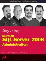
When data is added to the tree, a node will eventually become full and will need to split. Because in SQL
Server, a node equates to a page, this is called a page split, illustrated in Figure 9-3.
When a page split occurs, data is automatically moved around to keep things balanced. The first half of
the data is left on the old page, and the rest of the data is added to a new page — thus you have about a
50-50 split, and your tree remains balanced.
Figure 9-3
If you think about this splitting process a bit, you’ll realize that it adds a substantial amount of overhead
at the time of the split. Instead of inserting just one page, you are:
❑ Creating a new page
❑ Migrating rows from the existing page to the new page
❑ Adding your new row to one of the pages
❑ Adding another entry in the parent node
Ordered insert as middle record

in a Cluster Key
Since the new record needs to go in the
middle, the page must be split.
New record to be inserted,
but the page is full.
2
4
6
8
2
4
5
6
8
5
×
267
Chapter 9: SQL Server Storage and Index Structures
57012c09.qxd:WroxBeg 11/25/08 5:45 AM Page 267
But the overhead doesn’t stop there. Since we’re in a tree arrangement, you have the possibility for
something of a cascading action. When you create the new page (because of the split), you need to make
another entry in the parent node. This entry in the parent node also has the potential to cause a page
split at that level, and the process starts all over again. Indeed, this possibility extends all the way up to
and can even affect the root node.
If the root node splits, then you actually end up creating two additional pages. Because there can be only
one root node, the page that was formerly the root node is split into two pages and becomes a new inter-
mediate level of the tree. An entirely new root node is then created, and will have two entries (one to the
old root node, one to the split page).
Needless to say, page splits can have a very negative impact on system performance and are character-
ized by behavior where your process on the server seems to just pause for a few seconds (while the

pages are being split and rewritten).
We will talk about page-split prevention before we’re done with this chapter.
While page splits at the leaf level are a common fact of life, page splits at intermediate nodes happen far
less frequently. As your table grows, every layer of the index will experience page splits, but because the
intermediate nodes have only one entry for several entries on the next lower node, the number of page
splits gets less and less frequent as you move further up the tree. Still, for a split to occur above the leaf
level, there must have already been a split at the next lowest level — this means that page splits up the
tree are cumulative (and expensive performance-wise) in nature.
SQL Server has a number of different types of indexes (which we will discuss shortly), but they all make
use of this B-Tree approach in some way or another. Indeed, they are all very similar in structure, thanks
to the flexible nature of a B-Tree. Still, we shall see that there are indeed some significant differences, and
these can have an impact on the performance of our system.
For an SQL Server index, the nodes of the tree come in the form of pages, but you can actually apply this
concept of a root node, the non-leaf level, the leaf level, and the tree structure to more than just SQL
Server or even just databases.
How Data Is Accessed in SQL Server
In the broadest sense, there are only two ways in which SQL Server retrieves the data you request:
❑ Using a table scan
❑ Using an index
Which method SQL Server uses to run your particular query will depend on what indexes are available,
what columns you are asking about, what kind of joins you are doing, and the size of your tables.
Use of Table Scans
A table scan is a pretty straightforward process. When a table scan is performed, SQL Server starts at the
physical beginning of the table, looking through every row in the table. As it finds rows that match the
criteria of your query, it includes them in the result set.
268
Chapter 9: SQL Server Storage and Index Structures
57012c09.qxd:WroxBeg 11/25/08 5:45 AM Page 268
You may hear lots of bad things about table scans, and in general, they will be true. However, table scans
can actually be the fastest method of access in some instances. Typically, this is the case when retrieving

data from rather small tables. The exact size where this becomes the case will vary widely according to
the width of your table and the specific nature of the query.
See if you can spot why the use of
EXISTS in the WHERE clause of your queries has so much to offer
performance-wise when it fits the problem. When you use the
EXISTS operator, SQL Server stops as
soon as it finds one record that matches the criteria. If you had a million-record table and it found a
matching record on the third record, then use of the
EXISTS option would have saved you the reading
of 999,997 records!
NOT EXISTS works in much the same way.
Use of Indexes
When SQL Server decides to use an index, the process actually works somewhat similarly to a table scan,
but with a few shortcuts.
During the query optimization process, the optimizer takes a look at all the available indexes and
chooses the best one (this is primarily based on the information you specify in your joins and
WHERE
clause, combined with statistical information SQL Server keeps on index makeup). Once that index is
chosen, SQL Server navigates the tree structure to the point of data that matches your criteria and again
extracts only the records it needs. The difference is that since the data is sorted, the query engine knows
when it has reached the end of the current range it is looking for. It can then end the query, or move on
to the next range of data as necessary.
If you ponder the query topics we’ve studied thus far (Chapter 7 specifically), you may notice some
striking resemblances to how the
EXISTS option works. The EXISTS keyword allowed a query to quit
running the instant that it found a match. The performance gains using an index are similar or better
than
EXISTS since the process of searching for data can work in a similar fashion; that is, the server can
use the sort of the index to know when there is nothing left that’s relevant and can stop things right
there. Even better, however, is that by using an index, we don’t have to limit ourselves to Boolean situa-

tions (does the piece of data I was after exist — yes or no?). We can apply this same notion to both the
beginning and end of a range. We are able to gather ranges of data with essentially the same benefits that
using an index gives to finding data. What’s more, we can do a very fast lookup (called a
SEEK) of our
data rather than hunting through the entire table.
Don’t get the impression from my comparing what indexes do to what the
EXISTS operator does that
indexes replace the
EXISTS operator altogether (or vice versa). The two are not mutually exclusive; they
can be used together, and often are. I mention them here together only because they have the similarity of
being able to tell when their work is done, and quit before getting to the physical end of the table.
Index Types and Index Navigation
Although there are nominally two types of base index structures in SQL Server (clustered and non-clus-
tered), there are actually, internally speaking, three different types:
❑ Clustered indexes
❑ Non-clustered indexes, which comprise:
❑ Non-clustered indexes on a heap
❑ Non-clustered indexes on a clustered index
269
Chapter 9: SQL Server Storage and Index Structures
57012c09.qxd:WroxBeg 11/25/08 5:45 AM Page 269
The way the physical data is stored varies between clustered and non-clustered indexes. The way SQL
Server traverses the B-Tree to get to the end data varies between all three index types.
All SQL Server indexes have leaf level and non-leaf level pages. As we mentioned when we discussed B-
Trees, the leaf level is the level that holds the “key” to identifying the record, and the non-leaf level
pages are guides to the leaf level.
The indexes are built over either a clustered table (if the table has a clustered index) or what is called a
heap (what’s used for a table without a clustered index).
Clustered Tables
A clustered table is any table that has a clustered index on it. Clustered indexes are discussed in detail

shortly, but what they mean to the table is that the data is physically stored in a designated order. Indi-
vidual rows are uniquely identified through the use of the cluster key — the columns that define the clus-
tered index.
This should bring to mind the question, “What if the clustered index is not unique?” That is, how can a
clustered index be used to uniquely identify a row if the index is not a unique index? The answer lies
under the covers: SQL Server forces any clustered indexes to be unique — even if you don’t define them
that way. Fortunately, it does this in a way that doesn’t change how you use the index. You can still
insert duplicate rows if you wish, but SQL Server will add a suffix to the key internally to ensure that
the row has a unique identifier.
Heaps
A heap is any table that does not have a clustered index on it. In this case, a unique identifier, or row ID
(RID), is created based on a combination of the extent, pages, and row offset (places from the top of the
page) for that row. A RID is only necessary if there is no cluster key available (no clustered index).
Clustered Indexes
A clustered index is unique for any given table — you can only have one per table. You don’t have to have
a clustered index, but you’ll find it to be one of the most commonly chosen types for a variety of reasons
that will become apparent as we look at our index types.
What makes a clustered index special is that the leaf level of a clustered index is the actual data — that
is, the data is re-sorted to be stored in the same physical order of the index sort criteria state. This means
that once you get to the leaf level of the index, you’re done; you’re at the data. Any new record is inserted
according to its correct physical order in the clustered index. How new pages are created changes depending
on where the record needs to be inserted.
In the case of a new record that needs to be inserted into the middle of the index structure, a normal
page split occurs. The last half of the records from the old page are moved to the new page, and the new
record is inserted into the new or old page as appropriate.
In the case of a new record that is logically at the end of the index structure, a new page is created, but
only the new record is added to the new page, as shown in Figure 9-4.
270
Chapter 9: SQL Server Storage and Index Structures
57012c09.qxd:WroxBeg 11/25/08 5:45 AM Page 270

Figure 9-4
Navigating the Tree
As I’ve indicated previously, even the indexes in SQL Server are stored in a B-Tree. Theoretically, a
B-Tree always has half of the remaining information in each possible direction as the tree branches. Let’s
take a look at a visualization of what a B-Tree looks like for a clustered index (Figure 9-5).
Figure 9-5
Root
Looking for Records
158 through 400
Non-Leaf
Level
1
157
•••
•••
Bob
Sam
•••
•••
George
53
54
103
Fred
Sally
•••
•••
Steve
1
2

52
Bruce
Sue
•••
•••
•••
104
105
156
Bill
•••
•••
Margot
Tom
270
271
400
401
Tom
Ashley
•••
•••
Ralph
157
158
269
Mike
Nancy
411
412

1
53
104
157
270
410
Leaf Level
is Data Page
Ordered insert as last record
in a Cluster Key
New record to be inserted
but the page is full. Since it
is last, it is added to an
entirely new page without
disturbing the existing data.
1
2
3
4
5
5
×
271
Chapter 9: SQL Server Storage and Index Structures
57012c09.qxd:WroxBeg 11/25/08 5:45 AM Page 271
As you can see, it looks essentially identical to the more generic B-Trees we discussed earlier in the chap-
ter. In this case, we’re doing a range search (something clustered indexes are particularly good at) for
numbers 158–400. All we have to do is navigate to the first record and include all remaining records on
that page. We know we need the rest of that page because the information from the node one level up
lets us know that we’ll also need data from a few other pages. Because this is an ordered list, we can be

sure it’s continuous — that means if the next page has records that should be included, then the rest of
this page must be included. We can just start spewing out data from those pages without having to do
any verification.
We start off by navigating to the root node. SQL Server is able to locate the root node based on an entry
that you can see in the system metadata view called
sys.indexes.
By looking through the page that serves as the root node, we can figure out what the next page we need
to examine is (the second page on the second level as we have it drawn here). We then continue the
process. With each step we take down the tree, we are getting to smaller and smaller subsets of data.
Eventually, we will get to the leaf level of the index. In the case of our clustered index, getting to the leaf
level of the index means that we are also at our desired row(s) and our desired data.
Non-Clustered Indexes on a Heap
Non-clustered indexes on a heap work very similarly to clustered indexes in most ways. They do, however,
have a few notable differences:
The leaf level is not the data — instead, it is the level at which you are able to obtain a pointer to that
data. This pointer comes in the form of a row identifier or RID, which, as we described earlier in the
chapter, is made up of the extent, page, and row offset for the particular row being pointed to by the
index. Even though the leaf level is not the actual data (instead, it has the RID), we only have one more
step than with a clustered index. Because the RID has the full information on the location of the row, we
can go directly to the data.
Don’t, however, misunderstand this “one more step” to mean that there’s only a small amount of over-
head difference and that non-clustered indexes on a heap will run close to as fast as a clustered index.
With a clustered index, the data is physically in the order of the index. That means, for a range of data,
when you find the row that has the beginning of your data on it, there’s a good chance that the other
rows are on that page with it (that is, you’re already physically almost to the next record since they are
stored together). With a heap, the data is not linked together in any way other than through the index.
From a physical standpoint, there is absolutely no sorting of any kind. This means that from a physical
read standpoint, your system may have to retrieve records from all over the file. Indeed, it’s quite possi-
ble (possibly even probable) that you will wind up fetching data from the same page several separate
times. SQL Server has no way of knowing it will have to come back to that physical location because

I can’t stress enough the importance of this distinction: With a clustered index, when
you’ve fully navigated the index, you’ve fully navigated to your data. How much of
a performance difference this can make will really show its head as we look at non-
clustered indexes — particularly when the non-clustered index is built over a clustered
index.
272
Chapter 9: SQL Server Storage and Index Structures
57012c09.qxd:WroxBeg 11/25/08 5:45 AM Page 272
there was no link between the data. With the clustered index, it knows that’s the physical sort, and can
therefore grab it all in just one visit to the page.
Just to be fair to the non-clustered index on a heap here vs. the clustered index, the odds are extremely
high that any page that was already read once will still be in the memory cache and, as such, will be
retrieved extremely quickly. Still, it does add some additional logical operations to retrieve the data.
Figure 9-6 shows the same search we performed on the clustered index, only with a non-clustered index
on a heap this time.
Through most of the index navigation, things work exactly as they did before. We start out at the same
root node, and we traverse the tree dealing with more and more focused pages until we get to the leaf
level of our index. This is where we run into the difference. With a clustered index, we could have
stopped right here, but with a non-clustered index, we have more work to do. If the non-clustered index
is on a heap, then we have just one more level to go. We take the Row ID from the leaf level page and
navigate to it. It is not until this point that we are at our actual data.
Figure 9-6
Non-Clustered Indexes on a Clustered Table
With non-clustered indexes on a clustered table, the similarities continue — but so do the differences. Just
as with non-clustered indexes on a heap, the non-leaf level of the index looks pretty much as it did for a
clustered index. The difference does not come until we get to the leaf level.
Root
Looking for Records
158 through 400
Non-Leaf

Level
1
157
•••
•••
100403
236201
•••
•••
241905
53
54
103
476405
236205
•••
•••
111903
1
2
52
334205
141604
•••
•••
020001
104
105
156
220703

236204
•••
127504
126003
270
271
400
401
141602
220702
•••
•••
220701
157
158
269
151501
102404
411
412
Ralph
Ashley
Bill
•••
•••
220701
220702
220703
220704
220701

Bob
Sue
Tony
•••
George
241901
241902
241903
241904
241905
Nick
Don
Kate
Tony
Francis
236201
236202
236203
236204
236205
1
53
104
157
270
410
Leaf Level
Data Pages
273
Chapter 9: SQL Server Storage and Index Structures

57012c09.qxd:WroxBeg 11/25/08 5:45 AM Page 273
At the leaf level, we have a rather sharp difference from what we’ve seen with the other two index struc-
tures: We have yet another index to look over. With clustered indexes, when we got to the leaf level, we
found the actual data. With non-clustered indexes on a heap, we didn’t find the actual data, but did find
an identifier that let us go right to the data (we were just one step away). With non-clustered indexes on
a clustered table, we find the cluster key. That is, we find enough information to go and make use of the
clustered index.
We end up with something that looks like Figure 9-7.
What we end up with is two entirely different kinds of lookups.
In the example from our diagram, we start off with a ranged search. We do one single lookup in our
index and are able to look through the non-clustered index to find a continuous range of data that meets
our criterion (
LIKE ‘T%’). This kind of lookup, where we can go right to a particular spot in the index,
is called a seek.
The second kind of lookup then starts — the lookup using the clustered index. This second lookup is
very fast; the problem lies in the fact that it must happen multiple times. You see, SQL Server retrieved a
list from the first index lookup (a list of all the names that start with “T”), but that list doesn’t logically
match up with the cluster key in any continuous fashion. Each record needs to be looked up individually,
as shown in Figure 9-8.
Needless to say, this multiple-lookup situation introduces more overhead than if we had just been able to
use the clustered index from the beginning. The first index search — the one through our non-clustered
index — requires very few logical reads.
For example, if I have a table with 1,000 bytes per row and I do a lookup similar to the one in our draw-
ing (say, something that would return five or six rows); it would only take something to the order of
8–10 logical reads to get the information from the non-clustered index. However, that only gets me as far
as being ready to look up the rows in the clustered index. Those lookups would cost approximately 3–4
logical reads each, or 15–24 additional reads. That probably doesn’t seem like that big a deal at first, but
look at it this way:
Logical reads went from 3 minimum to 24 maximum — that’s an 800 percent increase in the amount of
work that had to be done.

Now expand this thought out to something where the range of values from the non-clustered index wasn’t
just five or six rows, but five or six thousand, or five or six hundred thousand rows — that’s going to be a
huge impact.
Don’t let the extra overhead vs. a clustered index scare you — the point isn’t meant to scare you away
from using indexes, but rather to point out that a non-clustered index is generally not going to be as
efficient as a clustered index from a read perspective (it can, in some instances, actually be a better
choice at insertion time). An index of any kind is usually (there are exceptions) the fastest way to do a
lookup. We’ll explain what index to use and why later in the chapter.
274
Chapter 9: SQL Server Storage and Index Structures
57012c09.qxd:WroxBeg 11/25/08 5:45 AM Page 274
Figure 9-7
Root
Non-Leaf
Level
115
1
56
74
52
Select EmployeeID
who is FName like “T%”
To Clustered
Index Point
52
157
99
Steve
Tom
Zach

115
270
23
361
211
Allison
Bill
Charlie
Diane
Ernest
Allison
Fred
Mike
Ralph
Steve
52
105
102
Steve
Sue
•••
•••
Tim
270
104
171
Bill
Bruce
•••
•••

Frank
Bill
Russ
•••
•••
Tom
270
276
401
Tom
Ashley
•••
Tony
•••
Ralph
157
158
209
269
Bob
Sam
•••
•••
Tim
George
53
54
102
103
Fred

Sally
•••
•••
Steve
1
2
52
115
27
367
Allison
Amy
•••
•••
Barbara
157
209
Tom
Tony
•••
•••
Yolanda
Leaf Level
1
157
•••
•••
157
270
410

1
53
104
275
Chapter 9: SQL Server Storage and Index Structures
57012c09.qxd:WroxBeg 11/25/08 5:45 AM Page 275
Figure 9-8
Creating, Altering, and Dropping Indexes
These work much as they do on other objects such as tables. Let’s take a look at each, starting with the
CREATE.
Indexes can be created in two ways:
❑ Through an explicit
CREATE INDEX command
❑ As an implied object when a constraint is created
Each of these has its own quirks about what it can and can’t do, so let’s look at each of them
individually.
Tim
Fred
Mike
Ralph
Tony
102
1
56
74
209
Tony
Tom
Zach
209

157
99
Tim
Bill
Charlie
Diane
Ernest
102
270
23
361
211
Tom
Tony
•••
•••
Yolanda
157
209
Tony
Sue
•••
•••
Tim
105
102
Bill
Bruce
•••
•••

Frank
270
104
171
Tim
Amy
•••
•••
Barbara
102
27
367
Tim
Fred
Mike
Ralph
Steve
102
1
56
74
52
Steve
Tom
Zach
52
157
99
Tim
Bill

Charlie
Diane
Ernest
102
270
23
361
211
Tom
Tony
•••
•••
Yolanda
157
209
Steve
Sue
•••
•••
Tim
52
105
102
Bill
Bruce
•••
•••
Frank
270
104

171
Tim
Amy
•••
•••
Barbara
102
27
367
Tom
Fred
Mike
Ralph
Steve
157
1
56
74
52
Tim
Tom
Tony
Clustered Seek: 102
Clustered Seek: 209
List from
Non-Clustered Index:
Clustered Seek: 157
102
157
209

Steve
Tom
Zach
52
157
99
Tom
Bill
Charlie
Diane
Ernest
157
270
23
361
211
Tom
Tony
•••
•••
Yolanda
157
209
Steve
Sue
•••
•••
Tim
52
105

102
Bill
Bruce
•••
•••
Frank
270
104
171
Tom
Amy
•••
•••
Barbara
157
27
367
276
Chapter 9: SQL Server Storage and Index Structures
57012c09.qxd:WroxBeg 11/25/08 5:45 AM Page 276
The CREATE INDEX Statement
The CREATE INDEX statement does exactly what it sounds like — it creates an index on the specified
table or view based on the stated columns.
The syntax to create an index is somewhat drawn out and introduces several items that we haven’t
really talked about up to this point:
CREATE [UNIQUE] [CLUSTERED|NONCLUSTERED]
INDEX <index name> ON <table or view name>(<column name> [ASC|DESC] [, n])
INCLUDE (<column name> [, n])
[WITH
[PAD_INDEX = { ON | OFF }]

[[,] FILLFACTOR = <fillfactor>]
[[,] IGNORE_DUP_KEY = { ON | OFF }]
[[,] DROP_EXISTING = { ON | OFF }]
[[,] STATISTICS_NORECOMPUTE = { ON | OFF }]
[[,] SORT_IN_TEMPDB = { ON | OFF }]
[[,] ONLINE = { ON | OFF }
[[,] ALLOW_ROW_LOCKS = { ON | OFF }
[[,] ALLOW_PAGE_LOCKS = { ON | OFF }
[[,] MAXDOP = <maximum degree of parallelism>
]
[ON {<filegroup> | <partition scheme name> | DEFAULT }]
There is legacy syntax available for many of these options, and so you may see that syntax put into use
to support prior versions of SQL Server. That syntax is, however, considered deprecated and will be
removed at some point. I highly recommend that you stay with the newer syntax where possible.
Loosely speaking, this statement follows the same
CREATE <object type> <object name> syntax
that we’ve seen plenty of already (and will see even more of). The primary hitch in things is that we
have a few intervening parameters that we haven’t seen elsewhere.
Just as we’ll see with views in our next chapter, we do have to add an extra clause onto our
CREATE
statement to deal with the fact that an index isn’t really a stand-alone kind of object. It has to go together
with a table or view, and we need to state the table that our column(s) are
ON.
After the
ON <table or view name>(<column name>) clause, everything is optional. You can mix
and match these options. Many of them are seldom used, but some (such as
FILLFACTOR) can have a
significant impact on system performance and behavior, so let’s look at them one by one.
ASC/DESC
These two allow you to choose between an ascending and a descending sort order for your index. The

default is
ASC, which is, as you might guess, ascending order.
There is a similar but sufficiently different syntax for creating XML indexes. That
will be handled separately at the end of this section.
277
Chapter 9: SQL Server Storage and Index Structures
57012c09.qxd:WroxBeg 11/25/08 5:45 AM Page 277
A question that might come to mind is why ascending vs. descending matters — SQL Server can just
look at an index backwards if it needs the reverse sort order. Life is not, however, always quite so simple.
Looking at the index in reverse order works just fine if you’re dealing with only one column, or if your
sort is always the same for all columns, but what if you needed to mix sort orders within an index? That
is, what if you need one column to be sorted ascending, but the other descending? Since the indexed
columns are stored together, reversing the way you look at the index for one column would also reverse
the order for the additional columns. If you explicitly state that one column is ascending and the other is
descending, then you invert the second column right within the physical data — there is suddenly no
reason to change the way that you access your data.
As a quick example, imagine a reporting scenario where you want to order your employee list by the
hire date, beginning with the most recent (a descending order), but you also want to order by their last
name (an ascending order). Before indexes were available, SQL Server would have to do two opera-
tions — one for the first column and one for the second. Having control over the physical sort order of
our data provides flexibility in the way we can combine columns.
INCLUDE
This one is supported with SQL Server 2005 and later. Its purpose is to provide better support for what
are called covered queries.
When you
INCLUDE columns as opposed to placing them in the ON list, SQL Server only adds them at the
leaf level of the index. Because each row at the leaf level of an index corresponds to a data row, what
you’re doing is essentially including more of the raw data in the leaf level of your index. If you think
about this, you can probably make the guess that
INCLUDE really applies only to non-clustered indexes

(clustered indexes already are the data at the leaf level, so there would be no point).
Why does this matter? Well, as we’ll discuss further as the book goes on, SQL Server stops working as
soon as it has what it actually needs. So if while traversing the index it can find all the data that it needs
without continuing to the actual data row, then it won’t bother going to the data row (what would be the
point?). By including a particular column in the index, you may “cover” a query that utilizes that particu-
lar index at the leaf level and save the I/O associated with using that index pointer to go to the data page.
Careful not to abuse this one! When you include columns, you are enlarging the size of the leaf level of
your index pages. That means fewer rows will fit per page, and therefore, more I/O may be required to
see the same number of rows. The result may be that your effort to speed up one query may slow down
others. To quote an old film from the eighties, “Balance, Danielson — balance!” Think about the effects
on all parts of your system, not just the particular query you’re working on that moment.
WITH
WITH is an easy one; it just tells SQL Server that you will indeed be supplying one or more of the options
that follow.
PAD_INDEX
In the syntax list, this one comes first — but that will seem odd when you understand what PAD_INDEX
does. In short, it determines just how full the non-leaf level pages of your index are going to be (as a per-
centage) when the index is first created. You don’t state a percentage on
PAD_INDEX because it will use
whatever percentage you specify in the
FILLFACTOR option that follows. Setting PAD_INDEX = ON
would be meaningless without a FILLFACTOR (which is why it seems odd that it comes first).
278
Chapter 9: SQL Server Storage and Index Structures
57012c09.qxd:WroxBeg 11/25/08 5:45 AM Page 278
FILLFACTOR
When SQL Server first creates an index, the pages are, by default, filled as full as they can be, minus two
records. You can set the
FILLFACTOR to be any value between 1 and 100. This number will determine
how full your pages are as a percentage, once index construction is completed. Keep in mind, however,

that as your pages split, your data will still be distributed 50-50 between the two pages — you cannot
control the fill percentage on an ongoing basis other than regularly rebuilding the indexes (something
you should do).
We use a
FILLFACTOR when we need to adjust the page densities. Think about things this way:
❑ If it’s an OLTP system, you want the
FILLFACTOR to be low.
❑ If it’s an OLAP or other very stable (in terms of changes — very few additions and deletions)
system, you want the
FILLFACTOR to be as high as possible.
❑ If you have something that has a medium transaction rate and a lot of report-type queries
against it, then you probably want something in the middle (not too low, not too high).
If you don’t provide a value, then SQL Server will fill your pages to two rows short of full, with a mini-
mum of one row per page (for example, if your row is 8,000 characters wide, you can fit only one row
per page, so leaving things two rows short wouldn’t work).
IGNORE_DUP_KEY
The IGNORE_DUP_KEY option is a way of doing little more than circumventing the system. In short, it
causes a unique constraint to have a slightly different action from that which it would otherwise have.
Normally, a unique constraint, or unique index, does not allow any duplicates of any kind — if a trans-
action tried to create a duplicate based on a column that is defined as unique, then that transaction would
be rolled back and rejected. After you set the
IGNORE_DUP_KEY option, however, you’ll get mixed behavior.
You will still receive an error message, but the error will only be of a warning level. The record is still not
inserted.
This last line —
the record is still not inserted — is a critical concept from an IGNORE_DUP_KEY
standpoint. A rollback isn’t issued for the transaction (the error is a warning error rather than a critical
error), but the duplicate row will have been rejected.
Why would you do this? Well, it’s a way of storing unique values without disturbing a transaction that
tries to insert a duplicate. For whatever process is inserting the would-be duplicate, it may not matter at

all that it’s a duplicate row (no logical error from it). Instead, that process may have an attitude that’s
more along the lines of, “Well, as long as I know there’s one row like that in there, I’m happy — I don’t
care whether it’s the specific row that I tried to insert or not.”
DROP_EXISTING
If you specify the DROP_EXISTING option, any existing index with the name in question will be dropped
prior to construction of the new index. This option is much more efficient than simply dropping and
re-creating an existing index when you use it with a clustered index. If you rebuild an exact match of the
existing index, SQL Server knows that it need not touch the non-clustered indexes, while an explicit
drop and create would involve rebuilding all non-clustered indexes twice in order to accommodate
279
Chapter 9: SQL Server Storage and Index Structures
57012c09.qxd:WroxBeg 11/25/08 5:45 AM Page 279