Table 5.6 lists several TPA issues, indicates whether or not they are an advan-
tage or disadvantage (if applicable), and points to where in the book the
reader may find additional information. Some analysis has been performed
on the TPA set of techniques (see the performance section below), but more
research and experimentation is required before they can be used with
confidence.
The indication that an issue in Table 5.6 can be a positive or negative
(+/−) influence on the technique or on its effectiveness further indicates that
the issue may be a disadvantage in general (e.g., cost is higher than non-
fault-tolerant software) but an advantage in relation to another technique. In
Data Diverse Software Fault Tolerance Techniques !
Table 5.6
Two-Pass Adjudi cator Issue Summary
Issue
Advantage (+)/
Disadvantage (−) Where Discussed
Provides protection against errors in tr anslating
requirements and functionality into code (true for
software fault tolerance techniq ues in general)
+ Chapter 1
Does not provi de explicit pro tection against errors
in specifying requirements (true for software fault
tolerance techniques in general)
− Chapter 1
General backward and forward recovery
advantages
+ Sections 1.4.1, 1.4.2
General backward and forward recovery
disadvantages
− Sections 1.4.1, 1.4.2
General design and data diversi ty advantages + Sections 2.2, 2.3

General design and data diversi ty disadvantages − Sections 2.2, 2.3
DRA +/− Sections 2.3.12.3.3
Similar errors or common residua l design errors − Section 3.1.1
Coincident and correlated failures − Section 3.1.1
CCP − Section 3.1.2
Space and time redundancy +/− Section 3.1.4
Design conside rations + Section 3.3.1
Dependable system development model + Section 3.3.2
Dependability studies +/− Section 4.1.3. 3
Voters and discussions related to specific types of
voters
+/− Section 7.1
these cases, the reader is referred to the noted section for discussion of the
issue.
5.3.4.1 Architecture
We mentioned in Sections 1.3.1.2 and 2.5 that structuring is required if we
are to handle system complexity, especially when fault tolerance is involved
[1315]. This includes defining the organization of software modules onto
the hardware elements on which they run. The TPA is typically multi-
processor, with components residing on n hardware units and the executive
residing on one of the processors. Communications between the software
components is done through remote function calls or method invocations.
5.3.4.2 Performance
There have been numerous investigations into the performance of software
fault tolerance techniques in general (discussed in Chapters 2 and 3) and the
dependability of specific techniques themselves. Table 4.2 (in Section 4.1.3.3)
provides a list of references for these dependability investigations. This list,
although not exhaustive, provides a good sampling of the types of analyses
that have been performed and substantial background for analyzing software
fault tolerance dependability. The reader is encouraged to examine the refer-

ences for details on assumptions made by the researchers, experiment design,
and results interpretation.
The fault tolerance of a system employing data diversity depends upon
the ability of the DRA to produce data points that lie outside of a failure
region, given an initial data point that lies within a failure region. The pro-
gram executes correctly on re-expressed data points only if they lie outside a
failure region. If the failure region has a small cross section in some dimen-
sions, then re-expression should have a high probability of translating the
data point out of the failure region.
Pullum [7] provides a formulation for determination of the prob-
abilities that each TPA solution has of producing a correct adjudged result.
Expected execution times and additional performance details are provided by
the author in [7].
5.4 Summary
This chapter presented the two original data diverse techniques, NCP and
RtB, and a spin-off, TPA. The data diverse techniques are offered as a
complement to the battery of design diverse techniques and are not meant to
232 Software Fault Tolerance Techniques and Implementation
replace them. RtB are similar in structure to the RcB, as NCP is similar
to NVP. The primary difference in operation is the attribute diversified.
The TPA technique uses both data and design diversity to avoid and handle
MCR. For each technique, its operation, an example, and issues were pre-
sented. Pointers to the original source and to extended examinations of the
techniques were provided for the readers additional study, if desired.
The following chapter examines several other techniquesthose not
easily categorized as design or data diverse and those different enough to war-
rant belonging to this separate grouping. These techniques are discussed in
much the same manner as were those in this chapter and the techniques
in Chapter 4.
References

[1] Ammann, P. E., Data Diversity: An Approach to Software Fault Tolerance, Proceed-
ings of FTCS-17, Pittsburgh, PA, 1987, pp. 122126.
[2] Ammann, P. E., Data Diversity: An Approach to Software Fault Tolerance, Ph.D.
dissertation, University of Virginia, 1988.
[3] Ammann, P. E., and J. C. Knight, Data Diversity: An Approach to Software Fault
Tolerance, IEEE Transactions on Computers, Vol. 37, No. 4, 1988, pp. 418425.
[4] Gray, J., Why Do Computers Stop and What Can Be Done About It? Tandem, Techni-
cal Report 85.7, 1985.
[5] Martin, D. J., Dissimilar Software in High Integrity Applications in Flight Control,
Software for Avionics, AGARD Conference Proceedings, 1982, pp. 36-136-13.
[6] Morris, M. A., An Approach to the Design of Fault Tolerant Software, M.Sc. thesis,
Cranfield Institute of Technology, 1981.
[7] Pullum, L. L., Fault Tolerant Software Decision-Making Under the Occurrence of
Multiple Correct Results, Doctoral dissertation, Southeastern Institute of Technol-
ogy, 1992.
[8] Pullum, L. L., A New Adjudicator for Fault Tolerant Software Applications Correctly
Resulting in Multiple Solutions, Quality Research Associates, Technical Report
QRA-TR-92-01, 1992.
[9] Pullum, L. L., A New Adjudicator for Fault Tolerant Software Applications Correctly
Resulting in Multiple Solutions, Proceedings: 12th Digital Avionics Systems Conference,
Fort Worth, TX, 1993.
[10] Ammann, P. E., D. L. Lukes, and J. C. Knight, Applying Data Diversity to Differential
Equation Solvers. in Software Fault Tolerance Using Data Diversity, University of
Virginia Technical Report, Report No. UVA/528344/CS92/101, for NASA Langley
Research Center, Grant No. NAG-1-1123, 1991.
Data Diverse Software Fault Tolerance Techniques !!
[11] Ammann, P. E., and J. C. Knight, Data Re-expression Techniques for Fault Tolerant
Systems, Technical Report, Report No. TR90-32, Department of Computer Science,
University of Virginia, 1990.
[12] Ammann, P. E., Data Redundancy for the Detection and Tolerance of Software

Faults, Proceedings: Interface 90, East Lansing, MI, 1990.
[13] Anderson, T., and P. A. Lee, Software Fault Tolerance, in Fault Tolerance: Principles
and Practice, Englewood Cliffs, NJ: Prentice-Hall, 1981, pp. 249291.
[14] Randell, B., Fault Tolerance and System Structuring, Proceedings 4th Jerusalem
Conference on Information Technology, Jerusalem, 1984, pp. 182191.
[15] Neumann, P. G., On Hierarchical Design of Computer Systems for Critical Applica-
tions, IEEE Transactions on Software Engineering, Vol. 12, No. 9, 1986, pp. 905920.
[16] McAllister, D. F., and M. A. Vouk, Fault-Tolerant Software Reliability Engineering,
in M. R. Lyu (ed.), Handbook of Software Reliability Engineering, New York: IEEE
Computer Society Press, 1996, pp. 567614.
[17] Duncan, R. V., Jr., and L. L. Pullum, Object-Oriented Executives and Components
for Fault Tolerance, IEEE Aerospace Conference, Big Sky, MT, 2001.
234 Software Fault Tolerance Techniques and Implementation
6
Other Software Fault Tolerance
Techniques
New techniques are often proposed to overcome the limitations associated
with previous techniques, to provide fault tolerance for specific problem
domains, or to apply new technologies to the needs of software fault toler-
ance, while attempting to maintain the strengths of the foundational tech-
niques. This chapter covers some of these other software fault tolerance
techniques, those that do not necessarily fit nicely into either the design or
data diverse categoriesvariants of the N-version programming (NVP) tech-
nique, resourceful systems, the data-driven dependability assurance scheme,
self-configuring optimal programming (SCOP), and other software fault tol-
erance techniques.
6.1 N-Version Programming Variants
Numerous variations on the basic NVP technique have been proposed.
These NVP variants range from simple use of a decision mechanism (DM)
other than the basic majority voter (see Section 7.1 for some alternatives)

to combinations with other techniques (see, for example, the consensus
recovery block (CRB) and acceptance voting (AV) techniques described in
Sections 4.5 and 4.6, respectively) to those that appear to be an entirely new
technique (for example, the two-pass adjudicators (TPA), Section 5.3). As
!#
stated above, many of these techniques arise from a real or perceived defi-
ciency in the original technique.
In this section, we will examine one such NVP variant, the NVP-
TB-AT (N-version programming with a tie-breaker and an acceptance test
(AT)) technique, developed by Ann Tai and colleagues [13]. The technique
was developed to illustrate performability modeling and making design
modifications to enhance performability. Tai defines performability as a uni-
fication of performance and dependability, that is, a systems ability to per-
form (serve its users) in the presence of fault-caused errors and failures [1].
See Section 4.7.1 for an overview of the performability investigation for
the NVP and recovery block (RcB) techniques. (Also see [13] for a more
detailed discussion.)
The NVP-TB-AT technique was developed by combining the per-
formability advantages of two modified NVP techniques, the NVP-TB
(NVP with a tie-breaker) and NVP-AT (NVP with an AT). Hence,
NVP-TB-AT incorporates both a tie-breaker and an AT. When the prob-
ability of related faults is low, the efficient synchronization provided by the
tie-breaker mechanism compensates for the performance reduction caused
by the AT. The AT is applied only when the second DM reaches a consensus
decision. When the probability of related faults is high, the additional error
detection provided by the AT reduces the likelihood (due to the high execu-
tion rate of NVP-TB) of an undetected error [3].
NVP-TB-AT is a design diverse, forward recovery (see Section 1.4.2)
technique. The technique uses multiple variants of a program, which run
concurrently on different computers. The results of the first two variants to

finish their execution are gathered and compared. If the results match, they
are output as the correct result. If the results do not match, the technique
waits for the third variant to finish. When it does, a majority voter-type DM
is used on all three results. If a majority is found, the matching result must
pass the AT before being output as the correct result.
NVP-TB-AT operation is described in Section 6.1.1 An example is
provided in Section 6.1.2. The techniques performance was discussed in
Section 4.7.1.
6.1.1 N-Version Programming with Tie-Breaker and Acceptance
Test Operation
The NVP-TB-AT technique consists of an executive, n variants (three vari-
ants are used in this discussion) of the program or function, and several
DMs: a comparator, a majority voter, and an AT. The executive orchestrates
the NVP-TB-AT technique operation, which has the general syntax:
236 Software Fault Tolerance Techniques and Implementation
TEAMFLY























































Team-Fly
®

run Variant 1, Variant 2, Variant 3
if (Comparator (Fastest Result 1,
Fastest Result 2))
return Result
else Wait (Last Result)
if (Voter (Fastest Result 1,
Fastest Result 2,
Last Result))
if (Acceptance Test (Result))
return Result
else error
The NVP-TB-AT syntax above states that the technique executes the
three variants concurrently. The results of the two fastest running of these
executions are provided to the comparator, which compares the results to
determine if they are equal. If they are, then the result is returned as the pre-
sumed correct result. If they are not equal, then the technique waits for the
slowest variant to produce a result. Given results from all variants, the major-
ity voter DM determines if a majority of the results are equal. If a majority

is found, then that result is tested by an AT. If the result is acceptable, it
is output as the presumed correct result. Otherwise, an error exception is
raised. Figure 6.1 illustrates the structure and operation of the NVP-TB-AT
technique.
Both fault-free and failure scenarios for NVP-TB-AT are described
below. The following abbreviations are used:
AT Acceptance test;
V
i
Variant i;
n The number of versions (n = 3);
NVP-TB-AT N-version programming with tie-breaker and
acceptance test;
R
i
Result occurring in the ith order; that is, R
1
is the
fastest, R
3
is the slowest;
R Result of NVP-TB-AT.
6.1.1.1 Failure-Free Operation
This scenario describes the operation of NVP-TB-AT when no failure or
exception occurs.
Other Software Fault Tolerance Techniques 237
•
Upon entry to the NVP-TB-AT, the executive performs the follow-
ing: formats calls to the three variants and through those calls dis-
tributes the input(s) to the variants.

•
Each variant, 8
E
, executes. No failures occur during their execution.
•
The results of the two fastest variant executions (4
1
and 4
2
) are gath-
ered by the executive and submitted to the comparator.
238 Software Fault Tolerance Techniques and Implementation
NVP-TB-AT entry NVP-TB-AT
No consensus
Distribute
inputs
Version 2
Comparator
NVP-TB-AT exit
Failure
exception
Gather results (of two fastest
versions, then slowest)
Version 3
Version 1
Results from two fastest versions
Result from
slowest version
Exception
raised

Majority
output
selected
Voter
Consensus
output
selected
No majority
AT
Result
accepted
Result not
accepted
Success:
Consensus
output
Success:
Accepted
output
Figu re 6.1 N-version progra mming wit h tie-bre aker and acceptance te st structure and
oper ation.
•
R
1
= R
2
, so the comparator sets R = R
1
= R
2

, as the correct result.
•
Control returns to the executive.
•
The executive passes the correct result outside the NVP-TB-AT, and
the NVP-TB-AT module is exited.
6.1.1.2 Partial Failure ScenarioResults Fail Comparator, Pass Voter, Pass
Acceptance Test
This scenario describes the operation of NVP-TB-AT when the compara-
tor cannot determine a correct result, but the result from the slowest variant
forms a majority with one of the other results and that majority result passes
the AT. Differences between this scenario and the failure-free scenario are in
gray type.
• Upon entry to the NVP-TB-AT, the executive performs the follow-
ing: formats calls to the three variants and through those calls dis-
tributes the input(s) to the variants.
• Each variant, V
i
, executes. No failures occur during their execution.
• The results of the two fastest variant executions (R
1
and R
2
) are gath-
ered by the executive and submitted to the comparator.
•
R
1
≠ R
2

, so the comparator cannot determine a correct result.
•
Control returns to the executive, which waits for the result from the
slowest executing variant.
•
The slowest executing variant completes execution.
•
The result from the slowest variant, R
3
, is gathered by the executive,
and along with R
1
and R
2
, is submitted to the majority voter.
•
R
3
= R
2
, so the majority voter sets R = R
2
= R
3
as the correct result.
•
Control returns to the executive.
•
The executive submits the majority result, R, to the AT.
•

The AT determines that R is an acceptable result.
•
Control returns to the executive.
•
The executive passes the correct result outside the NVP-TB-AT, and
the NVP-TB-AT module is exited.
Other Software Fault Tolerance Techniques 239
6.1.1.3 Failure ScenarioResults Fail Comparator, Pass Voter,
Fail Acceptance Test
This scenario describes the operation of NVP-TB-AT when the compara-
tor cannot determine a correct result, but the result from the slowest variant
forms a majority with one of the other results; however that majority result
does not pass the AT. Differences between this scenario and the failure-free
scenario are in gray type.
•
Upon entry to the NVP-TB-AT, the executive performs the follow-
ing: formats calls to the three variants and through those calls dis-
tributes the input(s) to the variants.
•
Each variant, 8
E
, executes. No failures occur during their execution.
•
The results of the two fastest variant executions (4
1
and 4
2
) are gath-
ered by the executive and submitted to the comparator.
•

4
1
≠ 4
2
, so the comparator cannot determine a correct result.
• Control returns to the executive, which waits for the result from the
slowest executing variant.
• The slowest executing variant completes execution.
•
The result from the slowest variant, 4
3
, is gathered by the executive,
and along with 4
1
and 4
2
, is submitted to the majority voter.
•
4
3
= 4
2
, so the majority voter sets 4 = 4
2
= 4
3
as the correct result.
•
Control returns to the executive.
•

The executive submits the majority result, 4, to the AT.
•
4 fails the AT.
•
Control returns to the executive.
•
The executive raises an exception and the NVP-TB-AT module is
exited.
6.1.1.4 Failure ScenarioResults Fail Comparator, Fail Voter
This scenario describes the operation of NVP-TB-AT when the comparator
cannot determine a correct result and the result from the slowest variant does
not form a majority with one of the other results. Differences between this
scenario and the failure-free scenario are in gray type.
240 Software Fault Tolerance Techniques and Implementation
•
Upon entry to the NVP-TB-AT, the executive performs the follow-
ing: formats calls to the three variants and through those calls dis-
tributes the input(s) to the variants.
•
Each variant, V
i
, executes. No failures occur during their execution.
•
The results of the two fastest variant executions (R
1
and R
2
) are gath-
ered by the executive and submitted to the comparator.
•

R
1
≠ R
2
, so the comparator cannot determine a correct result.
•
Control returns to the executive, which waits for the result from the
slowest executing variant.
•
The slowest executing variant completes execution.
•
The result from the slowest variant, R
3
, is gathered by the executive,
and along with R
1
and R
2
, is submitted to the majority voter.
•
R
1
≠ R
2
≠ R
3
, so the majority voter cannot determine a correct result.
• Control returns to the executive.
• The executive raises an exception and the NVP-TB-AT module is
exited.

An additional scenario will be mentioned, but not examined in detail, as
done above. That is, it is also possible that one of the variants fails to pro-
duce any result because of an endless loop (or possible hardware malfunc-
tion). This failure to produce a result event is handled by NVP-TB-AT
with a time-out and the return of a null result.
6.1.1.5 Architecture
We mentioned in Sections 1.3.1.2 and 2.5 that structuring is required if we
are to handle system complexity, especially when fault tolerance is involved
[46]. This includes defining the organization of software modules onto
the hardware elements on which they run. NVP-TB-AT is a multiprocessor
technique with software components residing on n = 3 hardware units and
the executive residing on one of the processors. Communications between
the software components is done through remote function calls or method
invocations.
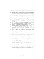
6.1.2 N-Version Programming with Tie-Breaker and Acceptance Test Example
This section provides an example implementation of the NVP-TB-AT tech-
nique. Recall the sort algorithm used in the RcB and NVP examples (see
Other Software Fault Tolerance Techniques 241
Sections 4.1.2 and 4.2.2, and Figure 4.2). The original sort implementation
produces incorrect results if one or more of the inputs are negative. The fol-
lowing describes how NVP-TB-AT can be used to protect the system against
faults arising from this error.
Figure 6.2 illustrates an NVP-TB-AT implementation of fault tol-
erance for this example. Note the additional components needed for
NVP-TB-AT implementation: an executive that handles orchestrating and
synchronizing the technique, two additional variants (versions) of the algo-
rithm/program, a comparator, a voter, and an AT. The versions are differ-
ent variants providing an incremental sort. For variants 1 and 2, a bubble
sort and quicksort are used, respectively. Variant 3 is the original incre-
mental sort.

Now, lets step through the example.
•
Upon entry to NVP-TB-AT, the executive performs the following:
formats calls to the n = 3 variants and through those calls distributes
the inputs to the variants. The input set is (8, 7, 13, −4, 17, 44). The
executive also sums the items in the input set for use in the AT. Sum
of input = 85.
•
Each variant, V
i
(i = 1, 2, 3), executes.
•
The results of the two fastest variant executions (R
ij
, i = 2, 3; j = 1,
…, k) are gathered by the executive and submitted to the comparator.
•
The comparator examines the results as follows (shading indicates
matching results):
j R
2j
R
3j
Result
1 −4 −4 −4
2 7 −7 Ø
3 8 −8 Ø
4 13 −13 Ø
5 17 −17 Ø
6 44 −44 Ø

The results do not match.
•
The executive now waits for the result of the slowest variant to com-
plete execution.
242 Software Fault Tolerance Techniques and Implementation
•
The slowest variant, V
1
, completes execution.
•
The result from the slowest variant, R
1
, is gathered by the executive
and, along with R
2
and R
3
, is submitted to the majority voter.
Other Software Fault Tolerance Techniques 243
(8, 7, 13, −4, 17, 44)
Variant 2:
Quicksort
Variant 3:
Original
incremental sort
Variant 1:
Bubble sort
Comparator:
Result no
match

=
(−4, 7, 8, 13, 17, 44)− − − − −
Output: (−4, 7, 8, 13, 17, 44)
R
2j
: −4 7 8 13 17 44
: 4 7 8 13 17 44R
3j
− − − − − −
R
R
1
3
j
j
: 4 7 8 13 17 44
4 7 8 13 17 44
: 4 7 8 13 17 44
−
− − − − − −
R
2j
: −
Sum of inputs = 85,
distribute inputs
Majority
voter: Result
and match
=
R R

1 2j j
R = −( 4, 7, 8, 13, 17, 44)
AT: Sum of inputs
sum of outputs
85=
=
(−4, 7, 8, 13, 17, 44)
(−4, 7, 8, 13, 17, 44)
Figu re 6.2 Example of N-version programming with tie-breaker and acceptance test
impl ementation.
•
The majority voter examines the results as follows (shading indicates
matching results):
j R
1j
R
2j
R
3j
Result
 −" −" −" −"
% % −% %
! & & −& &
" ! ! −! !
# % % −% %
$ "" "" −"" ""
R
1
and R
2

match, so the majority result is (−4, 7, 8, 13, 17, 44).
•
Control returns to the executive.
•
The executive submits the majority result to the AT.
• The AT sums the items in the output set. Sum of output = 85. The
AT tests if the sum of input equals the sum of output.85= 85, so the
majority result passes the AT.
•
Control returns to the executive.
•
The executive passes the presumed correct result, (−4, 7, 8, 13, 17,
44), outside the NVP-TB-AT, and the NVP-TB-AT module is
exited.
6.2 Resourceful Systems
Resourceful systems were proposed by Abbott [7, 8] as an approach to soft-
ware fault tolerance. It is an artificial intelligence approach, sometimes called
functional diversity, that exploits diversity in the functional space available
in some applications. The resourceful systems approach is based on self-
protective and self-checking components, and is derived from an approach
to fault tolerance in which system goals are made explicit. It was evolved
from the efforts of Taylor and Black [9] and Bastani and Yen [10], and work
in planning and robotics. Taylor and Blacks aim in [9] was to make goals
explicit for the sake of protecting the system from disaster, rather than for
reliability. Bastani and Yens work [10] focused on decentralized control,
244 Software Fault Tolerance Techniques and Implementation
rather than on system goals. Resourceful systems marry these ideas and
a plann ing component, yielding an extend ed RcB framework.
The resourceful system approach requires that system goals be made
explicit and that the system have the ability to achieve its goals in multiple

ways. A resourceful system, like a system using RcB, has the ability to deter-
mine whether it has achieved a goal (the goal must be testable) and, if it has
failed, to develop and carry out alternative plans for achieving the goal [8].
In an RcB, the alternatives are available prior to execution; however, in the
resourceful system the new ways to reach the goal may be generated dur-
ing execution. Hence, resourceful systems may generate new code dynami-
cally. (Obviously, dynamic code generation raises additional questions as to
whether the autogenerated code is safe (in the systems context) and whether
the code generator itself is dependable. These issues require additional inves-
tigation.) The resourceful system approach is based on the premise that,
although the system may fail to achieve the final goal in its primary or initial
way, the system may be able to achieve the goal in another way by modifying
plans and operations (see Figure 6.3). Associated with the goal may be con-
straints such as within x time units or within k iterations.
Systems using RcB may be viewed as a limited form of resourcefulness,
and resourceful systems may be viewed as a generalization of the RcB
approach [8].
Abbott, in [8], provides the following properties a resourceful system
must possess.
Other Software Fault Tolerance Techniques 245
Yes
No
Execute a
plan
Goal
achieved?
Modify plan,
generate
code
Figu re 6.3 General concept of a resourceful system.

•
Functional richness: The required redundancy is in the end results; it
is only necessary that it be possible to achieve the same end results in
a number of different ways. Functional richness is a property of a
system in the context of the environment in which it is functioning,
not of the system in isolation.
•
Explicitly testable goals: The system must be able to determine
whether or not it has achieved its goals. This is similar to the need
for ATs in an RcB technique.
•
An ability to develop and carry out plans for achieving its goals: The
system must be able to reason about its goals well enough to make
use of its functional richness. The required reasoning ability must
complement the systems functionality. The system must be able
to decompose its goals into subgoals in ways that correspond to the
ways it has of achieving those goals.
What is desired for a resourceful system is a broad set of basic functions
along with the ability to combine those functions into programs or plans. In
other words, one wants a system organized into levels of abstraction, where
each level provides the functional richness needed by the potential programs
on the next higher level of abstraction. The system itself does the program-
ming, that is, the planning and reacting, to deal with contingencies as they
arise [8].
Abbott contends that resourceful systems would be affordable because
functional richness grows out of a levels-of-abstraction object-oriented (OO)
approach to system design [8]. He adds that OO designs do not appear to
impose a significant cost penalty and may result in less expensive systems in
the long run.
Artificial intelligence techniques are used by the system to reason about

its goals, to devise methods of accomplishing the task, and to develop and
carry out plans for achieving its goals. The resourceful system approach tends
to change the way one views the relationships among a system, its environ-
ment, and the goals the system is intended to achieve. These altered views are
presented by Abbott [8] as follows.
•
The boundary between the system and the environment is less
distinct.
246 Software Fault Tolerance Techniques and Implementation
TEAMFLY























































Team-Fly
®

•
The systems goals become that of guiding the system and environ-
ment as an ensemble to assume a desired state, rather than to per-
form a function in, on, or to the environment.
•
System component failures are seen more as additional obstacles to
be overcome than as losses in functionality.
The following are important features for any language used for pro-
grams that control the operation of resourceful systems [8], but not necessar-
ily the language in which the system itself is implemented.
•
Components;
•
Ability to express the information to be checked;
•
Error reporting mechanism;
• Planning capability;
• Ability to generate and execute new code dynamically.
Abbott asserts (in [8 ]) that the technology needed for providing a
dynamic debugging (i.e., automatic detection and correction of bugs) capa-
bility is essentially the same as that of program verification and that in 1990
the technology was not suitable for general application. This is still the case
today. It is also asserted [8] that logic programming (e.g., using the Prolog
language) offers the best available language resources for developing fault-

tolerant software. The application areas in which resourcefulness has been
most fully developed are robotics and game playing systems. Intelligent agent
technology may hold promise for implementing resourceful systems [11].
The resourceful system approach to software fault tolerance still suffers the
same problems as all new approaches, that is, lack of testing, experimental
evaluation, implementation, and independent analysis.
6.3 Data-Driven Dependability Assurance Scheme
The data-driven dependability assurance scheme was developed by Parhami
[12, 13]. This approach is based on attaching dependability tags (d-tag) to
data objects and updating the d-tags as computation progresses. A d-tag is
an indicator of the probability of correctness of a data object. For software
fault tolerance use, the d-tag value for a particular data object can be used to
Other Software Fault Tolerance Techniques "%
determine the acceptability of that data object or can be used in more com-
plex decision-making functions.
Let a data object, D, and its d-tag comprise the composite object,
〈D, d 〉. The d-tag, d, assumes values from a finite set of dependability indica-
tors, d ∈ {0, 1, …, @ − 1}, where @ is an application-dependent constant.
Each d-tag value, d, has the constants,
F
@
and
′
F
@
, associated with it such
that the probability that the data object, D, is correct is bounded by these
constants:
F
@

≤ prob[D is correct] ≤
′
F
@
The d-tag values are arranged so that a larger d-tag value implies higher con-
fidence in the correctness of the associated data object. The d-tag values are
obtained from knowledge of the data and the application. We let the upper
bound,
′
= =
−
F F
@
j
1
1
, that is, a perfect value, and the lower bound,
F
0
be 0,
a hopelessly incorrect value.
The F
j
values are not required to conform to any particular rule or
pattern. In practice, though, it is desirable to have a capability for greater
discrimination at the high end of dependability values [12]. The reasoning
for this is that correctness probabilities 0.99 and 0.999 are significantly dif-
ferent, while the values 0.4 and 0.5 are not, because they both represent prac-
tically useless data values. The following example illustrates 8-valued d-tags
(@ = 8) [12]:

j: 0 1 2 3 4 5 6 7
π
j
: 0 0.75 0.883 0.9612 0.9894 0.9973 0.9999 1
The d-tags can be associated with data objects at any level; however, practical
considerations (e.g., data storage redundancy, and computational overhead)
will likely restrict their use to high-level data objects with complex structures
and operations.
The d-tags are manipulated, as the computation progresses, to indicate
the dependability of the data object. Normal operations on data objects (such
as multiplicati on, divi sion, ad dition, subtraction, et c.) tend t o lower th e
value of the d-tag. If it can be reasonably assumed that the operations them-
selves are perfectly dependable, then the dependability of each result of an
operation is a function of the operands dependabilities. With a unary opera-
tor then, the dependability of the result would be the same as that of the sin-
gle operand. Parhami [13] extends this to the development of a dependability
248 Software Fault Tolerance Techniques and Implementation
evaluation function for binary operators, such that the dependability of the
result is never more than the smallest d-tag value involved in the operation.
If the final computation results have acceptable d-tag values, then noth-
ing further is required. However, if the resultant d-tags are below a required
minimum (e.g., using a bounds AT), then something must be done to
increase the dependability of the data object. These dependability-raising
operations are involved only as needed during or at the end of computation.
Results that are obtained in more than one way (e.g., using hardware,
software, or temporal redundancy) increase the value of the d-tag. That is,
they increase the probability of correctness of the data object. Parhami [13]
provides detailed derivation of the correctness probability of a data object D
obtained in two different ways. In general, it can be concluded from the deri-
vation that dependability improvement is likely as a result of matching values

of D as long as the associated d-tag values are sufficiently high [13].
The results are extended and generalized to n variant results. If all the
results are different, then the data object with the highest d-tag value can be
selected as the final result. This is illustrated in the top third of Figure 6.4.
If all of the data object values are the same, then the output is set to one
of them with a d-tag value functionally comprised of all the variant results
d-tag values (see middle portion of Figure 6.4). In the other case, if the data
objects can be partitioned into classes of identical objects, then a result can
be determined as follows. For each class of identical objects, a d-tag value
is computed. The class with the largest computed d-tag determines the
resultant output data value. This case is illustrated in the bottom section of
Figure 6.4.
The last case, in which some (but not a majority of) data objects are
identical, is perhaps best explained by an example. Suppose we have seven
variants (v
i
, i = 1, 2, …, 7), and these variants produce the data objects and
associated d-tags shown in Table 6.1.
There is no majority of identical data objects. However, there are
classes (subsets) of identical objects. The members of these classes are:
Class 1: 〈D
1
, d
1
〉, 〈D
6
, d
6
〉;
Class 2: (D

2
, d
2
〉, 〈D
4
, d
4
〉, 〈D
5
, d
5
〉;
Class 3: 〈D
3
, d
3
〉;
Class 4: 〈D
4
, d
4
〉.
To determine which result to use, class 1s data object value 10.7, class 2s
11.1, class 3s 42.9, or class 4s -3.6, a d-tag value must be determined for
Other Software Fault Tolerance Techniques "'
250 Software Fault Tolerance Techniques and Implementation
Case: All D
i
are different
Case: All D

i
are equal
Case: Some D
i
are equal
Variant 2 Variant n
Variant n

Variant 1
Variant 2

Variant 1
Variant 2 Variant nVariant 1
m classes of equivalent data objects
For each class, (d f d′ =
k i
), those data
objects within the class, 1, ,
i
k m
=
= …
Result , , where max( ), 1, ,= 〈 〉 = = …D d d d i n
j j j i
Result , , where max( ), 1, ,= 〈 ′〉 ′ = = …D d d d i m
j j j k
Result , , where ( ), 1, ,= 〈 〉 = = …D d d f d i n
j j j i

〈 〉D d

1 1
,
〈 〉D d
1 1
,
〈 〉D d
1 1
,
〈 〉D d
2 2
,
〈 〉D d
2 2
,
〈 〉D d
2 2
,
〈 〉D d
n n
,
〈 〉D d
n n
,
〈 〉D d
n n
,
D D D
1 2
≠ ≠ … ≠
n

D D D
1 2
= = … =
n
Figu re 6.4 Using d-tags with n variants to de termine result.
each class. Suppose the class d-tag values are simply the average of the d-tag
values associated with the data objects in each class. The class d-tag values are
provided below.
Class 1s d-tag value: d′
1
= avg(0.9886, 0.9940) = 0.9913
Class 2s d-tag value: d′
2
= avg(0.9984, 0.9946, 0.9986) = 0.9972
Class 3s d-tag value: d′
3
= avg(0.2111) = 0.2111
Class 4s d-tag value: d′
4
= avg(0.1234) = 0.1234
The result, in this example, will be the data object value of the class with the
maximum associated d-tag value.
max(d′
i
) = d′
2
, i = 1, 2, …, 7
So, the data object value associated with class 2, 11.1, is output as the pre-
sumed correct result.
There are several issues related to d-tags.

•
d-tag values: Determining the number and values of d-tags to use is
nontrivial. The number of d-tag intervals affects the storage and
processing overheads. The optimal number will be application
dependent. To effectively perform the trade-off analyses to determine
these numbers, the concept of d-tags and their associated direct and
indirect costs must be formalized and further refined [13].
Other Software Fault Tolerance Techniques #
Table 6.1
Example Data Ob ject and d-tag Values
Variant, E Data Object, ,
E
d-tag, @
E
1 10.7 0.9886
2 11.1 0.9984
3 42.9 0.2111
4 11.1 0.9946
5 11.1 0.9986
6 10.7 0.9940
7 −3.6 0.1234
•
Erroneous d-tags: The d-tags themselves may be incorrect and, hence,
lower or higher than the correct value. If the d-tag is lower than cor-
rect, then this error is safe because it can lead to the following
events [13]:
•
A correct result will have an erroneously low, but acceptable,
d-tag value and will be trusted and used;
•

A correct result will have an unacceptably low d-tag value and will
be either discarded or used cautiously;
•
Or, an incorrect result will have a correct d-tag and will be either
discarded or used with appropriate care.
Hence, it is sufficient to guard against erroneously high d-tag values.
These positive d-tag errors have three causes:
•
Incorrect storage and/or transmission of d-tag values;
• Error(s) during dependability-lowering operations;
• Error(s) during dependability-raising operations.
Several means of combating these causes, including use of error
codes, exploiting asymmetry in the application, arithmetic error
codes, table look-up error codes, and self-checking circuits, are pro-
vided by Parhami [13].
•
Imperfect operations: Operators (e.g., +, −,/,∗) may be erroneous,
comparison and voting operations may be erroneous, and operators
may incorrectly operate on composite data objects.
Earlier in this section, we showed how to use d-tags with n variants
(design diversity) to determine the correct result. It is also possible to use
d-tags with data diverse techniques to determine the correct result. For exam-
ple, they can be added to the operation of the RtB technique and used in
voting on the result if the original computation and computation with
re-expressed inputs fail to pass the AT. In addition, d-tags can be added,
along with ATs and stepwise comparison, to the N-copy programming
(NCP) technique. Furthermore, d-tags can also be used with combined
design and data diverse techniques to aid in decision making and selective
use of redundancy (see [13] for details).
252 Software Fault Tolerance Techniques and Implementation

6.4 Self-Configuring Optimal Programming
SCOP, developed by Bondavalli, Di Giandomenico, and Xu [1417], is a
scheme for handling dependability and efficiency. SCOP attempts to reduce
the cost of fault-tolerant software in terms of space and time redundancy
by providing a flexible redundancy architecture. Within this architecture,
dependability and efficiency can be dynamically adjusted at run time.
The SCOP technique uses n software variants, a DM (Section 7.1), a
controller or executive, and forward recovery (Section 1.4.2) to accomplish
fault tolerance. The main characteristics of SCOP are dynamic use of redun-
dancy, growing syndrome space (collection of information to support result
selection), flexibility and efficiency, and generality. These characteristics will
be described in the SCOP operation discussion.
SCOP operation is described in Section 6.4.1, with an example pro-
vided in Section 6.4.2. Some issues and SCOP evaluation are presented in
Section 6.4.3.
6.4.1 Self-Configuring Optimal Programming Operation
The SCOP technique consists of an executive or controller, n variants of the
program or function, and a DM. The controller orchestrates the SCOP tech-
nique operation, which follows the algorithm below.
Index_of_Current_Phase = 0
Current_State = non_end_state
Syndrome = empty
Delivery_Condition = one of {Possible_Delivery_Conditions}
Max_Number_Phases = f[Time_Constraints]
while ((Current_State ≠ non_end_state) AND
(Index_of_Current_Phase < Max_Number_Phases))
begin
Index_of_Current_Phase = Index_of_Current_Phase + 1
construct Currently_Active_Set_of_Variants
execute (Currently_Active_Set_of_Variants,

New_Syndrome)
adjudicate (Currently_Active_Set_of_Variants,
All_Syndromes, New_State, Result)
Current_State = New_State
end
if (Current_State = end_state)
then deliver(Result)
else signal(failure)
Other Software Fault Tolerance Techniques #!
The SCOP control algorithm [17] above states that first some initiali-
zations take place: the current phase number is set to 0, the current state is set
to a non-end state (which is also a nonfailure state), and the information syn-
drome is cleared. In the SCOP technique, an information syndrome contains
the variant results and an indication of each results correctness. The delivery
condition is set next. SCOP provides different levels of dependability based
on the selected delivery condition. Different delivery conditions usually have
different fault coverages and can be chosen, statically or dynamically, based
on the application criticality or system degradation, for example. The maxi-
mum number of phases is determined next. Its value is based on time con-
straints and the expected time per phase.
The first phase is initiated. Additional phases will be performed as long
as the maximum number of phases is not exceeded and the current state of
the system is not an end state. Upon starting the phase, the phase counter is
incremented. The initial currently active set (CAS) of variants, V
1
, is con-
structed according to the selected delivery condition and the given applica-
tion environment. In subsequent phases, the CAS set V
i
(i > 1) is constructed

based on the syndrome S
i − 1
collected in the (i − 1)th phase and the infor-
mation on phases [17]. The variants in V
i
are selected from the variants
that have not been used in any of the previous phases; that is, V
i
is a subset of
V − (V
1
∪ V
2
∪ … ∪ V
i − 1
). If the ith phase is the last, V
i
would contain all
the remaining spare variants [17].
The
execute procedure manages the execution of the CAS variants
and generates the syndrome S
i
(where S
0
is an empty set and S
i − 1
is a subset
of S
i

). The adjudication function is based on the selected delivery condition.
The adjudicator receives the syndrome S
i
, then, based on its result, sets the
new state and selects the result if one exists. When the current state is the end
state, the selected result is delivered or a failure notification is signaled.
Figure 6.5 (based on information in [17]) illustrates the structure and
operation of the SCOP technique in a multiprocessor environment. In the
description of the figure and the operation of SCOP below, the following
variables are used:
C Delivery condition;
CAS Currently active set (of variants);
i Phase number;
N
p
Maximum number of software variants that can be executed
in parallel on hardware resources currently allocated to the
given application;
254 Software Fault Tolerance Techniques and Implementation
Other Software Fault Tolerance Techniques 255
User requirements SCOP
Deliver presumably
correct result
SCOP exit
Exception OR
degraded service
Input
1
2
N

p
variants
are executed.
Modify V
i
No
Yes
3
No
Yes
4
No
Yes
Wait
6
Generate S
i
7
Is C
satisfied?
8
No
Yes
i i: 1= +
Construct V
i
9
5
i T
V

V C
: 1; set
Construct such that
may satisfy
=
 
d
1
1
V T
i d
{ } AND≠
satisfied if Phase ?i
N
p
0?>
  >V N
i p
?
 V
i
or more
variants are
executed
Figu re 6.5 Self-configuring optimal programming str ucture and operation. (After: [17],
© 1995 Springer-Verlag, Figure 2, p. 161.)