CHAPTER 2. CONVOLUTIONS 44
+ 0 1 2 3 4 5 6 7 8 9 10 11 12 13 14 15
|
0: 0 1 2 3 4 5 6 7 8 9 10 11 12 13 14 15
1: 1 2 3 4 5 6 7 8 9 10 11 12 13 14 15 0-
2: 2 3 4 5 6 7 8 9 10 11 12 13 14 15 0- 1-
3: 3 4 5 6 7 8 9 10 11 12 13 14 15 0- 1- 2-
4: 4 5 6 7 8 9 10 11 12 13 14 15 0- 1- 2- 3-
5: 5 6 7 8 9 10 11 12 13 14 15 0- 1- 2- 3- 4-
6: 6 7 8 9 10 11 12 13 14 15 0- 1- 2- 3- 4- 5-
7: 7 8 9 10 11 12 13 14 15 0- 1- 2- 3- 4- 5- 6-
8: 8 9 10 11 12 13 14 15 0- 1- 2- 3- 4- 5- 6- 7-
9: 9 10 11 12 13 14 15 0- 1- 2- 3- 4- 5- 6- 7- 8-
10: 10 11 12 13 14 15 0- 1- 2- 3- 4- 5- 6- 7- 8- 9-
11: 11 12 13 14 15 0- 1- 2- 3- 4- 5- 6- 7- 8- 9- 10-
12: 12 13 14 15 0- 1- 2- 3- 4- 5- 6- 7- 8- 9- 10- 11-
13: 13 14 15 0- 1- 2- 3- 4- 5- 6- 7- 8- 9- 10- 11- 12-
14: 14 15 0- 1- 2- 3- 4- 5- 6- 7- 8- 9- 10- 11- 12- 13-
15: 15 0- 1- 2- 3- 4- 5- 6- 7- 8- 9- 10- 11- 12- 13- 14-
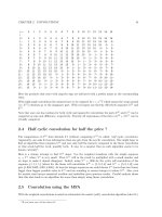
Here the products that enter with negative sign are indicated with a postfix minus at the corresponding
entry.
With right-angle convolution the minuses have to be replaced by i =
√
−1 which means the wrap-around
(i.e. h
(1)
) elements go to the imaginary part. With real input one thereby effectively separates h
(0)
and
h
(1)

.
Note that once one has routines for both cyclic and negacyclic convolution the parts h
(0)
and h
(1)
can be
computed as sum and difference, respectively. Thereby all expressions of the form α h
(0)
+ β h
(1)
can be
trivially computed.
2.4 Half cyclic convolution for half the price ?
The computation of h
(0)
from formula 2.7 (without computing h
(1)
) is called half cyclic convolution.
Apparently, one asks for less information than one gets from the acyclic convolution. One might hope to
find an algorithm that computes h
(0)
and uses only half the memory compared to the linear convolution
or that needs half the work, possibly both. It may be a surprise that no such algorithm seems to be
known currently
5
.
Here is a clumsy attempt to find h
(0)
alone: Use the weighted transform with the weight sequence
v

x
= V
x
where V
n
is very small. Then h
(1)
will in the result be multiplied with a small number and
we hope to make it almost disappear. Indeed, using V
n
= 1000 for the cyclic self convolution of the
sequence {1, 1, 1, 1} (where for the linear self convolution h
(0)
= {1, 2, 3, 4} and h
(1)
= {3, 2, 1, 0}) one
gets {1.003, 2.002, 3.001, 4.000}. At least for integer sequences one could choose V
n
(more than two times)
bigger than biggest possible value in h
(1)
and use rounding to nearest integer to isolate h
(0)
. Alas, even
for modest sized arrays numerical overflow and underflow gives spurious results. Careful analysis shows
that this idea leads to an algorithm far worse than simply using linear convolution.
2.5 Convolution using the MFA
With the weighted convolutions in mind we reformulate the matrix (self-) convolution algorithm (idea 2.1):
5
If you know one, tell me about it!

CHAPTER 2. CONVOLUTIONS 45
1. Apply a FFT on each column.
2. On each row apply the weighted convolution with V
C
= e
2 π i r/R
= 1
r/R
where R is the total
numb er of rows, r = 0 R − 1 the index of the row, C the length of each row (or, equivalently the
total numb er columns)
3. Apply a FFT on each column (of the transposed matrix).
First consider
2.5.1 The case R = 2
The cyclic auto convolution of the sequence x can be obtained by two half length convolutions (one cyclic,
one negacyclic) of the sequences
6
s := x
(0/2)
+ x
(1/2)
and d := x
(0/2)
− x
(1/2)
using the formula
x  x =
1
2
{s  s + d 

−
d, s  s −d 
−
d} (2.20)
The equivalent formula for the cyclic convolution of two sequences x and y is
x  y =
1
2
{s
x
 s
y
+ d
x

−
d
y
, s
x
 s
y
− d
x

−
d
y
} (2.21)
where

s
x
:= x
(0/2)
+ x
(1/2)
d
x
:= x
(0/2)
− x
(1/2)
s
y
:= y
(0/2)
+ y
(1/2)
d
y
:= y
(0/2)
− y
(1/2)
For the acyclic (or linear) convolution of sequences one can use the cyclic convolution of the zero padded
sequences z
x
:= {x
0
, x

1
, . . . , n
n−1
, 0, 0, . . . , 0} (i.e. x with n zeros appended). Using formula 2.20 one gets
for the two sequences x and y (with s
x
= d
x
= x, s
y
= d
y
= y):
x 
ac
y = z
x
 z
y
=
1
2
{x  y + x 
−
y, x  y − x 
−
y} (2.22)
And for the acyclic auto convolution:
x 
ac

x = z  z =
1
2
{x  x + x 
−
x, x  x −x 
−
x} (2.23)
2.5.2 The case R = 3
Let ω =
1
2
(1 +
√
3) and define
A := x
(0/3)
+ x
(1/3)
+ x
(2/3)
B := x
(0/3)
+ ω x
(1/3)
+ ω
2
x
(2/3)
C := x

(0/3)
+ ω
2
x
(1/3)
+ ω x
(2/3)
Then, if h := x 
ac
x, there is
x
(0/3)
= A  A + B 
{ω}
B + C 
{ω
2
}
C (2.24)
x
(1/3)
= A  A + ω
2
(B 
{ω }
B) + ω (C 
{ω
2
}
C)

x
(2/3)
= A  A + ω (B 
{ω}
B) + ω
2
(C 
{ω
2
}
C)
For real valued data C is the complex conjugate (cc.) of B and (with ω
2
= cc.ω) B 
{ω }
B is the cc. of
C 
{ω
2
}
C and therefore every B 
{}
B-term is the cc. of the C 
{}
C-term in the same line. Is there a nice
and general scheme for real valued convolutions based on the MFA? Read on for the positive answer.
6
s, d lower half plus/minus higher half of x
CHAPTER 2. CONVOLUTIONS 46
2.6 Convolution of real valued data using the MFA

For row 0 (which is real after the column FFTs) one needs to compute the (usual) cyclic convolution; for
row R/2 (also real after the column FFTs) a negacyclic convolution is needed
7
, the code for that task is
given on page 62.
All other weighted convolutions involve complex computations, but it is easy to see how to reduce the
work by 50 percent: As the result must b e real the data in row number R − r must, because of the
symmetries of the real and imaginary part of the (inverse) Fourier transform of real data, be the complex
conjugate of the data in row r. Therefore one can use real FFTs (R2CFTs) for all column-transforms for
step 1 and half-complex to real FFTs (C2RFTs) for step 3.
Let the computational cost of a cyclic (real) convolution be q, then
For R even one must perform 1 cyclic (row 0), 1 negacyclic (row R/2) and R/2 − 2 complex (weighted)
convolutions (rows 1, 2, . . . , R/2 −1)
For R odd one must perform 1 cyclic (row 0) and (R − 1)/2 complex (weighted) convolutions (rows
1, 2, . . . , (R −1)/2)
Now assume, slightly simplifying, that the cyclic and the negacyclic real convolution involve the same
numb er of computations and that the cost of a weighted complex convolution is twice as high. Then in
both cases ab ove the total work is exactly half of that for the complex case, which is ab out what one
would expect from a real world real valued convolution algorithm.
For acyclic convolution one may want to use the right angle convolution (and complex FFTs in the column
passes).
2.7 Convolution without transposition using the MFA
Section 8.4 explained the connection between revbin-permutation and transposition. Equipped with that
knowledge an algorithm for convolution using the MFA that uses revbin_permute instead of transpose
is almost straight forward:
rows=8 columns=4
input data (symbolic format: R00C):
0: 0 1 2 3
1: 1000 1001 1002 1003
2: 2000 2001 2002 2003

3: 3000 3001 3002 3003
4: 4000 4001 4002 4003
5: 5000 5001 5002 5003
6: 6000 6001 6002 6003
7: 7000 7001 7002 7003
FULL REVBIN_PERMUTE for transposition:
0: 0 4000 2000 6000 1000 5000 3000 7000
1: 2 4002 2002 6002 1002 5002 3002 7002
2: 1 4001 2001 6001 1001 5001 3001 7001
3: 3 4003 2003 6003 1003 5003 3003 7003
DIT FFTs on revbin_permuted rows (in revbin_permuted sequence), i.e. unrevbin_permute rows:
(apply weight after each FFT)
0: 0 1000 2000 3000 4000 5000 6000 7000
1: 2 1002 2002 3002 4002 5002 6002 7002
2: 1 1001 2001 3001 4001 5001 6001 7001
7
For R odd there is no such row and no negacyclic convolution is needed.
CHAPTER 2. CONVOLUTIONS 47
3: 3 1003 2003 3003 4003 5003 6003 7003
FULL REVBIN_PERMUTE for transposition:
0: 0 1 2 3
1: 4000 4001 4002 4003
2: 2000 2001 2002 2003
3: 6000 6001 6002 6003
4: 1000 1001 1002 1003
5: 5000 5001 5002 5003
6: 3000 3001 3002 3003
7: 7000 7001 7002 7003
CONVOLUTIONS on rows (do not care revbin_permuted sequence), no reordering.
FULL REVBIN_PERMUTE for transposition:

0: 0 1000 2000 3000 4000 5000 6000 7000
1: 2 1002 2002 3002 4002 5002 6002 7002
2: 1 1001 2001 3001 4001 5001 6001 7001
3: 3 1003 2003 3003 4003 5003 6003 7003
(apply inverse weight before each FFT)
DIF FFTs on rows (in revbin_permuted sequence), i.e. revbin_permute rows:
0: 0 4000 2000 6000 1000 5000 3000 7000
1: 2 4002 2002 6002 1002 5002 3002 7002
2: 1 4001 2001 6001 1001 5001 3001 7001
3: 3 4003 2003 6003 1003 5003 3003 7003
FULL REVBIN_PERMUTE for transposition:
0: 0 1 2 3
1: 1000 1001 1002 1003
2: 2000 2001 2002 2003
3: 3000 3001 3002 3003
4: 4000 4001 4002 4003
5: 5000 5001 5002 5003
6: 6000 6001 6002 6003
7: 7000 7001 7002 7003
As shown works for sizes that are a power of two, generalizes for sizes a power of some prime. TBD: add
text
2.8 The z-transform (ZT)
In this section we will learn a technique to compute the FT by a (linear) convolution. In fact, the
transform computed is the z-transform, a more general transform that in a special case is identical to the
FT.
2.8.1 Definition of the ZT
The z-transform (ZT) Z [a] = ˆa of a (length n) sequence a with elements a
x
is defined as
ˆa

k
:=
n−1

x=0
a
x
z
k x
(2.25)
The z-transform is a linear transformation, its most important property is the convolution property
CHAPTER 2. CONVOLUTIONS 48
(formula 2.3): Convolution in original space corresponds to ordinary (elementwise) multiplication in
z-space. (See [10] and [11].)
Note that the special case z = e
±2 π i/n
is the discrete Fourier transform.
2.8.2 Computation of the ZT via convolution
In the definition of the (discrete) z-transform we rewrite
8
the product x k as
x k =
1
2

x
2
+ k
2
− (k − x)

2

(2.26)
ˆ
f
k
=
n−1

x=0
f
x
z
x k
= z
k
2
/2
n−1

x=0

f
x
z
x
2
/2

z

−(k−x)
2
/2
(2.27)
This leads to the following
Idea 2.2 (chirp z-transform) Algorithm for the chirp z-transform:
1. Multiply f elementwise with z
x
2
/2
.
2. Convolve (acyclically) the resulting sequence with the sequence z
−x
2
/2
, zero padding of the sequences
is required here.
3. Multiply elementwise with the sequence z
k
2
/2
.
The above algorithm constitutes a ‘fast’ (∼ n log(n)) algorithm for the ZT because fast convolution is
possible via FFT.
2.8.3 Arbitrary length FFT by ZT
We first note that the length n of the input sequence a for the fast z-transform is not limited to highly
composite values (especially n prime is allowed): For values of n where a FFT is not feasible pad the
sequence with zeros up to a length L with L >= 2 n and a length L FFT becomes feasible (e.g. L is a
power of 2).
Second remember that the FT is the special case z = e

±2 π i/n
of the ZT: With the chirp ZT algorithm
one also has an (arbitrary length) FFT algorithm
The transform takes a few times more than an optimal transform (by direct FFT) would take. The worst
case (if only FFTs for n a power of 2 are available) is n = 2
p
+ 1: One must perform 3 FFTs of length
2
p+2
≈ 4 n for the computation of the convolution. So the total work amounts to about 12 times the
work a FFT of length n = 2
p
would cost. It is of course possible to lower this ‘worst case factor’ to 6 by
using highly composite L slightly greater than 2 n.
[FXT: fft arblen in chirp/fftarblen.cc]
TBD: show shortcuts for n even/odd
2.8.4 Fractional Fourier transform by ZT
The z-transform with z = e
α 2 π i/n
and α = 1 is called the fractional Fourier transform (FRFT). Uses of
the FRFT are e.g. the computation of the DFT for data sets that have only few nonzero elements and the
detection of frequencies that are not integer multiples of the lowest frequency of the DFT. A thorough
discussion can be found in [35].
[FXT: fft fract in chirp/fftfract.cc]
8
cf. [2]
Chapter 3
The Hartley transform (HT)
3.1 Definition of the HT
The Hartley transform (HT) is defined like the Fourier transform with ‘cos + sin’ instead of ‘cos +i ·sin’.

The (discrete) Hartley transform of a is defined as
c = H[a] (3.1)
c
k
:=
1
√
n
n−1

x=0
a
x

cos
2 π k x
n
+ sin
2 π k x
n

(3.2)
It has the obvious property that real input produces real output,
H[a] ∈ R for a ∈ R (3.3)
It also is its own inverse:
H[H[a]] = a (3.4)
The symmetries of the HT are simply:
H[a
S
] = H[a

S
] = H[a
S
] (3.5)
H[a
A
] = H[a
A
] = −H[a
A
] (3.6)
i.e. symmetry is, like for the FT, conserved.
3.2 radix 2 FHT algorithms
3.2.1 Decimation in time (DIT) FHT
For a sequence a of length n let X
1/2
a denote the sequence with elements a
x
cos π x/n + a
x
sin π x/n
(this is the ‘shift operator’ for the Hartley transform).
Idea 3.1 (FHT radix 2 DIT step) Radix 2 decimation in time step for the FHT:
H[a]
(left)
n/2
= H

a
(even)


+ X
1/2
H

a
(odd)

(3.7)
H[a]
(right)
n
n/2
= H

a
(even)

− X
1/2
H

a
(odd)

(3.8)
49
CHAPTER 3. THE HARTLEY TRANSFORM (HT) 50
Code 3.1 (recursive radix 2 DIT FHT) Pseudo code for a recursive procedure of the (radix 2) DIT
FHT algorithm:

procedure rec_fht_dit2(a[], n, x[])
// real a[0 n-1] input
// real x[0 n-1] result
{
real b[0 n/2-1], c[0 n/2-1] // workspace
real s[0 n/2-1], t[0 n/2-1] // workspace
if n == 1 then
{
x[0] := a[0]
return
}
nh := n/2;
for k:=0 to nh-1
{
s[k] := a[2*k] // even indexed elements
t[k] := a[2*k+1] // odd indexed elements
}
rec_fht_dit2(s[], nh, b[])
rec_fht_dit2(t[], nh, c[])
hartley_shift(c[], nh, 1/2)
for k:=0 to nh-1
{
x[k] := b[k] + c[k];
x[k+nh] := b[k] - c[k];
}
}
[source file: recfhtdit2.spr]
[FXT: recursive dit2 fht in slow/recfht2.cc]
The procedure hartley_shift replaces element c
k

of the input sequence c by c
k
cos(π k/n) +
c
n−k
sin(π k/n). Here is the pseudo code:
Code 3.2 (Hartley shift) procedure hartley_shift_05(c[], n)
// real c[0 n-1] input, result
{
nh := n/2
j := n-1
for k:=1 to nh-1
{
c := cos( PI*k/n )
s := sin( PI*k/n )
{c[k], c[j]} := {c[k]*c+c[j]*s, c[k]*s-c[j]*c}
j := j-1
}
}
[source file: hartleyshift.spr]
[FXT: hartley shift 05 in fht/hartleyshift.cc]
Code 3.3 (radix 2 DIT FHT, localized) Pseudo code for a non-recursive procedure of the (radix 2)
DIT FHT algorithm:
procedure fht_dit2(a[], ldn)
// real a[0 n-1] input,result
{
n := 2**ldn // length of a[] is a power of 2
revbin_permute(a[], n)
for ldm:=1 to ldn
{

m := 2**ldm
mh := m/2
m4 := m/4
CHAPTER 3. THE HARTLEY TRANSFORM (HT) 51
for r:=0 to n-m step m
{
for j:=1 to m4-1 // hartley_shift(a+r+mh,mh,1/2)
{
k := mh - j
u := a[r+mh+j]
v := a[r+mh+k]
c := cos(j*PI/mh)
s := sin(j*PI/mh)
{u, v} := {u*c+v*s, u*s-v*c}
a[r+mh+j] := u
a[r+mh+k] := v
}
for j:=0 to mh-1
{
u := a[r+j]
v := a[r+j+mh]
a[r+j] := u + v
a[r+j+mh] := u - v
}
}
}
}
[source file: fhtdit2.spr]
The derivation of the ‘usual’ DIT2 FHT algorithm starts by fusing the shift with the sum/diff step:
void dit2_fht_localized(double *f, ulong ldn)

{
const ulong n = 1<<ldn;
revbin_permute(f, n);
for (ulong ldm=1; ldm<=ldn; ++ldm)
{
const ulong m = (1<<ldm);
const ulong mh = (m>>1);
const ulong m4 = (mh>>1);
const double phi0 = M_PI/mh;
for (ulong r=0; r<n; r+=m)
{
{ // j == 0:
ulong t1 = r;
ulong t2 = t1 + mh;
sumdiff(f[t1], f[t2]);
}
if ( m4 )
{
ulong t1 = r + m4;
ulong t2 = t1 + mh;
sumdiff(f[t1], f[t2]);
}
for (ulong j=1, k=mh-1; j<k; ++j, k)
{
double s, c;
SinCos(phi0*j, &s, &c);
ulong tj = r + mh + j;
ulong tk = r + mh + k;
double fj = f[tj];
double fk = f[tk];

f[tj] = fj * c + fk * s;
f[tk] = fj * s - fk * c;
ulong t1 = r + j;
ulong t2 = tj; // == t1 + mh;
sumdiff(f[t1], f[t2]);
t1 = r + k;
t2 = tk; // == t1 + mh;
sumdiff(f[t1], f[t2]);
CHAPTER 3. THE HARTLEY TRANSFORM (HT) 52
}
}
}
}
[FXT: dit2 fht localized in fht/fhtdit2.cc] Swapping the innermost loops then yields (considerations
as for DIT FFT, page 13, hold)
void dit2_fht(double *f, ulong ldn)
// decimation in time radix 2 fht
{
const ulong n = 1<<ldn;
revbin_permute(f, n);
for (ulong ldm=1; ldm<=ldn; ++ldm)
{
const ulong m = (1<<ldm);
const ulong mh = (m>>1);
const ulong m4 = (mh>>1);
const double phi0 = M_PI/mh;
for (ulong r=0; r<n; r+=m)
{
{ // j == 0:
ulong t1 = r;

ulong t2 = t1 + mh;
sumdiff(f[t1], f[t2]);
}
if ( m4 )
{
ulong t1 = r + m4;
ulong t2 = t1 + mh;
sumdiff(f[t1], f[t2]);
}
}
for (ulong j=1, k=mh-1; j<k; ++j, k)
{
double s, c;
SinCos(phi0*j, &s, &c);
for (ulong r=0; r<n; r+=m)
{
ulong tj = r + mh + j;
ulong tk = r + mh + k;
double fj = f[tj];
double fk = f[tk];
f[tj] = fj * c + fk * s;
f[tk] = fj * s - fk * c;
ulong t1 = r + j;
ulong t2 = tj; // == t1 + mh;
sumdiff(f[t1], f[t2]);
t1 = r + k;
t2 = tk; // == t1 + mh;
sumdiff(f[t1], f[t2]);
}
}

}
}
[FXT: dit2 fht in fht/fhtdit2.cc]
3.2.2 Decimation in frequency (DIF) FHT
Idea 3.2 (FHT radix 2 DIF step) Radix 2 decimation in frequency step for the FHT:
H[a]
(even)
n/2
= H

a
(left)
+ a
(right)

(3.9)
H[a]
(odd)
n/2
= H

X
1/2

a
(left)
− a
(right)

(3.10)

CHAPTER 3. THE HARTLEY TRANSFORM (HT) 53
Code 3.4 (recursive radix 2 DIF FHT) Pseudo code for a recursive procedure of the (radix 2) DIF
FHT algorithm:
procedure rec_fht_dif2(a[], n, x[])
// real a[0 n-1] input
// real x[0 n-1] result
{
real b[0 n/2-1], c[0 n/2-1] // workspace
real s[0 n/2-1], t[0 n/2-1] // workspace
if n == 1 then
{
x[0] := a[0]
return
}
nh := n/2;
for k:=0 to nh-1
{
s[k] := a[k] // ’left’ elements
t[k] := a[k+nh] // ’right’ elements
}
for k:=0 to nh-1
{
{s[k], t[k]} := {s[k]+t[k], s[k]-t[k]}
}
hartley_shift(t[], nh, 1/2)
rec_fht_dif2(s[], nh, b[])
rec_fht_dif2(t[], nh, c[])
j := 0
for k:=0 to nh-1
{

x[j] := b[k]
x[j+1] := c[k]
j := j+2
}
}
[source file: recfhtdif2.spr]
[FXT: recursive dif2 fht in slow/recfht2.cc]
Code 3.5 (radix 2 DIF FHT, localized) Pseudo code for a non-recursive procedure of the (radix 2)
DIF FHT algorithm:
procedure fht_dif2(a[], ldn)
// real a[0 n-1] input,result
{
n := 2**ldn // length of a[] is a power of 2
for ldm:=ldn to 1 step -1
{
m := 2**ldm
mh := m/2
m4 := m/4
for r:=0 to n-m step m
{
for j:=0 to mh-1
{
u := a[r+j]
v := a[r+j+mh]
a[r+j] := u + v
a[r+j+mh] := u - v
}
for j:=1 to m4-1
{
k := mh - j

u := a[r+mh+j]
v := a[r+mh+k]
c := cos(j*PI/mh)
CHAPTER 3. THE HARTLEY TRANSFORM (HT) 54
s := sin(j*PI/mh)
{u, v} := {u*c+v*s, u*s-v*c}
a[r+mh+j] := u
a[r+mh+k] := v
}
}
}
revbin_permute(a[], n)
}
[source file: fhtdif2.spr]
[FXT: dif2 fht localized in fht/fhtdif2.cc]
The ‘usual’ DIF2 FHT algorithm then is
void dif2_fht(double *f, ulong ldn)
// decimation in frequency radix 2 fht
{
const ulong n = (1<<ldn);
for (ulong ldm=ldn; ldm>=1; ldm)
{
const ulong m = (1<<ldm);
const ulong mh = (m>>1);
const ulong m4 = (mh>>1);
const double phi0 = M_PI/mh;
for (ulong r=0; r<n; r+=m)
{
{ // j == 0:
ulong t1 = r;

ulong t2 = t1 + mh;
sumdiff(f[t1], f[t2]);
}
if ( m4 )
{
ulong t1 = r + m4;
ulong t2 = t1 + mh;
sumdiff(f[t1], f[t2]);
}
}
for (ulong j=1, k=mh-1; j<k; ++j, k)
{
double s, c;
SinCos(phi0*j, &s, &c);
for (ulong r=0; r<n; r+=m)
{
ulong tj = r + mh + j;
ulong tk = r + mh + k;
ulong t1 = r + j;
ulong t2 = tj; // == t1 + mh;
sumdiff(f[t1], f[t2]);
t1 = r + k;
t2 = tk; // == t1 + mh;
sumdiff(f[t1], f[t2]);
double fj = f[tj];
double fk = f[tk];
f[tj] = fj * c + fk * s;
f[tk] = fj * s - fk * c;
}
}

}
revbin_permute(f, n);
}
[FXT: dif2 fht in fht/fhtdif2.cc]
TBD: higher radix FHT
CHAPTER 3. THE HARTLEY TRANSFORM (HT) 55
3.3 Complex FT by HT
The relations between the HT and the FT can be read off directly from their definitions and their
symmetry relations. Let σ be the sign of the exponent in the FT, then the HT of a complex sequence
d ∈ C is:
F [d] =
1
2

H[d] + H[d] + σ i

H[d] −H[d]

(3.11)
Written out for the real and imaginary part d = a + i b (a, b ∈ R):
F [a + i b] =
1
2

H[a] + H[a] −σ

H[b] −H[b]

(3.12)
F [a + i b] =

1
2

H[b] + H[b] + σ

H[a] −H[a]

(3.13)
Alternatively, one can recast the relations (using the symmetry relations 3.5 and 3.6) as
F [a + i b] =
1
2
H[a
S
− σ b
A
] (3.14)
F [a + i b] =
1
2
H[b
S
+ σ a
A
] (3.15)
Both formulations lead to the very same
Code 3.6 (complex FT by HT conversion)
fht_fft_conversion(a[],b[],n,is)
// preprocessing to use two length-n FHTs
// to compute a length-n complex FFT

// or
// postprocessing to use two length-n FHTs
// to compute a length-n complex FFT
//
// self-inverse
{
for k:=1 to n/2-1
{
t := n-k
as := a[k] + a[t]
aa := a[k] - a[t]
bs := b[k] + b[t]
ba := b[k] - b[t]
aa := is * aa
ba := is * ba
a[k] := 1/2 * (as - ba)
a[t] := 1/2 * (as + ba)
b[k] := 1/2 * (bs + aa)
b[t] := 1/2 * (bs - aa)
}
}
[source file: fhtfftconversion.spr]
[FXT: fht fft conversion in fht/fhtfft.cc] [FXT: fht fft conversion in fht/fhtcfft.cc]
Now we have two options to compute a complex FT by two HTs:
Code 3.7 (complex FT by HT, version 1) Pseudo code for the complex Fourier transform that uses
the Hartley transform, is must be -1 or +1:
fft_by_fht1(a[],b[],n,is)
CHAPTER 3. THE HARTLEY TRANSFORM (HT) 56
// real a[0 n-1] input,result (real part)
// real b[0 n-1] input,result (imaginary part)

{
fht(a[], n)
fht(b[], n)
fht_fft_conversion(a[], b[], n, is)
}
and
Code 3.8 (complex FT by HT, version 2) Pseudo code for the complex Fourier transform that uses
the Hartley transform, is must be -1 or +1:
fft_by_fht2(a[],b[],n,is)
// real a[0 n-1] input,result (real part)
// real b[0 n-1] input,result (imaginary part)
{
fht_fft_conversion(a[], b[], n, is)
fht(a[], n)
fht(b[], n)
}
Note that the real and imaginary parts of the FT are computed independently by this procedure.
For convolutions it would be sensible to use procedure 3.7 for the forward and 3.8 for the backward
transform. The complex squarings are then combined with the pre- and postprocessing steps, thereby
interleaving the most nonlocal memory accesses with several arithmetic operations.
[FXT: fht fft in fht/fhtcfft.cc]
3.4 Complex FT by complex HT and vice versa
A complex valued HT is simply two HTs (one of the real, one of the imag part). So we can use both of
3.7 or 3.8 and there is nothing new. Really? If one writes a type complex version of both the conversion
and the FHT the routine 3.7 will look like
fft_by_fht1(c[], n, is)
// complex c[0 n-1] input,result
{
fht(c[], n)
fht_fft_conversion(c[], n, is)

}
(the 3.8 equivalent is hopefully obvious)
This may not make you scream but here is the message: it makes sense to do so. It is pretty easy to
derive a complex FHT from the real (i.e. usual) version
1
and with a well optimized FHT you get an even
better optimized FFT. Note that this trivial rewrite virtually gets you a length-n FHT with the book
keeping and trig-computation overhead of a length-n/2 FHT.
[FXT: dit fht core in fht/cfhtdit.cc]
[FXT: dif fht core in fht/cfhtdif.cc]
[FXT: fht fft conversion in fht/fhtcfft.cc]
[FXT: fht fft in fht/fhtcfft.cc]
Vice versa: Let T be the operator corresponding to the fht_fft_conversion, T is its own inverse:
T = T
−1
, or, equivalently T · T = 1. We have seen that
F = H ·T and F = T · H (3.16)
1
in fact this is done automatically in FXT
CHAPTER 3. THE HARTLEY TRANSFORM (HT) 57
Therefore trivially
H = T · F and H = F · T (3.17)
Hence we have either
fht_by_fft(c[], n, is)
// complex c[0 n-1] input,result
{
fft(c[], n)
fht_fft_conversion(c[], n, is)
}
or the same thing with swapped lines. Of course the same ideas also work for separate real- and imaginary-

parts.
3.5 Real FT by HT and vice versa
To express the real and imaginary part of a Fourier transform of a purely real sequence a ∈ R by its
Hartley transform use relations 3.12 and 3.13 and set b = 0:
F [a] =
1
2
(H[a] + H[a]) (3.18)
F [a] =
1
2
(H[a] −H[a]) (3.19)
The pseudo code is straight forward:
Code 3.9 (real to complex FFT via FHT)
procedure real_complex_fft_by_fht(a[], n)
// real a[0 n-1] input,result
{
fht(a[], n)
for i:=1 to n/2-1
{
t := n - i
u := a[i]
v := a[t]
a[i] := 1/2 * (u+v)
a[t] := 1/2 * (u-v)
}
}
At the end of this procedure the ordering of the output data c ∈ C is
a[0] = c
0

(3.20)
a[1] = c
1
a[2] = c
2
. . .
a[n/2] = c
n/2
a[n/2 + 1] = c
n/2−1
a[n/2 + 2] = c
n/2−2
a[n/2 + 3] = c
n/2−3
. . .
a[n −1] = c
1
[FXT: fht real complex fft in realfft/realfftbyfht.cc]
The inverse procedure is:
CHAPTER 3. THE HARTLEY TRANSFORM (HT) 58
Code 3.10 (complex to real FFT via FHT)
procedure complex_real_fft_by_fht(a[], n)
// real a[0 n-1] input,result
{
for i:=1 to n/2-1
{
t := n - i
u := a[i]
v := a[t]
a[i] := u+v

a[t] := u-v
}
fht(a[], n)
}
[FXT: fht complex real fft in realfft/realfftbyfht.cc]
Vice versa: same line of thought as for complex versions. Let T
rc
be the operator correspond-
ing to the postprocessing in real_complex_fft_by_fht, and T
cr
correspond to the preprocessing in
complex_real_fft_by_fht. That is
F
cr
= H ·T
cr
and F
rc
= T
rc
· H (3.21)
It should be no surprise that T
rc
· T
cr
= 1, or, equivalently T
rc
= T
−1
cr

and T
cr
= T
−1
rc
. Therefore
H = T
cr
· F
rc
and H = F
cr
· T
rc
(3.22)
The corresponding code should be obvious. Watchout for real/complex FFTs that use a different ordering
than 3.20.
3.6 Discrete cosine transform (DCT) by HT
The discrete cosine transform wrt. the basis
u(k) = ν(k) ·cos
π k (i + 1/2)
n
(3.23)
(where ν(k) = 1 for k = 0, ν(k) =
√
2 else) can be computed from the FHT using an auxiliary routine
named cos_rot.TBD: give cosrot’s action mathematically
procedure cos_rot(x[], y[], n)
// real x[0 n-1] input
// real y[0 n-1] result

{
nh := n/2
x[0] := y[0]
x[nh] := y[nh]
phi := PI/2/n
for (ulong k:=1; k<nh; k++)
{
c := cos(phi*k)
s := sin(phi*k)
cps := (c+s)*sqrt(1/2)
cms := (c-s)*sqrt(1/2)
x[k] := cms*y[k] + cps*y[n-k]
x[n-k] := cps*y[k] - cms*y[n-k]
}
}
[source file: cosrot.spr] which is its own inverse. Then
Code 3.11 (DCT via FHT) Pseudo code for the computation of the DCT via FHT:
CHAPTER 3. THE HARTLEY TRANSFORM (HT) 59
procedure dcth(x[], ldn)
// real x[0 n-1] input,result
{
n := 2**n
real y[0 n-1] // workspace
unzip_rev(x, y, n)
fht(y[],ldn)
cos_rot(y[], x[], n)
}
(cf. [FXT: cos rot in dctdst/cosrot.cc]) where
procedure unzip_rev(a[], b[], n)
// real a[0 n-1] input

// real b[0 n-1] result
{
nh := n/2
for k:=0 to nh-1
{
k2 := 2*k
b[k] := a[k2]
b[nh+k] := a[n-1-k2]
}
}
(cf. [FXT: unzip rev in perm/ziprev.h])
The inverse routine is
Code 3.12 (IDCT via FHT) Pseudo code for the computation of the IDCT via FHT:
procedure idcth(x[], ldn)
// real x[0 n-1] input,result
{
n := 2**n
real y[0 n-1] // workspace
cos_rot(x[], y[], n);
fht(y[],ldn)
zip_rev(y[], x[], n)
}
where
procedure zip_rev(a[], b[], n)
// real a[0 n-1] input
// real b[0 n-1] result
{
nh := n/2
for k:=0 to nh-1
{

k2 := 2*k
b[k] := a[k2]
b[nh+k] := a[n-1-k2]
}
}
(cf. [FXT: zip rev in perm/ziprev.h])
The implementation of both the forward and the backward transform (cf. [FXT: dcth and idcth in
dctdst/dcth.cc]) avoids the temporary array y[] if no scratch space is supplied.
Cf. [16], [17].
TBD: add second dct/fht version
3.7 Discrete sine transform (DST) by DCT
TBD: definition dst, idst
CHAPTER 3. THE HARTLEY TRANSFORM (HT) 60
Code 3.13 (DST via DCT) Pseudo code for the computation of the DST via DCT:
procedure dst(x[],ldn)
// real x[0 n-1] input,result
{
n := 2**n
nh := n/2
for k:=1 to n-1 step 2
{
x[k] := -x[k]
}
dct(x,ldn)
for k:=0 to nh-1
{
swap(x[k],x[n-1-k])
}
}
[FXT: dsth in dctdst/dsth.cc]

Code 3.14 (IDST via IDCT) Pseudo code for the computation of the inverse sine transform (IDST)
using the inverse cosine transform (IDCT):
procedure idst(x[],ldn)
// real x[0 n-1] input,result
{
n := 2**n
nh := n/2
for k:=0 to nh-1
{
swap(x[k],x[n-1-k])
}
idct(x,ldn)
for k:=1 to n-1 step 2
{
x[k] := -x[k]
}
}
[FXT: idsth in dctdst/dsth.cc]
3.8 Convolution via FHT
The convolution property of the HT is
H[a  b] =
1
2

H[a] H[b] − H[a] H[b] + H[a] H[b] + H[a] H[b]

(3.24)
or, written elementwise:
H[a  b]
k

=
1
2

c
k
d
k
− c
k
d
k
+ c
k
d
k
+ c
k
d
k

=
1
2

c
k
(d
k
+ d

k
) + c
k
(d
k
− d
k
)

where c = H[a], d = H[b] (3.25)
Code 3.15 (cyclic convolution via FHT) Pseudo code for the cyclic convolution of two real valued
sequences x[] and y[], n must be even, result is found in y[]:
procedure fht_cyclic_convolution(x[], y[], n)
// real x[0 n-1] input, modified
CHAPTER 3. THE HARTLEY TRANSFORM (HT) 61
// real y[0 n-1] result
{
// transform data:
fht(x[], n)
fht(y[], n)
// convolution in transformed domain:
j := n-1
for i:=1 to n/2-1
{
xi := x[i]
xj := x[j]
yp := y[i] + y[j] // = y[j] + y[i]
ym := y[i] - y[j] // = -(y[j] - y[i])
y[i] := (xi*yp + xj*ym)/2
y[j] := (xj*yp - xi*ym)/2

j := j-1
}
y[0] := y[0]*y[0]
if n>1 then y[n/2] := y[n/2]*y[n/2]
// transform back:
fht(y[], n)
// normalise:
for i:=0 to n-1
{
y[i] := y[i] / n
}
}
[source file: fhtcnvl.spr]
It is assumed that the procedure fht() does no normalization. Cf. [FXT: fht convolution in
fht/fhtcnvl.cc]
Equation 3.25 (slightly optimized) for the auto convolution is
H[a  a]
k
=
1
2
(c
k
(c
k
+ c
k
) + c
k
(c

k
− c
k
))
= c
k
c
k
+
1
2

c
2
k
− c
k
2

where c = H[a] (3.26)
Code 3.16 (cyclic auto convolution via FHT) Pseudo code for an auto convolution that uses a fast
Hartley transform, n must be even:
procedure cyclic_self_convolution(x[], n)
// real x[0 n-1] input, result
{
// transform data:
fht(x[], n)
// convolution in transformed domain:
j := n-1
for i:=1 to n/2-1

{
ci := x[i]
cj := x[j]
t1 := ci*cj // = cj*ci
t2 := 1/2*(ci*ci-cj*cj) // = -1/2*(cj*cj-ci*ci)
x[i] := t1 + t2
x[j] := t1 - t2
j := j-1
}
x[0] := x[0]*x[0]
if n>1 then x[n/2] := x[n/2]*x[n/2]
// transform back:
fht(x[], n)
CHAPTER 3. THE HARTLEY TRANSFORM (HT) 62
// normalise:
for i:=0 to n-1
{
x[i] := x[i] / n
}
}
[source file: fhtcnvla.spr]
For odd n replace the line
for i:=1 to n/2-1
by
for i:=1 to (n-1)/2
and omit the line
if n>1 then x[n/2] := x[n/2]*x[n/2]
in both procedures above. Cf. [FXT: fht auto convolution in fht/fhtcnvla.cc]
3.9 Negacyclic convolution via FHT
Code 3.17 (negacyclic auto convolution via FHT) Code for the computation of the negacyclic

(auto-) convolution:
procedure negacyclic_self_convolution(x[], n)
// real x[0 n-1] input, result
{
// preprocessing:
hartley_shift(x, n, 1/2)
// transform data:
fht(x, n)
// convolution in transformed domain:
j := n-1
for i:=0 to n/2-1 // here i starts from zero
{
a := x[i]
b := x[j]
x[i] := a*b+(a*a-b*b)/2
x[j] := a*b-(a*a-b*b)/2
j := j-1
}
// transform back:
fht(x, n)
// postprocessing:
hartley_shift(x, n, 1/2)
}
[source file: fhtnegacycliccnvla.spr]
(The code for hartley_shift() was given on page 50.)
Cf. [FXT: fht negacyclic auto convolution in fht/fhtnegacnvla.cc]
Code for the negacyclic convolution (without the ’self’):
[FXT: fht negacyclic convolution in fht/fhtnegacnvl.cc]
The underlying idea can be derived by closely looking at the convolution of real sequences by the radix-2
FHT.

The FHT-based negacyclic convolution turns out to be extremely useful for the computation of weighted
transforms, e.g. in the MFA-based convolution for real input.
Chapter 4
Numbertheoretic transforms (NTTs)
How to make a numb ertheoretic transform out of your FFT:
‘Replace exp(±2 π i/n) by a primitive n-th root of unity, done.’
We want to do FFTs in Z/mZ (the ring of integers modulo some integer m) instead of C, the (field of
the) complex numbers. These FFTs are called numbertheoretic transforms (NTTs), mod m FFTs or (if
m is a prime) prime modulus transforms.
There is a restriction for the choice of m: For a length n FFT we need a primitive n-th root of unity. A
numb er r is called an n-th root of unity if r
n
= 1. It is called a primitive n-th root if r
k
= 1 ∀k < n.
In C matters are simple: e
±2 π i/n
is a primitive n-th root of unity for arbitrary n. e
2 π i/21
is a 21-th root
of unity. r = e
2 π i/3
is also 21-th root of unity but not a primitive root, because r
3
= 1. A primitive n-th
root of 1 in Z/mZ is also called an element of order n. The ‘cyclic’ property of the elements r of order
n lies in the heart of all FFT algorithms: r
n+k
= r
k

.
In Z/mZ things are not that simple since primitive roots of unity do not exist for arbitrary n, they exist
for some maximal order R only. Roots of unity of an order different from R are available only for the
divisors d
i
of R: r
R/d
i
is a d
i
-th root of unity because (r
R/d
i
)
d
i
= r
R
= 1.
Therefore n must divide R, the first condition for NTTs:
n\R ⇐⇒ ∃
n
√
1 (4.1)
The operations needed in FFTs are addition, subtraction and multiplication. Division is not needed,
except for division by n for the final normalization after transform and backtransform. Division by n is
multiplication by the inverse of n. Hence n must be invertible in Z/mZ: n must be coprime
1
to m, the
second condition for NTTs:

n ⊥ m ⇐⇒ ∃n
−1
in Z/mZ (4.2)
Cf. [1], [3], [14] or [2] and books on number theory.
4.1 Prime modulus:
Z
/p
Z
=
F
p
If the modulus is a prime p then Z/pZ is the field F
p
: All elements except 0 have inverses and ‘division is
possible’ in Z/pZ. Thereby the second condition is trivially fulfilled for all FFT lengthes n < p: a prime
p is coprime to all integers n < p.
1
n coprime to m ⇐⇒ gcd(n, m) = 1
63
CHAPTER 4. NUMBERTHEORETIC TRANSFORMS (NTTS) 64
Roots of unity are available for the maximal order R = p−1 and its divisors: Therefore the first condition
on n for a length-n mod p FFT being possible is that n divides p − 1. This restricts the choice for p to
primes of the form p = v n + 1: For length-n = 2
k
FFTs one will use primes like p = 3 · 5 · 2
27
+ 1 (31
bits), p = 13 · 2
28
+ 1 (32 bits), p = 3 ·29 · 2

56
+ 1 (63 bits) or p = 27 ·2
59
+ 1 (64 bits)
2
. The elements
of maximal order in Z/pZ are called primitive elements, generators or primitive roots mo dulo p. If r is a
generator, then every element in F
p
different from 0 is equal to some power r
e
(1 ≤ e < p) of r and its
order is R/e. To test whether r is a primitive n-th root of unity in F
p
one does not need to check r
k
= 1
for all k < n. It suffices to do the check for exponents k that are prime factors of n. This is because the
order of any element divides the maximal order. To find a primitive root in F
p
proceed as indicated by
the following pseudo code:
Code 4.1 (Primitive root modulo p) Return a primitive root in F
p
function primroot(p)
{
if p==2 then return 1
f[] := distinct_prime_factors(p-1)
for r:=2 to p-1
{

x := TRUE
foreach q in f[]
{
if r**((p-1)/q)==1 then x:=FALSE
}
if x==TRUE then return r
}
error("no primitive root found") // p cannot be prime !
}
An element of order n is returned by this function:
Code 4.2 (Find element of order n) Return an element of order n in F
p
:
function element_of_order(n,p)
{
R := p-1 // maxorder
if (R/n)*n != R then error("order n must divide maxorder p-1")
r := primroot(p)
x := r**(R/n)
return x
}
4.2 Composite modulus: Z/mZ
In what follows we will need the function ϕ(), the so-called ‘totient’ function. ϕ(m) counts the number
of integers prime to and less than m. For m = p prime ϕ(p) = p − 1. For m composite ϕ(m) is always
less than m −1. For m = p
k
a prime power
ϕ(p
k
) = p

k
− p
k−1
(4.3)
e.g. ϕ(2
k
) = 2
k−1
. ϕ(1) = 1. For coprime p
1
, p
2
(p
1
, p
2
not necessarily primes) ϕ(p
1
p
2
) = ϕ(p
1
) ϕ(p
2
),
ϕ() is a so-called multiplicative function.
For the computation of ϕ(m) for m a prime power one can use this simple piece of code
Code 4.3 (Compute phi(m) for m a prime power) Return ϕ(p
x
)

2
Primes of that form are not ‘exceptional’, cf. Lipson [3]