- Trang chủ >>
- Khoa Học Tự Nhiên >>
- Vật lý
The Earth’s Atmosphere Contents Part 8 doc
Bạn đang xem bản rút gọn của tài liệu. Xem và tải ngay bản đầy đủ của tài liệu tại đây (1.59 MB, 47 trang )
pollutants trapped within the cool marine air are occa-
sionally swept eastward by a sea breeze. This action
carries smog from the coastal regions into the interior
valleys (see Fig. 12.13).
THE ROLE OF TOPOGRAPHY The shape of the land-
scape (topography) plays an important part in trapping
pollutants. We know from Chapter 3 that, at night, cold
air tends to drain downhill, where it settles into low-
lying basins and valleys. The cold air can have several
effects: It can strengthen a preexisting surface inversion,
and it can carry pollutants downhill from the sur-
rounding hillsides (see Fig. 12.14).
Valleys prone to pollution are those completely en-
cased by mountains and hills. The surrounding moun-
tains tend to block the prevailing wind. With light
winds, and a shallow mixing layer, the poorly ventilated
cold valley air can only slosh back and forth like a
murky bowl of soup.
Air pollution concentrations in mountain valleys
tend to be greatest during the colder months. During the
warmer months, daytime heating can warm the sides of
the valley to the point that upslope valley winds vent the
pollutants upward, like a chimney. Valleys susceptible to
stagnant air exist in just about all mountainous regions.
The pollution problem in several large cities is, at
least, partly due to topography. For example, the city of
Los Angeles is surrounded on three sides by hills and
mountains. Cool marine air from off the ocean moves
inland and pushes against the hills, which tend to block
the air’s eastward progress. Unable to rise, the cool air
settles in the basin, trapping pollutants from industry
and millions of autos. Baked by sunlight, the pollutants
become the infamous photochemical smog. By the
same token, the “mile high” city of Denver, Colorado,
sits in a broad shallow basin that frequently traps both
cold air and pollutants.
Factors That Affect Air Pollution 329
Cubatao, Brazil, just may be the most polluted city in the
world. Located south of São Paulo, this heavily industrial-
ized area of 100,000 people lies in a coastal valley—
known by local residents as “the valley of death.” Tem-
perature inversions and stagnant air combine to trap the
many pollutants that spew daily into the environment.
Recently, nearly one-third of the downtown residents
suffered from respiratory disease, and more babies
are born deformed there than anywhere else in South
America.
Top
Base
Temperature
profile
Inversion layer
Mixing
depth
Altitude
Temperature
Inversion layer
Mixing layer
FIGURE 12.11
The inversion layer prevents pollutants from escaping into the
air above it. If the inversion lowers, the mixing depth decreases
and the pollutants are concentrated within a smaller volume.
FIGURE 12.12
A thick layer of polluted air is trapped in the valley. The top of
the polluted air marks the base of a subsidence inversion.
SEVERE AIR POLLUTION POTENTIAL The greatest po-
tential for an episode of severe air pollution occurs
when all of the factors mentioned in the previous sec-
tions come together simultaneously. Ingredients for a
major buildup of atmospheric pollution are:
■ many sources of air pollution (preferably clustered
close together)
■ a deep high-pressure area that becomes stationary
over a region
■ light surface winds that are unable to disperse the
pollutants
■ a strong subsidence inversion produced by the sink-
ing of air aloft
■ a shallow mixing layer with poor ventilation
■ a valley where the pollutants can accumulate
■ clear skies so that radiational cooling at night will
produce a surface inversion, which can cause an even
greater buildup of pollutants near the ground
■ and, for photochemical smog, adequate sunlight to
produce secondary pollutants, such as ozone
Light winds and poor vertical mixing can produce
a condition known as atmospheric stagnation. When
this condition prevails for several days to a week or
more, the buildup of pollutants can lead to some of the
worst air pollution disasters on record, such as the one
in the valley city of Donora, Pennsylvania, where in
1948 seventeen people died within fourteen hours.
(Additional information on the Donora disaster is
found in the Focus section on p. 331.)
Air Pollution and
the Urban Environment
For more than 100 years, it has been known that cities
are generally warmer than surrounding rural areas. This
region of city warmth, known as the urban heat island,
330 Chapter 12 Air Pollution
FIGURE 12.13
The leading edge of cool,
marine air carries pollutants
into Riverside, California.
Warm air
Cold air
FIGURE 12.14
At night, cold air and pollutants drain downhill and settle in
low-lying valleys.
Air Pollution and the Urban Environment 331
On Tuesday morning, October 26,
1948, a cold surface anticyclone
moved over the eastern half of the
United States. There was nothing
unusual about this high-pressure
area; with a central pressure of only
1025 mb (30.27 in.), it was not
exceptionally strong (see Fig. 4).
Aloft, however, a large blocking-type
ridge formed over the region, and the
jet stream, which moves the surface
pressure features along, was far to the
west. Consequently, the surface
anticyclone became entrenched over
Pennsylvania and remained nearly
stationary for five days.
The widely spaced isobars around
the high-pressure system produced a
weak pressure gradient and generally
light winds throughout the area. These
light winds, coupled with the gradual
sinking of air from aloft, set the stage
for a disastrous air pollution episode.
On Tuesday morning, radiation
fog gradually settled over the moist
ground in Donora, a small town
nestled in the Monongahela Valley
of western Pennsylvania. Because
Donora rests on bottom land, sur-
rounded by rolling hills, its residents
were accustomed to fog, but not to
what was to follow.
The strong radiational cooling that
formed the fog, along with the
sinking air of the anticyclone, com-
bined to produce a strong temper-
ature inversion. Light, downslope
winds spread cool air and contam-
inants over Donora from the commun-
ity’s steel mill, zinc smelter, and
sulfuric acid plant.
The fog with its burden of pollu-
tants lingered into Wednesday. Cool
drainage winds during the night
strengthened the inversion and added
more effluents to the already filthy air.
The dense fog layer blocked sunlight
from reaching the ground. With
essentially no surface heating, the
mixing depth lowered and the pollu-
tion became more concentrated.
Unable to mix and disperse both
horizontally and vertically, the dirty
air became confined to a shallow,
stagnant layer.
Meanwhile, the factories con-
tinued to belch impurities into the air
(primarily sulfur dioxide and partic-
ulate matter) from stacks no higher
than 40 m (130 ft) tall. The fog grad-
ually thickened into a moist clot of
smoke and water droplets. By Thurs-
day, the visibility had decreased to
the point where one could barely see
across the street. At the same time,
the air had a penetrating, almost sick-
ening, smell of sulfur dioxide. At this
point, a large percentage of the pop-
ulation became ill.
The episode reached a climax on
Saturday, as 17 deaths were
reported. As the death rate
mounted, alarm swept through the
town. An emergency meeting was
called between city officials and fac-
tory representatives to see what
could be done to cut down on the
emission of pollutants.
The light winds and unbreathable
air persisted until, on Sunday, an
approaching storm generated
enough wind to vertically mix the
air and disperse the pollutants. A
welcome rain then cleaned the air
further. All told, the episode had
claimed the lives of 22 people. Dur-
ing the five-day period, about half of
the area’s 14,000 inhabitants expe-
rienced some ill effects from the pol-
lution. Most of those affected were
older people with a history of
cardiac or respiratory disorders.
FIVE DAYS IN DONORA—AN AIR POLLUTION EPISODE
Focus on an Observation
U
p
p
e
r
l
e
v
el
jet
s
tr
e
a
m
H
H
1020
1024
Donora •
FIGURE 4
Surface weather map that shows a stagnant anticyclone over the eastern United States on
October 26, 1948. The heavy arrow represents the position of the jet stream.
can influence the concentration of air pollution. How-
ever, before we look at its influence, let’s see how the
heat island actually forms.
The urban heat island is due to industrial and urban
development. In rural areas, a large part of the incoming
solar energy is used to evaporate water from vegetation
and soil. In cities, where less vegetation and exposed soil
exists, the majority of the sun’s energy is absorbed by
urban structures and asphalt. Hence, during warm day-
light hours, less evaporative cooling in cities allows sur-
face temperatures to rise higher than in rural areas.*
At night, the solar energy (stored as vast quantities of
heat in city buildings and roads) is slowly released into the
city air. Additional city heat is given off at night (and dur-
ing the day) by vehicles and factories, as well as by indus-
trial and domestic heating and cooling units. The release
of heat energy is retarded by the tall vertical city walls that
do not allow infrared radiation to escape as readily as do
the relatively level surfaces of the surrounding country-
side. The slow release of heat tends to keep nighttime city
temperatures higher than those of the faster cooling rural
areas. Overall, the heat island is strongest (1) at night
when compensating sunlight is absent, (2) during the
winter when nights are longer and there is more heat gen-
erated in the city, and (3) when the region is dominated by
a high-pressure area with light winds, clear skies, and less
humid air. Over time, increasing urban heat islands affect
climatological temperature records, producing artificial
warming in climatic records taken in cities. As we will see
in Chapter 14, this warming must be accounted for in
interpreting climate change over the past century.
The constant outpouring of pollutants into the
environment may influence the climate of a city. Certain
particles reflect solar radiation, thereby reducing the
sunlight that reaches the surface. Some particles serve as
nuclei upon which water and ice form. Water vapor
condenses onto these particles when the relative humid-
ity is as low as 70 percent, forming haze that greatly
reduces visibility. Moreover, the added nuclei increase
the frequency of city fog.†
Studies suggest that precipitation may be greater in
cities than in the surrounding countryside. This phe-
nomenon may be due in part to the increased rough-
ness of city terrain, brought on by large structures that
cause surface air to slow and gradually converge. This
piling-up of air over the city then slowly rises, much like
toothpaste does when its tube is squeezed. At the same
time, city heat warms the surface air, making it more
unstable, which enhances rising air motions, which, in
turn, aids in forming clouds and thunderstorms. This
process helps explain why both tend to be more fre-
quent over cities. Table 12.3 summarizes the environ-
mental influence of cities by contrasting the urban envi-
ronment with the rural.
On clear still nights when the heat island is pro-
nounced, a small thermal low-pressure area forms over
the city. Sometimes a light breeze—called a country
breeze—blows from the countryside into the city. If
there are major industrial areas along the city’s out-
skirts, pollutants are carried into the heart of town,
where they tend to concentrate. Such an event is espe-
cially true if an inversion inhibits vertical mixing and
dispersion (see Fig. 12.15).
Pollutants from urban areas may even affect the
weather downwind from them. In a controversial study
conducted at La Porte, Indiana—a city located about
30 miles downwind of the industries of south Chi-
cago—scientists suggested that La Porte had experi-
enced a notable increase in annual precipitation since
1925. Because this rise closely followed the increase in
steel production, it was suggested that the phenomenon
was due to the additional emission of particles or mois-
ture (or both) by industries to the west of La Porte.
A study conducted in St. Louis, Missouri (the Met-
ropolitan Meteorological Experiment, or METRO-
MEX), indicated that the average annual precipitation
332 Chapter 12 Air Pollution
*The cause of the urban heat island is quite involved. Depending on the loca-
tion, time of year, and time of day, any or all of the following differences
between cities and their surroundings can be important: albedo (reflectivity
of the surface), surface roughness, emissions of heat, emissions of moisture,
and emissions of particles that affect net radiation and the growth of cloud
droplets.
†The impact that tiny liquid and solid particles (aerosols) may have on a
larger scale is complex and depends upon a number of factors, which are
addressed in Chapter 14.
Mean pollution level higher
Mean sunshine reaching the surface lower
Mean temperature higher
Mean relative humidity lower
Mean visibility lower
Mean wind speed lower
Mean precipitation higher
Mean amount of cloudiness higher
Mean thunderstorm (frequency) higher
*Values are omitted because they vary greatly depending upon city,
size, type of industry, and season of the year.
TABLE 12.3 Contrast of the Urban and Rural
Environment (Average Conditions)*
Urban Area
Constituents (Contrasted to Rural Area)
downwind from this city increased by about 10 percent.
These increases closely followed industrial development
upwind. This study also demonstrated that precipita-
tion amounts were significantly greater on weekdays
(when pollution emissions were higher) than on week-
ends (when pollution emissions were lower). Corrobo-
rative findings have been reported for Paris, France, and
for other cities as well. However, in areas with marginal
humidity to support the formation of clouds and pre-
cipitation, studies suggest that the rate of precipitation
may actually decrease as excess pollutant particles
(nuclei) compete for the available moisture, similar to
the effect of overseeding a cloud, discussed in Chapter 5.
Moreover, recent studies using satellite data indicate
that fine airborne particles, concentrated over an area,
can greatly reduce precipitation.
Acid Deposition
Air pollution emitted from industrial areas, especially
products of combustion, such as oxides of sulfur and
nitrogen, can be carried many kilometers downwind.
Either these particles and gases slowly settle to the
ground in dry form (dry deposition) or they are re-
moved from the air during the formation of cloud
particles and then carried to the ground in rain and
snow (wet deposition). Acid rain and acid precipitation
are common terms used to describe wet deposition,
while acid deposition encompasses both dry and wet
acidic substances. How, then, do these substances be-
come acidic?
Emissions of sulfur dioxide (SO
2
) and oxides of
nitrogen may settle on the local landscape, where they
transform into acids as they interact with water, espe-
cially during the formation of dew or frost. The remain-
ing airborne particles may transform into tiny dilute
drops of sulfuric acid (H
2
SO
4
) and nitric acid (HNO
3
)
during a complex series of chemical reactions involving
sunlight, water vapor, and other gases. These acid parti-
cles may then fall slowly to earth, or they may adhere to
cloud droplets or to fog droplets, producing acid fog.
They may even act as nuclei on which the cloud droplets
begin to grow. When precipitation occurs in the cloud, it
carries the acids to the ground. Because of this, precipi-
tation is becoming increasingly acidic in many parts of
the world, especially downwind of major industrial areas.
Airborne studies conducted during the middle
1980s revealed that high concentrations of pollutants
that produce acid rain can be carried great distances
from their sources. For example, in one study scientists
discovered high concentrations of pollutants hundreds
of miles off the east coast of North America. It is sus-
pected that they came from industrial East Coast cities.
Although most pollutants are washed from the atmo-
sphere during storms, some may be swept over the
Atlantic, reaching places like Bermuda and Ireland. Acid
rain knows no national boundaries.
Although studies suggest that acid precipitation
may be nearly worldwide in distribution, regions
noticeably affected are eastern North America, central
Europe, and Scandinavia. Sweden contends that most of
the sulfur emissions responsible for its acid precipita-
tion are coming from factories in England. In some
places, acid precipitation occurs naturally, such as in
northern Canada, where natural fires in exposed coal
beds produce tremendous quantities of sulfur dioxide.
By the same token, acid fog can form by natural means.
Precipitation is naturally somewhat acidic. The car-
bon dioxide occurring naturally in the air dissolves in
precipitation, making it slightly acidic with a pH between
5.0 and 5.6. Consequently, precipitation is considered
acidic when its pH is below about 5.0 (see Fig. 12.16). In
the northeastern United States, where emissions of sulfur
dioxide are primarily responsible for the acid precipita-
tion, typical pH values range between 4.0 and 4.5 (see
Fig. 12.17). But acid precipitation is not confined to the
Northeast; the acidity of precipitation has increased
rapidly during the past 20 years in the southeastern states,
too. Further west, rainfall acidity also appears to be on
the increase. Along the West Coast, the main cause of
acid deposition appears to be the oxides of nitrogen
released in automobile exhaust. In Los Angeles, acid fog
Acid Deposition 333
Inversion top
Country breeze
Country breeze
FIGURE 12.15
On a clear, relatively calm night, a weak country breeze carries
pollutants from the outskirts into the city, where they concen-
trate and rise due to the warmth of the city’s urban heat island.
This effect may produce a pollution (or dust) dome from the
suburbs to the center of town.
is a more serious problem than acid rain, especially along
the coast, where fog is most prevalent. The fog’s pH is
usually between 4.4 and 4.8, although pH values of 3.0
and below have been measured.
High concentrations of acid deposition can dam-
age plants and water resources (freshwater ecosystems
seem to be particularly sensitive to changes in acidity).
Concern centers chiefly on areas where interactions
with alkaline soil are unable to neutralize the acidic
inputs. Studies indicate that thousands of lakes in the
United States and Canada are so acidified that entire fish
populations may have been adversely affected. In an
attempt to reduce acidity, lime(calcium carbonate,
CaCO
3
) is being poured into some lakes. Natural alka-
line soil particles can be swept into the air where they
neutralize the acid.
About a third of the trees in Germany show signs
of a blight that is due, in part, to acid deposition. Appar-
ently, acidic particles raining down on the forest floor
for decades have caused a chemical imbalance in the soil
that, in turn, causes serious deficiencies in certain
elements necessary for the trees’ growth. The trees are
thus weakened and become susceptible to insects and
drought. The same type of processes may be affecting
North American forests, but at a much slower pace, as
many forests at higher elevations from southeastern
Canada to South Carolina appear to be in serious
334 Chapter 12 Air Pollution
0
1
2
3
4
5
6
7
8
9
10
11
12
13
14
Lye
Lime
Ammonia
Baking soda
Distilled water
Natural rain
Acid rain
Apples
Vinegar
Batter
y acid
Acidic
Neutral
Alkaline
(basic)
FIGURE 12.16
The pH scale ranges from 0 to 14, with a value of 7 considered
neutral. Values greater than 7 are alkaline and below 7 are
acidic. The scale is logarithmic, which means that rain with pH
3 is 10 times more acidic than rain with pH 4 and 100 times
more acidic than rain with pH 5.
4.2
4.2
4.5
5.5
5.0
5.0
5.0
FIGURE 12.17
Annual average value of pH in
precipitation weighted by the
amount of precipitation in the
United States and Canada for
1980.
decline. Moreover, acid precipitation is a problem in the
mountainous West where high mountain lakes and
forests seem to be most affected.
Also, acid deposition is eroding the foundations of
structures in many cities throughout the world. In
Rome, the acidity of rainfall is beginning to disfigure
priceless outdoor fountain sculptures and statues. The
estimated annual cost of this damage to building sur-
faces, monuments, and other structures is more than
$2 billion.
Control of acid deposition is a difficult political
problem because those affected by acid rain can be quite
distant from those who cause it. Technology can control
sulfur emissions (for example, stack scrubbers and flu-
idized bed combustion) and nitrogen emissions (cat-
alytic converters on cars), but some people argue the
cost is too high. If the United States turns more to coal-
fired power plants, which are among the leading sources
of sulfur oxide emissions, many scientists believe that
the acid deposition problem will become more acute.
In an attempt to better understand acid deposition,
the National Center for Atmospheric Research (NCAR)
and the Environmental Protection Agency have been
working to develop computer models that better de-
scribe the many physical and chemical processes
contributing to acid deposition. To deal with the acid
deposition problem, the Clean Air Act of 1990 imposed
Summary 335
Estimates are that acid rain has severely affected aquatic
life in about 10 percent of the lakes and streams in the
eastern United States.
Summary
In this chapter, we found that air pollution has plagued
humanity for centuries. Air pollution problems began
when people tried to keep warm by burning wood and
coal. These problems worsened during the industrial
revolution as coal became the primary fuel for both
homes and industry. Even though many American cities
do not meet all of the air quality standards set by the
federal Clean Air Act of 1990, the air over our large
cities is cleaner today than it was 50 years ago due to
stricter emission standards and cleaner fuels.
We examined the types and sources of air pollution
and found that primary air pollutants enter the atmos-
phere directly, whereas secondary pollutants form by
chemical reactions that involve other pollutants. The
secondary pollutant ozone is the main ingredient of
photochemical smog—a smog that irritates the eyes
FIGURE 12.18
The effects of acid fog in the Great Smoky Mountains of
Tennessee.
a reduction in the United States’ emissions of sulfur
dioxide and nitrogen dioxide. Canada has imposed new
pollution control standards and set a goal of reducing
industrial air pollution by 50 percent.
and forms in the presence of sunlight. In polluted air,
ozone forms during a series of chemical reactions
involving nitrogen oxides and hydrocarbons (VOCs). In
the stratosphere, ozone is a naturally occurring gas that
protects us from the sun’s harmful ultraviolet rays. We
learned that human-induced gases, such as chloroflu-
orocarbons, work their way into the stratosphere where
they release chlorine that rapidly destroys ozone, espe-
cially in polar regions.
We looked at the pollutant standards index and
found that a number of areas across the United States
still have days considered unhealthy by the standards set
by the United States Environmental Protection Agency.
We also looked at the main factors affecting air pollu-
tion and found that most air pollution episodes occur
when the winds are light, skies are clear, the mixing
layer is shallow, the atmosphere is stable, and a strong
inversion exists. These conditions usually prevail when
a high-pressure area stalls over a region.
We observed that, on the average, urban environ-
ments tend to be warmer and more polluted than the
rural areas that surround them. We saw that pollution
from industrial areas can modify environments down-
wind of them, as oxides of sulfur and nitrogen are swept
into the air, where they may transform into acids that
fall to the surface. Acid deposition, a serious problem in
many regions of the world, knows no national bound-
aries—the pollution of one country becomes the acid
rain of another.
Key Terms
The following terms are listed in the order they appear in
the text. Define each. Doing so will aid you in reviewing
the material covered in this chapter.
Questions for Review
1. What are some of the main sources of air pollution?
2. How do primary air pollutants differ from secondary
air pollutants?
3. List a few of the substances that fall under the category
of particulate matter.
4. Why does the particulate matter referred to as PM-10
pose the greatest risk to human health?
5. How is particulate matter removed from the atmo-
sphere?
6. Describe the primary sources and some of the health
problems associated with each of the following pollu-
tants:
(a) carbon monoxide (CO)
(b) sulfur dioxide (SO
2
)
(c) volatile organic compounds (VOCs)
(d) nitrogen oxides
7. How does London-type smog differ from Los
Angeles-type smog?
8. What is photochemical smog? How does it form?
What is the main components of photochemical
smog?
9. Why is photochemical smog more prevalent during
the summer and early fall than during the middle of
winter?
10. Why is stratospheric ozone beneficial to life on earth,
while tropospheric ozone is not?
11. If all the ozone in the stratosphere were destroyed,
what possible effects might this have on the earth’s
inhabitants?
12. According to Fig. 12.8, there is a dramatic drop in the
concentration of several pollutants after 1970. What is
the reason for this decrease?
13. (a) On the PSI scale, when is a pollutant considered
unhealthful?
(b) On the PSI scale, how would air be described if it
had a PSI value of 250 for ozone?
(c) What would be the general health effects with a
PSI value of 250 for ozone? What precautions
should a person take with this value?
14. Why is a light wind, rather than a strong wind, more
conducive to high concentrations of air pollution?
15. How does atmospheric stability influence the accu-
mulation of air pollutants?
16. Why is it that polluted air and inversions seem to go
hand in hand?
17. Major air pollution episodes are mainly associated
with radiation inversions or subsidence inversions.
Why?
336 Chapter 12 Air Pollution
air pollutants
primary air pollutants
secondary air pollutants
particulate matter
carbon monoxide (CO)
sulfur dioxide (SO
2
)
volatile organic
compounds (VOCs)
hydrocarbons
nitrogen dioxide (NO
2
)
nitric oxide (NO)
smog
photochemical smog
ozone (O
3
)
ozone hole
pollutant standards
index (PSI)
radiation (surface)
inversion
subsidence inversion
mixing layer
mixing depth
atmospheric stagnation
urban heat island
country breeze
acid rain
acid deposition
acid fog
18. Give several reasons why taller smokestacks are better
than shorter ones at improving the air quality in their
immediate area.
19. How does the mixing depth normally change during
the course of a day? As the mixing depth changes, how
does it affect the concentration of pollution near the
surface?
20. For least-polluting conditions, what would be the best
time of day for a farmer to burn agricultural debris?
Explain your reasoning.
21. Explain why most severe episodes of air pollution are
associated with high pressure areas.
22. How does topography influence the concentration of
pollutants in cities such as Los Angeles and Denver? In
mountainous terrain?
23. List the factors that can lead to a major buildup of
atmospheric pollution.
24. What is an urban heat island? Is it more strongly
developed at night or during the day? Explain.
25. What causes the “country breeze”? Why is it usually
more developed at night than during the day? Would
it be more easily developed in summer or winter?
Explain.
26. How can pollution play a role in influencing the pre-
cipitation downwind of certain large industrial com-
plexes?
27. What is acid deposition? Why is acid deposition con-
sidered a serious problem in many regions of the
world? How does precipitation become acidic?
Questions for Thought
and Exploration
1. Would you expect a fumigation-type smoke plume on
a warm, sunny afternoon? Explain.
2. Give a few reasons why, in industrial areas, nighttime
pollution levels might be higher than daytime levels.
3. Explain this apparent paradox: High levels of tropo-
spheric ozone are “bad” and we try to reduce them,
whereas high levels of stratospheric ozone are “good”
and we try to maintain them.
4. A large industrial smokestack located within an urban
area emits vast quantities of sulfur dioxide and nitrogen
dioxide. Following criticism from local residents that
emissions from the stack are contributing to poor air
quality in the area, the management raises the height of
the stack from 10 m (33 ft) to 100 m (330 ft). Will this
increase in stack height change any of the existing air
quality problems? Will it create any new problems?
Explain.
5. If the sulfuric acid and nitric acid in rainwater are
capable of adversely affecting soil, trees, and fish, why
doesn’t this same acid adversely affect people when
they walk in the rain?
6. Which do you feel is likely to be more acidic: acid rain
or acid fog? Explain your reasoning.
7. Use the Atmospheric Chemistry/Smog activity on the
Blue Skies CD-ROM to examine the relationship
between precursor emissions and ozone concentra-
tions at Atlanta and to answer the following questions.
Starting at the Atlantic square (ozone = 145, No
x
= 1.1, VOC = 28.2), reduce the ozone to 120 by
decreasing NO
x
only. By what percentage must NO
x
be
decreased? Do the same for VOC.
8. Do the same for the Chicago square. Compare and
contrast your answers for Atlanta and Chicago.
9. Air Pollution Maps ( />mapview.htm): Using the maps of nonattainment
areas, (areas where air pollution levels persistently
exceed national air quality standards), determine the
major pollution problem(s) affecting your area.
10. Air Trajectory Model ( />hysplit4.html): Use an online, interactive air trajectory
model to predict the movement of air 48 hours into
the future, starting at a location of your choice. De-
scribe the predicted movement. What weather pat-
terns are guiding this movement? How can this model
be used to forecast air pollution episodes?
For additional readings, go to InfoTrac College
Edition, your online library, at:
Questions for Thought and Exploration 337
A World with Many Climates
Global Temperatures
Global Precipitation
Focus on a Special Topic:
Precipitation Extremes
Climatic Classification—
The Köppen System
The Global Pattern of Climate
Tropical Moist Climates (Group A)
Dry Climates (Group B)
Moist Subtropical Mid-Latitude
Climates (Group C)
Focus on a Special Topic:
A Desert with Clouds and Drizzle
Moist Continental Climates
(Group D)
Polar Climates (Group E)
Highland Climates (Group H)
Summary
Key Terms
Questions for Review
Questions for Thought and Exploration
Contents
T
he climate is unbearable. . . . At noon today the highest
temperature measured was –33°C. We really feel that it
is late in the season. The days are growing shorter, the sun is
low and gives no warmth, katabatic winds blow continuously
from the south with gales and drifting snow. The inner walls of
the tent are like glazed parchment with several millimeters thick
ice-armour. . . . Every night several centimeters of frost accumu-
late on the walls, and each time you inadvertently touch the tent
cloth a shower of ice crystals falls down on your face and melts.
In the night huge patches of frost from my breath spread around
the opening of my sleeping bag and melt in the morning. The
shoulder part of the sleeping bag facing the tent-side is per-
meated with frost and ice, and crackles when I roll up the
bag. . . . For several weeks now my fingers have been perma-
nently tender with numb fingertips and blistering at the nails after
repeated frostbites. All food is frozen to ice and it takes ages to
thaw out everything before being able to eat. At the depot we
could not cut the ham, but had to chop it in pieces with a spade.
Then we threw ourselves hungrily at the chunks and chewed with
the ice crackling between our teeth. You have to be careful with
what you put in your mouth. The other day I put a piece of
chocolate from an outer pocket directly in my mouth and
promptly got frostbite with blistering of the palate.
Ove Wilson (Quoted in David M. Gates, Man and His Environment)
Global Climate
339
O
ur opening comes from a report by Norwegian
scientists on their encounter with one of na-
ture’s cruelest climates—that of Antarctica. Their expe-
rience illustrates the profound effect that climate can
have on even ordinary events, such as eating a piece of
chocolate. Though we may not always think about it,
climate profoundly affects nearly everything in the mid-
dle latitudes, too. For instance, it influences our hous-
ing, clothing, the shape of landscapes, agriculture, how
we feel and live, and even where we reside, as most peo-
ple will choose to live on a sunny hillside rather than in
a cold, dark, and foggy river basin. Entire civilizations
have flourished in favorable climates and have moved
away from, or perished in, unfavorable ones. We
learned early in this text that climate is the average of the
day-to-day weather over a long duration. But the con-
cept of climate is much larger than this, for it encom-
passes, among other things, the daily and seasonal
extremes of weather within specified areas.
When we speak of climate, then, we must be careful
to specify the spatial location we are talking about. For
example, the Chamber of Commerce of a rural town may
boast that its community has mild winters with air tem-
peratures seldom below freezing. This may be true several
meters above the ground in an instrument shelter, but
near the ground the temperature may drop below freez-
ing on many winter nights. This small climatic region
near or on the ground is referred to as a microclimate.
Because a much greater extreme in daily air temperatures
exists near the ground than several meters above, the mi-
croclimate for small plants is far more harsh than the
thermometer in an instrument shelter would indicate.
When we examine the climate of a small area of the
earth’s surface, we are looking at the mesoclimate. The
size of the area may range from a few acres to several
square kilometers. Mesoclimate includes regions such as
forests, valleys, beaches, and towns. The climate of a
much larger area, such as a state or a country, is called
macroclimate. The climate extending over the entire
earth is often referred to as global climate.
In this chapter, we will concentrate on the larger
scales of climate. We will begin with the factors that reg-
ulate global climate, then we will discuss how climates
are classified. Finally, we will examine the different types
of climate.
A World with Many Climates
The world is rich in climatic types. From the teeming
tropical jungles to the frigid polar “wastelands,” there
seems to be an almost endless variety of climatic regions.
The factors that produce the climate in any given
place—the climatic controls—are the same that pro-
duce our day-to-day weather. Briefly, the controls are the
1. intensity of sunshine and its variation with latitude
2. distribution of land and water
3. ocean currents
4. prevailing winds
5. positions of high- and low-pressure areas
6. mountain barriers
7. altitude
We can ascertain the effect these controls have on
climate by observing the global patterns of two weather
elements—temperature and precipitation.
GLOBAL TEMPERATURES Figure 13.1 shows mean
annual temperatures for the world. To eliminate the dis-
torting effect of topography, the temperatures are cor-
rected to sea level.* Notice that in both hemispheres the
isotherms are oriented east-west, reflecting the fact that
locations at the same latitude receive nearly the same
amount of solar energy. In addition, the annual solar
heat that each latitude receives decreases from low to
high latitude; hence, annual temperatures tend to de-
crease from equatorial toward polar regions.†
The bending of the isotherms along the coastal
margins is due in part to the unequal heating and cool-
ing properties of land and water, and to ocean currents
and upwelling. For example, along the west coast of
North and South America, ocean currents transport
cool water equatorward. In addition to this, the wind in
both regions blows toward the equator, parallel to the
coast. This situation favors upwelling of cold water (see
Chapter 7), which cools the coastal margins. In the area
of the eastern North Atlantic Ocean (north of 40°N),
the poleward bending of the isotherms is due to the
340 Chapter 13 Global Climate
The warm water of the Gulf Stream helps to keep the
average winter temperature in Bergen, Norway (which is
located just south of the Arctic Circle at latitude 60°N),
about 0.6°C (about 1°F) warmer than the average winter
temperature in Philadelphia, Pennsylvania (latitude
40°N).
*This correction is made by adding to each station above sea level an amount
of temperature that would correspond to the normal (standard) temperature
lapse rate of 6.5°C per 1000 m (3.6°F per 1000 ft).
†Average global temperatures for January and July are given in Figs. 3.8 and
3.9, respectively, on p. 61.
Gulf Stream and the North Atlantic Drift, which carry
warm water northward.
The fact that land masses heat up and cool off
more quickly than do large bodies of water means that
variation in temperature between summer and winter
will be far greater over continental interiors than along
the west coastal margins of continents. By the same to-
ken, the climates of interior continental regions will be
more extreme, as they have (on the average) higher
summer temperatures and lower winter temperatures
than their west-coast counterparts. In fact, west-coast
climates are typically quite mild for their latitude.
The highest mean temperatures do not occur in
the tropics, but rather in the subtropical deserts of the
Northern Hemisphere. Here, the subsiding air associ-
ated with the subtropical anticyclones produces gener-
ally clear skies and low humidity. In summer, the high
sun beating down upon a relatively barren landscape
produces scorching heat.
The lowest mean temperatures occur over large
land masses at high latitudes. The coldest area of the
world is the Antarctic. During part of the year, the sun is
below the horizon; when it is above the horizon, it is low
in the sky and its rays do not effectively warm the sur-
face. Consequently, the land remains snow- and ice-
covered year-round. The snow and ice reflect perhaps
80 percent of the sunlight that reaches the surface.
Much of the unreflected solar energy is used to trans-
form the ice and snow into water vapor. The relatively
dry air and the Antarctic’s high elevation permit rapid
radiational cooling during the dark winter months, pro-
ducing extremely cold surface air. The extremely cold
Antarctic helps to explain why, overall, the Southern
Hemisphere is cooler than the Northern Hemisphere.
Other contributing factors for a cooler Southern Hemi-
sphere include the fact that polar regions of the South-
ern Hemisphere reflect more incoming sunlight, and
the fact that less land area is found in tropical and sub-
tropical areas of the Southern Hemisphere.
GLOBAL PRECIPITATION Figure 13.2 (pp. 342–343)
shows the worldwide general pattern of annual precipita-
tion, which varies from place to place. There are, however,
certain regions that stand out as being wet or dry. For ex-
ample, equatorial regions are typically wet, while the sub-
tropics and the polar regions are relatively dry. The global
distribution of precipitation is closely tied to the general
circulation of the atmosphere (Chapter 7) and to the dis-
tribution of mountain ranges and high plateaus.
Figure 13.3 shows in simplified form how the gen-
eral circulation influences the north-to-south distribu-
tion of precipitation to be expected on a uniformly
A World with Many Climates 341
0
0
0
90 180 90 0
Longitude
60
30
30
60
Latitude
60
30
0
30
90
180 90 0
90
90
60
10
20
30
40
50
60
70
80
70
60
50
40
30
20
0
10
20
30
20
40
50
60
70
80
80
70
60
50
40
30
20
80
FIGURE 13.1
Average annual sea-
level temperatures
throughout the
world (°F).
water-covered earth. Precipitation is most abundant
where the air rises; least abundant where it sinks. Hence,
one expects a great deal of precipitation in the tropics
and along the polar front, and little near subtropical
highs and at the poles. Let’s look at this in more detail.
In tropical regions, the trade winds converge along
the Intertropical Convergence Zone (ITCZ), producing
rising air, towering clouds, and heavy precipitation all
year long. Poleward of the equator, near latitude 30°, the
sinking air of the subtropical highs produces a “dry belt”
around the globe. The Sahara Desert of North Africa is
in this region. Here, annual rainfall is exceedingly light
and varies considerably from year to year. Because the
major wind belts and pressure systems shift with the sea-
son—northward in July and southward in January—the
area between the rainy tropics and the dry subtropics is
influenced by both the ITCZ and the subtropical highs.
In the cold air of the polar regions there is little
moisture, so there is little precipitation. Winter storms
drop light, powdery snow that remains on the ground
342 Chapter 13 Global Climate
FIGURE 13.2
Annual global pattern of precipitation.
for a long time because of the low evaporation rates. In
summer, a ridge of high pressure tends to block storm
systems that would otherwise travel into the area; hence,
precipitation in polar regions is meager in all seasons.
There are exceptions to this idealized pattern. For
example, in middle latitudes the migrating position of
the subtropical anticyclones also has an effect on the
west-to-east distribution of precipitation. The sinking
air associated with these systems is more strongly devel-
oped on their eastern side. Hence, the air along the
A World with Many Climates 343
Wynoochee Oxbow, Washington, on the Olympic
Peninsula, is considered the wettest weather station
in the continental United States, with an average
rainfall of 366 cm (144 in.)—a total 86 times
greater than the average 4.3 cm (1.7 in.) for Death
Valley, California.
eastern side of an anticyclone tends to be more stable; it
is also drier, as cooler air moves equatorward because of
the circulating winds around these systems. In addition,
along coastlines, cold upwelling water cools the surface
air even more, adding to the air’s stability. Conse-
quently, in summer, when the Pacific high moves to
a position centered off the California coast, a strong,
stable subsidence inversion forms above coastal regions.
With the strong inversion and the fact that the anti-
cyclone tends to steer storms to the north, central and
southern California areas experience little, if any, rain-
fall during the summer months.
On the western side of subtropical highs, the air is
less stable and more moist, as warmer air moves pole-
ward. In summer, over the North Atlantic, the Bermuda
high pumps moist tropical air northward from the Gulf
of Mexico into the eastern two-thirds of the United
States. The humid air is conditionally unstable to begin
with, and by the time it moves over the heated ground,
it becomes even more unstable. If conditions are right,
the moist air will rise and condense into cumulus
clouds, which may build into towering thunderstorms.
In winter, the subtropical North Pacific high moves
south, allowing storms traveling across the ocean to pene-
trate the western states, bringing much needed rainfall to
California after a long, dry summer. The Bermuda high
also moves south in winter. Across much of the United
States, intense winter storms develop and travel eastward,
frequently dumping heavy precipitation as they go. Usu-
ally, however, the heaviest precipitation is concentrated in
the eastern states, as moisture from the Gulf of Mexico
moves northward ahead of these systems. Therefore, cities
on the plains typically receive more rainfall in summer,
those on the west coast have maximum precipitation in
winter, while cities in the Midwest and East usually have
abundant precipitation all year long. The contrast in sea-
sonal precipitation among a West Coast city (San Fran-
cisco), a central plains city (Kansas City), and an eastern
city (Baltimore) is clearly shown in Fig. 13.4.
Mountain ranges disrupt the idealized pattern of
global precipitation (1) by promoting convection (be-
cause their slopes are warmer than the surrounding air)
and (2) by forcing air to rise along their windward
slopes (orographic uplift). Consequently, the windward
side of mountains tends to be “wet.” As air descends and
warms along the leeward side, there is less likelihood of
clouds and precipitation. Thus, the leeward side of
mountains tends to be “dry.” As Chapter 5 points out, a
region on the leeward side of a mountain where precip-
itation is noticeably less is called a rain shadow.
A good example of the rain shadow effect occurs in
the northwestern part of Washington State. Situated on
the western side at the base of the Olympic Mountains,
the Hoh River Valley annually receives an average
380 cm (150 in.) of precipitation. On the eastern (lee-
ward) side of this range, only about 100 km (62 mi)
from the Hoh rain forest, the mean annual precipitation
is less than 43 cm (17 in.), and irrigation is necessary to
grow certain crops. Figure 13.5 shows a classic example
of how topography produces several rain shadow
effects. (Additional information on precipitation ex-
tremes is given in the Focus section on p. 346.)
344 Chapter 13 Global Climate
North
Pole
60° 30° 0° 30° 60°
South
Pole
Polar
high
Polar
front
Subtropical
high
ITCZ
Subtropical
high
Polar
front
Polar
high
All seasons dry
All seasons wet
Dry summer/ wet winter
All seasons dry
Wet summer/dry winter
Wet summer/dry winter
All seasons dry
Dry summer/ wet winter
All seasons wet
All seasons dry
All seasons wet
FIGURE 13.3
A vertical cross section along a line
running north to south illustrates the
main global regions of rising and sinking
air and how each region influences
precipitation.
Brief Review
Before going on to the section on climate classification,
here is a brief review of some of the facts covered so far:
■ The climate controls are the factors that govern the
climate of any given region.
■ The hottest places on earth tend to occur in the sub-
tropical deserts of the Northern Hemisphere, where
clear skies and sinking air, coupled with low humid-
ity and a high summer sun beating down upon a rel-
atively barren landscape, produce extreme heat.
■ The coldest places on earth tend to occur in the inte-
rior of high-latitude land masses. The coldest areas
of the Northern Hemisphere are found in the inte-
rior of Siberia and Greenland, whereas the coldest
area of the world is the Antarctic.
■ The wettest places in the world tend to be located on
the windward side of mountains where warm, humid
air rises upslope. On the downwind (leeward) side of
a mountain there often exists a “dry” region, known
as a rain shadow.
A World with Many Climates 345
6
1
2
3
4
5
Precipitation (in.)
0
JFMA
DNOSAJJM
Precipitation maximum
in winter
San Francisco
Latitude 37°
JFMA DNOSAJJM
Precipitation maximum
in summer
Kansas City
Latitude 39°
JFMA DNOSAJJM
Precipitation abundant
all year long
Baltimore
Latitude 39
°
15
10
5
0
15
10
5
0
Precipitation (cm)
6
1
2
3
4
5
0
6
1
2
3
4
5
0
15
10
5
0
FIGURE 13.4
Variation in annual precipitation for three Northern Hemisphere cities.
0
10
30
50
70
Precipitation (in.)
Sierra Nevada
Rain shadow
desert
EAST
Coast Range mountains
WEST
•
•
Santa Cruz
San
Jose
Mt. Hamilton
•
Los Banos
•
•
•
Merced
Mariposa
Yosemite
Ranger
station
•
•
Bishop
•
Tonopah,
Nevada
0
25
75
125
175
Precipitation (cm)
•
FIGURE 13.5
The effect of topography on
average annual precipitation
along a line running from the
Pacific Ocean through central
California into western
Nevada.
Climatic Classification—
The Köppen System
The climatic controls interact to produce such a wide
array of different climates that no two places experience
exactly the same climate. However, the similarity of cli-
mates within a given area allows us to divide the earth
into climatic regions.
A widely used classification of world climates based
on the annual and monthly averages of temperature and
precipitation was devised by the famous German scien-
tist Waldimir Köppen (1846–1940). Initially published
in 1918, the original Köppen classification system has
since been modified and refined. Faced with the lack of
adequate observing stations throughout the world,
Köppen related the distribution and type of native veg-
etation to the various climates. In this way, climatic
boundaries could be approximated where no climato-
logical data were available.
Köppen’s scheme employs five major climatic types;
each type is designated by a capital letter:
A Tropical moist climates: All months have an aver-
age temperature above 18°C (64°F). Since all
months are warm, there is no real winter season.
346 Chapter 13 Global Climate
Most of the “rainiest” places in the world
are located on the windward side of moun-
tains. For example, Mount Waialeale on
the island of Kauai, Hawaii, has the
greatest annual average rainfall on record:
1168 cm (460 in.). Cherrapunji, on the
crest of the southern slopes of the Khasi
Hills in northeastern India, receives an
average of 1080 cm (425 in.) of rainfall
each year, the majority of which falls
during the summer monsoon, between
April and October. Cherrapunji, which
holds the greatest twelve-month rainfall total
of 2647 cm (1042 in.), once received 380
cm (150 in.) of rain in just five days.
Record rainfall amounts are often assoc-
iated with tropical storms. On the island of
La Réunion (about 650 km east of Mad-
agascar in the Indian Ocean), a tropical
cyclone dumped 135 cm (53 in.) of rain
on Belouve in twelve hours. Heavy rains
of short duration often occur with severe
thunderstorms that move slowly or stall
over a region. On July 4, 1956, 3 cm
(1.2 in.) of rain fell from a thunderstorm
on Unionville, Maryland, in one minute.
Snowfalls tend to be heavier where
cool, moist air rises along the windward
slopes of mountains. One of the snowiest
places in North America is located at the
Paradise Ranger Station in Mt. Rainier
National Park, Washington. Situated at
an elevation of 1646 m (5400 ft) above
sea level, this station receives an average
1575 cm (620 in.) of snow annually. How-
ever, a record annual snowfall amount of
2896 cm (1140 in.) was recorded at
Mt. Baker ski area during the winter of
1998–1999.
As we noted earlier, the driest regions of
the world lie in the frigid polar region, the
leeward side of mountains, and in the belt
of subtropical high pressure, between 15°
and 30° latitude. Arica in northern Chile
holds the world record for lowest annual
rainfall, 0.08 cm (0.03 in.). In the United
States, Death Valley, California, averages
only 4.5 cm (1.78 in.) of precipitation
annually. Figure 1 gives additional infor-
mation on world precipitation records.
PRECIPITATION EXTREMES
Focus on a Special Topic
KEY TO MAP
World’s greatest annual average rainfall
Greatest 1-month rainfall total
Greatest 12-hour rainfall total
Greatest 24-hour rainfall total in United States
Greatest 42-minute rainfall total
Greatest 1-minute rainfall total in United States
Lowest annual average rainfall in Northern Hemisphere
Lowest annual average rainfall in the world
Greatest annual snowfall in United States
Greatest snowfall in 1 month
Greatest snowfall in 24 hours
Longest period without measurable
precipitation in U.S. (993 days)
❶
❷
❸
❹
❺
❻
❼
❽
❾
❿
1168 cm (460 in.)
930 cm (366 in.)
135 cm (53 in.)
109 cm (43 in.)
30 cm (12 in.)
3 cm (1.2 in.)
3 cm (1.2 in.)
0.08 cm (0.03 in.)
2896 cm (1140 in.)
991 cm (390 in.)
193 cm (76 in.)
0.0 cm (0.0 in.)
Mt. Waialeale, Hawaii
Cherrapunji, India, July, 1861
Belouve, La Réunion Island,
February 28, 1964
Alvin, Texas, July 25, 1979
Holt, Missouri, June 22, 1947
Unionville, MD, July 4, 1956
Bataques, Mexico
Arica, Chile
Mt. Baker ski
Tamarack, CA, January, 1911
Silverlake, Boulder, CO
April 14–15, 1921
Bagdad, CA
August 1909 to May 1912
11
12
area, WA,1998
B Dry climates: Deficient precipitation most of the
year. Potential evaporation and transpiration ex-
ceed precipitation.
C Moist mid-latitude climates with mild winters:
Warm-to-hot summers with mild winters. The
average temperature of the coldest month is be-
low 18°C (64°F) and above –3°C (27°F).
D Moist mid-latitude climates with severe winters:
Warm summers and cold winters. The average
temperature of the warmest month exceeds
10°C (50°F), and the coldest monthly average
drops below –3°C (27°F).
E Polar climates: Extremely cold winters and sum-
mers. The average temperature of the warmest
month is below 10°C (50°F). Since all months
are cold, there is no real summer season.
Each group contains subregions that describe spe-
cial regional characteristics, such as seasonal changes in
temperature and precipitation. In mountainous coun-
try, where rapid changes in elevation bring about sharp
changes in climatic type, delineating the climatic re-
gions is impossible. These regions are designated by
the letter H, for highland climates. (Köppen’s climate
Climatic Classification—The Köppen System 347
90 180 90 0
Longitude
60
30
0
30
60
Latitude
60
30
0
30
90
180 90 0
90
90
60
❶
❷
❸
❹
❺
❼
❽
❾
❿
-
Greatest 12-hour
rainfall total
Greatest 42-minute
rainfall total
Greatest 1-minute rainfall
total in United States
Greatest 24-hour rainfall
total in United States
Lowest annual average
rainfall in Northern Hemisphere
Lowest annual average
rainfall in the world
World’s record greatest
annual average rainfall
Greatest snowfall
in 24 hours
Greatest snowfall
in 1 month
Greatest annual snowfall
in United States
Greatest 1-
month rainfall total
❻
Longest period without
precipitation in U.S.
12
11
FIGURE 1
Some precipitation records throughout the world.
classification system, including the criteria for the vari-
ous subdivisions, is given in Appendix E on p. 433.)
Köppen’s system has been criticized primarily be-
cause his boundaries (which relate vegetation to
monthly temperature and precipitation values) do not
correspond to the natural boundaries of each climatic
zone. In addition, the Köppen system implies that there
is a sharp boundary between climatic zones, when in re-
ality there is a gradual transition.
The Köppen system has been revised several times,
most notably by the German climatologist Rudolf
Geiger, who worked with Köppen on amending the cli-
matic boundaries of certain regions. A popular modifi-
cation of the Köppen system was developed by the
American climatologist Glenn T. Trewartha, who rede-
fined some of the climatic types and altered the climatic
world map by putting more emphasis on the lengths of
growing seasons and average summer temperatures.
348 Chapter 13 Global Climate
FIGURE 13.6
Worldwide distribution of climatic
regions (after Köppen).
The Global Pattern of Climate
Figure 13.6 (left and above) displays how the major cli-
matic regions of the world are distributed, based mainly
on the work of Köppen. We will first examine humid
tropical climates in low latitudes and then we'll look at
middle-latitude and polar climates. Bear in mind that
each climatic region has many subregions of local cli-
matic differences wrought by such factors as topography,
elevation, and large bodies of water. Remember, too, that
boundaries of climatic regions represent gradual transi-
tions. Thus, the major climatic characteristics of a given
region are best observed away from its periphery.
TROPICAL MOIST CLIMATES (GROUP A)
General characteristics: year-round warm temperatures
(all months have a mean temperature above 18°C, or
The Global Pattern of Climate 349
64°F); abundant rainfall (typical annual average exceeds
150 cm, or 59 in.).
Extent: northward and southward from the equator to
about latitude 15° to 25°.
Major types (based on seasonal distribution of rainfall):
tropical wet (Af), tropical monsoon (Am), and tropical
wet and dry (Aw).
At low elevations near the equator, in particular the
Amazon lowland of South America, the Congo River
Basin of Africa, and the East Indies from Sumatra to
New Guinea, high temperatures and abundant yearly
rainfall combine to produce a dense, broadleaf, ever-
green forest called a tropical rain forest. Here, many
different plant species, each adapted to differing light
intensity, present a crudely layered appearance of di-
verse vegetation. In the forest, little sunlight is able to
penetrate to the ground through the thick crown cover.
As a result, little plant growth is found on the forest
floor. However, at the edge of the forest, or where a
clearing has been made, abundant sunlight allows for
the growth of tangled shrubs and vines, producing an
almost impenetrable jungle (see Fig. 13.7).
Within the tropical wet climate* (Af), seasonal
temperature variations are small (normally less than
3°C) because the noon sun is always high and the num-
ber of daylight hours is relatively constant. However,
there is a greater variation in temperature between day
(average high about 32°C) and night (average low about
22°C) than there is between the warmest and coolest
months. This is why people remark that winter comes to
the tropics at night. The weather here is monotonous
and sultry. There is little change in temperature from
one day to the next. Furthermore, almost every day, tow-
ering cumulus clouds form and produce heavy, localized
showers by early afternoon. As evening approaches, the
showers usually end and skies clear. Typical annual rain-
fall totals are greater than 150 cm (59 in.) and, in some
cases, especially along the windward side of hills and
mountains, the total may exceed 400 cm (157 in.).
The high humidity and cloud cover tend to keep
maximum temperatures from reaching extremely high
values. In fact, summer afternoon temperatures are
normally higher in middle latitudes than here. Night-
350 Chapter 13 Global Climate
FIGURE 13.7
Tropical rain forest near Iquitos, Peru. (Climatic information for this region is presented in Fig. 13.8.)
*The tropical wet climate is also known as the tropical rain forest climate.
time cooling can produce saturation and, hence, a blan-
ket of dew and—occasionally—fog covers the ground.
An example of a station with a tropical wet climate
(Af) is Iquitos, Peru (see Fig. 13.8). Located near the
equator (latitude 4°S), in the low basin of the upper
Amazon River, Iquitos has an average annual tempera-
ture of 25°C (77°F), with an annual temperature range
of only 2.2°C (4°F). Notice also that the monthly rainfall
totals vary more than do the monthly temperatures.
This is due primarily to the migrating position of the
Intertropical Convergence Zone (ITCZ) and its associ-
ated wind-flow patterns. Although monthly precipita-
tion totals vary considerably, the average for each
month exceeds 6 cm, and consequently no month is
considered deficient of rainfall.
Take a minute and look back at Fig. 13.7. From the
photo, one might think that the soil beneath the forest’s
canopy would be excellent for agriculture. Actually, this
is not true. As heavy rain falls on the soil, the water
works its way downward, removing nutrients in a
process called leaching. Strangely enough, many of the
nutrients needed to sustain the lush forest actually come
from dead trees that decompose. The roots of the living
trees absorb this matter before the rains leach it away.
When the forests are cleared for agricultural purposes,
or for the timber, what is left is a thick red soil called
laterite. When exposed to the intense sunlight of the
tropics, the soil may harden into a bricklike consistency,
making cultivation almost impossible.
Köppen classified tropical wet regions, where the
monthly precipitation totals drop below 6 cm for per-
haps one or two months, as tropical monsoon climates
(Am). Here, yearly rainfall totals are similar to those of
the tropical wet climate, usually exceeding 150 cm a
year. Because the dry season is brief and copious rains
fall throughout the rest of the year, there is sufficient soil
moisture to maintain the tropical rain forest through
the short dry period. Tropical monsoon climates can
be seen in Fig. 13.6 along the coasts of Southeast Asia,
India, and in northeastern South America.
Poleward of the tropical wet region, total annual
rainfall diminishes, and there is a gradual transition
from the tropical wet climate to the tropical wet-and-
dry climate (Aw), where a distinct dry season prevails.
Even though the annual precipitation usually exceeds
100 cm, the dry season, where the monthly rainfall is less
than 6 cm (2.4 in.), lasts for more than two months. Be-
cause tropical rain forests cannot survive this “drought,”
the jungle gradually gives way to tall, coarse savanna
grass, scattered with low, drought-resistant deciduous
trees (see Fig. 13.9). The dry season occurs during the
winter (low sun period), when the region is under the
influence of the subtropical highs. In summer, the ITCZ
moves poleward, bringing with it heavy precipitation,
usually in the form of showers. Rainfall is enhanced by
slow moving shallow lows that move through the region.
The Global Pattern of Climate 351
Hot and humid Belem, Brazil—a city situated near the
equator with a tropical wet climate—had an all-time
record high temperature of 98°F, exactly 2°F less than
the highest temperature (100°F) ever measured in
Prospect Creek, Alaska, a city with a subpolar climate
situated on the Arctic Circle.
JF
M
AMJ J A S ON
D
JF
M
AMJ J AS OND
0
2
4
6
8
10
12
14
60
70
80
90
°F
°C
35
30
25
20
15
Cm
35
30
25
20
15
10
5
0
Annual total precipitation: 274 cm (108 in.)
Annual temperature range: 2.2°C (4°F)
In.
Mean annual temperature: 25°C (77°F)
FIGURE 13.8
Temperature and precipitation data for Iquitos, Peru, latitude
4°S. A station with a tropical wet climate (Af). (This type of
diagram is called a climograph. It shows monthly mean temper-
atures with a solid red line and monthly mean precipitation
with bar graphs.)
Tropical wet-and-dry climates not only receive less
total rainfall than the tropical wet climates, but the rain
that does occur is much less reliable, as the total rainfall
often fluctuates widely from one year to the next. In the
course of a single year, for example, destructive floods
may be followed by serious droughts. As with tropical
wet regions, the daily range of temperature usually ex-
ceeds the annual range, but the climate here is much less
monotonous. There is a cool season in winter when the
maximum temperature averages 30°C to 32°C (86°F to
90°F). At night, the low humidity and clear skies allow
for rapid radiational cooling and, by early morning,
minimum temperatures drop to 20°C (68°F) or below.
From Fig. 13.6, pp. 348–349, we can see that the
principal areas having a tropical wet-and-dry climate
(Aw) are those located in western Central America, in the
region both north and south of the Amazon Basin (South
America), in southcentral and eastern Africa, in parts of
India and Southeast Asia, and in northern Australia. In
many areas (especially within India and Southeast Asia),
the marked variation in precipitation is associated with
the monsoon—the seasonal reversal of winds.
As we saw in Chapter 7, the monsoon circulation is
due in part to differential heating between land masses
and oceans. During winter in the Northern Hemi-
sphere, winds blow outward, away from a cold, shallow
high-pressure area centered over continental Siberia.
These downslope, relatively dry northeasterly winds
from the interior provide India and Southeast Asia with
generally fair weather and the dry season. In summer,
the wind-flow pattern reverses as air flows into a devel-
oping thermal low over the continental interior. The
humid air from the water rises and condenses, resulting
in heavy rain and the wet season.
An example of a station with a tropical wet-and-
dry climate (Aw) is given in Fig. 13.10. Located at lati-
tude 11°N in west Africa, Timbo, Guinea, receives an
annual average 163 cm (64 in.) of rainfall. Notice that
the rainy season is during the summer when the ITCZ
has migrated to its most northern position. Note also
that practically no rain falls during the months of De-
cember, January, and February, when the region comes
under the domination of the subtropical high-pressure
area and its sinking air.
352 Chapter 13 Global Climate
FIGURE 13.9
Acacia trees illustrate typical trees of the East African grassland savanna,
a region with a tropical wet-and-dry climate (Aw).
The monthly temperature patterns at Timbo are
characteristic of most tropical wet-and-dry climates. As
spring approaches, the noon sun is slightly higher, and
the more intense sunshine produces greater surface heat-
ing and higher afternoon temperatures—usually above
32°C (90°F) and occasionally above 38°C (100°F)—cre-
ating hot, dry desertlike conditions. After this brief hot
season, a persistent cloud cover and the evaporation of
rain tends to lower the temperature during the summer.
The warm, muggy weather of summer often resembles
that of the tropical wet climate (Af). The rainy summer
is followed by a warm, relatively dry period, with after-
noon temperatures usually climbing above 30°C (86°F).
Poleward of the tropical wet-and-dry climate, the
dry season becomes more severe. Clumps of trees are
more isolated and the grasses dominate the landscape.
When the potential annual water loss through evapora-
tion and transpiration exceeds the annual water gain
from precipitation, the climate is described as dry.
DRY CLIMATES (GROUP B)
General characteristics: deficient precipitation most of
the year; potential evaporation and transpiration exceed
precipitation.
Extent: the subtropical deserts extend from roughly 20°
to 30° latitude in large continental regions of the middle
latitudes, often surrounded by mountains.
Major types: arid (BW)—the “true desert”—and semi-
arid (BS).
A quick glance at Fig. 13.6, pp. 348–349, reveals
that, according to Köppen, the dry regions of the world
occupy more land area (about 26 percent) than any
other major climatic type. Within these dry regions, a
deficiency of water exists. Here, the potential annual
loss of water through evaporation is greater than the an-
nual water gained through precipitation. Thus, classify-
ing a climate as dry depends not only on precipitation
totals but also on temperature, which greatly influences
evaporation. For example, 35 cm (14 in.) of precipita-
tion in a hot climate will support only sparse vegetation,
while the same amount of precipitation in northcentral
Canada will support a conifer forest. In addition, a re-
gion with a low annual rainfall total is more likely to be
classified as dry if the majority of precipitation is con-
centrated during the warm summer months, when
evaporation rates are greater.
Precipitation in a dry climate is both meager and
irregular. Typically, the lower the average annual rain-
fall, the greater its variability. For example, a station that
reports an annual rainfall of 5 cm (2 in.) may actually
measure no rainfall for two years; then, in a single
downpour, it may receive 10 cm (4 in.).
The major dry regions of the world can be divided
into two primary categories. The first includes the area
of the subtropics (between latitude 15° and 30°), where
the sinking air of the subtropical anticyclones produces
generally clear skies. The second is found in the conti-
nental areas of the middle latitudes. Here, far removed
from a source of moisture, areas are deprived of precip-
itation. Dryness here is often accentuated by mountain
ranges that produce a rain shadow effect.
Köppen divided dry climates into two types based
on their degree of dryness: the arid (BW)* and the semi-
arid, or steppe (BS). These two climatic types can be di-
vided even further. For example, if the climate is hot
and dry with a mean annual temperature above 18°C
The Global Pattern of Climate 353
0
5
10
15
20
25
30
°C
DNOSAJJ
M
AMFJ
0
2
4
20
30
40
50
°F
JFMA
M
JJASOND
Mean annual temperature: 23.3°C (74°F)
15
20
25
30
35
6
8
10
12
14
In.
Cm
60
35
Annual temperature range: 5.5°C (10°F)
Annual total precipitation: 163 cm (64 in.)
FIGURE 13.10
Climatic data for Timbo, Guinea, latitude 11°N. A station with
a tropical wet-and-dry climate (Aw).
*The letter W is for Wüste, the German word for desert.