- Trang chủ >>
- Khoa Học Tự Nhiên >>
- Vật lý
Green Energy and Technology - Energy for a Warming World Part 3 docx
Bạn đang xem bản rút gọn của tài liệu. Xem và tải ngay bản đầy đủ của tài liệu tại đây (292.41 KB, 19 trang )
2.4 Electricity 29
By far the most effective way of generating large amounts of electrical power is
by means of mechanically driven electrical generators. Electrical generators ac-
complish charge separation, and thereby energy and power, in a controlled and
efficient manner, and it is pertinent, for the purposes of this book, to examine how
this is done, without delving too deeply into the theory and practice of electrical
machines [6,
7]. We will aim to keep it simple, essentially by alluding back to
gravity and the pendulum. Energy and power in electrical systems are, rather con-
veniently, quite similar in form to the corresponding quantities in gravitational
systems. It is only a small step from understanding the nature of energy and power
in relation to bodies moving under the influence of gravity, to an appreciation of
their electrical counterparts. The similarity between the two systems revolves
around the fact that while mass and charge are very different, their actions at
a distance are not. This similarity then allows us to compare, for each system, how
energy is stored and how power is transmitted or delivered.
In the gravitational system, as we have seen, potential energy is created by lift-
ing a heavy mass against the downward force of the Earth’s gravity. In a system
containing fixed charges (electrostatics) a sphere of charge in vacuum, whether
positive or negative, exhibits a force not unlike gravity (electrostatic field). It
obeys the inverse square law like gravity, and its strength is proportional to the
charge rather than mass as in the gravitational system [8,
9]. If a charged particle
of the opposite sign is moved away from the sphere in a radial direction, the force
of attraction (electric field) has to be overcome and work is done on the particle –
it gains potential energy – just as the cricket ball gains potential energy as it moves
away from the Earth. For the charged particle, this energy is stored in the electric
field which is created when charges are separated. Once released, the particle will
‘fall’ back towards the oppositely charged sphere, losing potential energy as the
electric field collapses, while gaining energy associated with its motion. This be-
haviour is not unlike the cricket ball in the Earth’s gravitational field. In electrical
engineering by the way, potential is essentially synonymous with voltage, which is
defined as the work done per unit charge. One volt is the potential energy associ-
ated with moving a charge of one coulomb a distance of one metre against an
electric field of strength one volt/metre.
In a gravitational system we have already seen, from examination of the motion
of a pendulum, that power is released by a mass under the influence of gravity
only when it is in motion. The electrical system is no different. Charge, whether
positive or negative, has to be in motion before power can be delivered to, or ex-
tracted from, the system. Charge in motion implies that a current exists, since
electrical current is defined as the rate at which charge is moved – usually inside
conducting wires. The unit of current is the ampere and one ampere is defined as
one coulomb/second. Since an electron has no mass the energy of the moving
negatively charged particle as it ‘falls’ towards the oppositely charged sphere
cannot be kinetic energy which requires a moving mass. So what kind of energy is
it? The answer was discovered by Oersted in 1820, but Faraday, Ampere and sev-
eral other luminaries of the science of electrical engineering have been involved in
resolving its nature. In classical electromagnetism, the energy of charge in motion,
30 2 Energy Conversion and Power Transmission
that is current, is stored in a magnetic field. The relationship can be summarised
as: whenever a current flows, however created, a magnetic field is formed, and
this magnetic field provides the energy storage mechanism of the charge in mo-
tion. The magnetic field basically loops around the path of the moving electron,
whatever form the path takes [10]. Magnetic stored energy can be compared to the
kinetic energy stored by a moving mass in a gravitational system. Consequently,
the pendulum, which oscillates through the mechanism of energy transference
from potential energy to kinetic energy and back, can be replicated in electrical
engineering by a circuit (an interconnection of electrical components), which per-
mits the transference of energy between that stored in an electric field (electric
potential) and that stored when a current and thereby a magnetic field is formed
(magnetic energy).
This ‘electrical pendulum’ is termed a resonant circuit and is formed when
a capacitor, which stores electrical energy, is connected to a coil or inductor,
which stores magnetic energy. Like the mechanical pendulum, which oscillates at
a fixed rate or frequency – about one cycle per second (1
Hz, hertz) in the case of
a grandfather clock – a resonant electrical circuit will oscillate at a frequency in
the range one thousand cycles per second (1
kHz – in radio terms, vlf) to one thou-
sand million cycles per second (1
GHz – in the uhf television band). The oscillat-
ing frequency is dependent on the capacitor magnitude (equivalent to modifying
the bob weight in a pendulum) and the inductor magnitude (equivalent to adjusting
the length of the suspension wire). In the absence of resistive loss such a circuit
would ‘ring’ forever once set going.
The electrical resonator is an ubiquitous component in electronic systems. It is
used wherever there is a need to separate signals of different frequencies. The
‘ether’ that envelops us is ‘awash’ with man-made radio waves from very low
frequency (vlf) long range signals to ultra high frequency (uhf) television signals
to mobile communication signals at microwave frequencies. All receivers, which
are designed to ‘lock on’ to radio waves in a certain band of frequencies, must
have a tunable resonant circuit (sometimes termed a tunable filter) at the terminals
of the receiving aerial or antenna. Before the advent of digital radios, the action of
tuning a radio to a favourite radio station literally involved turning a knob that was
directly attached to a set of rotating metal fins in an air spaced capacitor, with the
capacitor forming part of a tunable resonator. Thus rotating the tuning knob had
the direct effect of modifying the electrical storage capacity of the capacitor and
hence the frequency of resonance as outlined above. A dial attached to the knob
provided a visual display of the frequency (or the radio wavelength) to which the
radio was tuned. Some readers of a nostalgic bent may still possess such a quaint
device. In modern digital radios with an in-built processor and programmable
capabilities the ‘search’ function sets a program in operation which automatically
performs the tuning.
The above discussion of resonant circuits and tuning may seem a diversion in
relation to an explanation of electrical generators, but it has allowed us to, hope-
fully, move smoothly from energy relations in pendulums, which are almost self
explanatory, to the equivalent electrical set up. In the pendulum, its weight has to
2.4 Electricity 31
be moving, and possess kinetic energy, if power is to be transferred to the sur-
rounding medium. In the electrical resonator moving charge equates to current in
a coil or inductor, which stores energy in its magnetic field. If the coil happened to
be formed from a wire that was not perfectly conducting, heat would be generated
in it. This is not unlike, but at a much lower level, the process by which the ‘bar’
of an electric fire glows hot if sufficient current is forced through it. There is
power transference in watts from the energy stored in the magnetic field of the coil
to the heat build up in the wire. In this case the resonant circuit would very quickly
cease ‘ringing’ without a continuous stimulus. The analogy with the damped pen-
dulum is not inappropriate here. This comparison is, I have found, singularly help-
ful to students searching for a robust understanding of the energy/power interplay
in an electric circuit.
The energy transfer, or power generation, described above, is from the electri-
cal circuit to the outside world, in the form of heat. In a generator of electrical
energy or power we require to convert readily available energy in the form of
carbon based fuel, nuclear energy or renewable energy, into electrical power. The
key to the conversion process is the magnetic field and the fact that it is formed
when charge is in motion. Furthermore, it is helpful to recall a phenomenon that
most people will have been made aware of at some stage in their education;
namely that when ‘like’ poles of two bar magnets are brought into close prox-
imity, a force of repulsion is experienced. The magnetic field of a permanent
magnet is also associated with moving charge, but in contrast to free electron
flow on a wire, here the charge movement is associated with the spin of electrons
within the iron atoms. In most materials electron spins are so arbitrarily directed
that any magnetic effect associated with this type of charge motion is too insig-
nificant to be meaningful. However, in iron based materials in particular, and also
in some other materials, the electron spins can be made to ‘line up’ (a bit like
ballet dancers pirouetting in unison), so that the individual magnetic effects be-
come additive, and a magnet results. The force of repulsion that is experienced
when a north pole of one bar magnet is moved towards a north pole of another (or
south–south) is caused by a force termed the Lorentz force which arises when
moving charge is immersed in a magnetic field, or when static charge is immersed
in a moving or changing magnetic field, although this is more commonly termed
the Faraday effect. When like poles are brought close together the magnetic field
from one pole produces a force on the spinning electrons within the other pole,
which is in a direction tending to drive them out of alignment. In iron, spinning
electrons once aligned, are very reluctant to lose their alignment and a secondary
force is experienced (the force of repulsion), which is in the direction of prevent-
ing further reduction in the distance between the poles.
The Lorentz force is the physical phenomenon, which has made possible the
evolution of motors and generators in electrical science, and it can be readily
explained by considering the behaviour of a straight conductor when immersed
in a magnetic field. Such immersion is usually done, for example, by placing
a wire in the gap of a C-shaped permanent magnet. This shape of magnet permits
the north pole to be very close to the south pole, and consequently at the narrow
32 2 Energy Conversion and Power Transmission
gap at the tips of the C, a strong magnetic field occurs. C-shaped or ring magnets
vary hugely in size but are generally employed where a steady uniform magnetic
field is required. If the aforementioned straight wire is now held at right angles
to the magnetic field in the C-magnet gap, and a current is passed through it, the
Lorentz force on the moving charge results in a force on the wire, which is in
a direction normal (at right angles) to the wire and normal to the magnetic field.
This is the ‘motor’ effect. If the magnetic field strength (or more precisely the
magnetic flux density in tesla), the current in amperes and the wire length (me-
tres) are known the force on the wire in newtons is given by the product of mag-
netic field times current times length [11]. A current of one ampere in a one
metre wire, immersed in a magnetic field of one tesla, will produce a force of
one newton, which is enough to lift a quarter pound bag of sugar – for readers
more used to the imperial system of units! If you prefer the m.k.s. system then
this is about 0.5
kg.
If the current carrying wire is disconnected from the external circuit there will
obviously be no Lorentz force since there can be no current in an isolated wire,
and hence no charge can be moving in the steady magnetic field. Charge move-
ments associated with orbiting or spinning electrons are in entirely random direc-
tions in a conductor such as copper, and therefore for these random motions no
additive process results and so no force is discernable on the wire. However the
conductor, although isolated, still abounds with ‘free’ charge (about 10
20
elec-
trons/mm
3
) and this free charge (electrons) can be moved through the magnetic
field if the wire as a whole is moved. For a wire lying at right angles to the field
which is moving in a direction normal to its length, a Lorentz force acts on the
free electrons. Almost at the instant that the wire starts moving, free electrons
shift to one end of the wire, leaving positive charge at the other. Charge separa-
tion occurs, which ceases as soon as the resultant electrostatic force (between the
positive and negative charge clusters) just balances the Lorentz force. This hap-
pens in a very small fraction of a second. The resultant charge separation means
that a voltage exists between the ends of the wire while it is in motion in the
magnetic field. It disappears as soon as the wire stops moving. This induced
voltage is commonly referred to as the electromotive force (emf) in the moving
wire, since it derives from the Lorentz force [11]. What we now have is genera-
tor action in its simplest form. For a one metre long wire moving at right angles
through a one tesla magnetic field at a velocity of one metre/second, an emf of
one volt is generated. In practical generators much higher voltages are possible
by series connecting together multiple moving wires. The simplest way of doing
this is by forming a winding on an armature and rotating it at high speed so that
the ‘wires’ forming the winding cut through the strong fluxes of static ring mag-
nets, with multiple poles wrapped around the armature, as is done in DC genera-
tors, or alternatively by rotating armature mounted magnets so that their fields
sweep over fixed stator windings as in AC synchronous or induction machines.
The two processes are essentially equivalent. We shall talk about synchronous
and induction machines later in relation to electric power generation.
2.5 Generators 33
2.5 Generators
Life today is almost unimaginable without mains electricity. It provides lighting
for houses, buildings, streets, supplies power for domestic and industrial heating,
and for almost all electrical equipment used in homes, offices, hospitals, schools
and factories. Improving access to electricity worldwide has been a key factor in
‘oiling the wheels’ of modern life. With the brief insight into the relevant physics
and engineering that was furnished in previous sections we are now in the position
to take a quantitative and critical look at electricity generation as it is currently
practised around the world.
In modern oil, gas, coal, hydro-electric or nuclear power stations, the generator
set is usually of the synchronous type (Fig. 2.1). This means, that in the context of
rotating electrical machines, it is of the ‘inverted’ type of construction, as men-
tioned in the previous section, where the windings supplying the electrical power
are stationary, being wound onto the stator, while the armature (the moving part)
houses the rotating magnetic stack. A key feature of this set up is that the gener-
ated voltage is alternating (AC) and its frequency is strictly controlled by the rota-
tional speed of the machine. The frequency of the supplied AC output of a given
machine is not difficult to estimate. It is given by the product of the number of
rotor poles (magnetic poles) and the rotational speed in revolutions/minute, div-
ided by 120. A four pole machine (probably the most common arrangement) rotat-
ing at 1500
rpm will generate a 50
Hz supply voltage. In the USA where the elec-
tricity supply is set at 60
Hz, the speed of the machine has to be 20% higher.
Maintaining the frequency of the AC output within acceptable limits means that
the prime mover (engine or turbine) must be governed to hold its speed constant to
within 3–4% of the optimum value. The generated voltage for a single phase
machine is given by a winding constant (~
4.15) multiplied by the number of turns
Fig. 2.1 Modern steam turbine driven generator system
34 2 Energy Conversion and Power Transmission
(i.e. in the stator winding) multiplied by the flux under each magnetic pole multi-
plied by the frequency [11]. A single phase machine is one which essentially has
only one stator winding with two output terminals. The supplied voltage is a single
alternating signal at the design frequency of the machine. More power with higher
efficiency is delivered if the stator carries more than one winding; the norm is
three, in which case there are three live output terminals, plus a neutral connec-
tion, delivering three phase power. This means that between any two terminals
there is a 50
Hz sinusoidal signal as in a single phase machine, but the phase volt-
ages, as they are termed, while of similar magnitude, are shifted in phase relative
to each other by ±
120°. The nature of three phase supply and its application is not
significant in relation to the environmental impact of electrical systems, once
system losses have been established, and we will not need to refer to this genera-
tion mode again, other than to provide some background for discussions on elec-
tricity transmission.
Output voltages of between 20,000 and 30,000
V are typical of synchronous
machines installed in modern fossil fuel power stations. The fundamental re-
quirement of large power station generators to deliver about 30,000
V (30
kV) at
50
Hz (or 60
Hz) exercises a considerable constraint on the design of a synchro-
nous machine and in visual terms structural differences between machines can
seem marginal. The primary variable is power capacity, and since power is es-
sentially volts multiplied by amperes, it means more powerful machines have to
be capable of sustaining higher currents when on full load. High currents incur
heat, which means bulkier windings, and more effective cooling is required to
minimise energy loss. Inevitably the machines become bigger, although structural
constraints of a mechanical complexion are enforcing a halt to the trend. Fossil
fuel power stations are capable of generating power levels to the grid anywhere
between 100 and 2000
MW. If we take an intermediate figure of 500
MW,
a synchronous machine capable of supplying this sort of power will be of the
order of 30
ft long, and 12
ft in diameter. Such a machine would typically supply
21,000
A at 24,000
V, at a frequency of 50
Hz (60
Hz) as it spins at between
3000 and 3600
rpm.
Unfortunately, not all of the power provided by the prime mover is converted
into electrical power to the grid in a synchronous generator. There are a number of
sources of power loss which cannot be circumvented, although some effort is
made to keep them as low as possible. These unavoidable loss mechanisms are
conductor losses, core losses, mechanical losses and stray losses.
Conductor loss, or ohmic loss, occurs whenever current is forced through
a wire. It comes about because real wires formed from copper or aluminium, for
example, exhibit some resistance (ohms) to free electron flow (current in amperes)
through them. Electrons flowing along a wire can very crudely be likened to balls
rolling down a pin-ball machine. In the pin-ball machine the balls, as they travel,
collide against the pins, which divert them from the direct path to the bottom of
the table. After many collisions the total distance travelled by a typical ball will be
much more than the length of the table. On colliding with a pin, a ball will actually
lose a tiny amount of kinetic energy, which will appear as vibrational energy in the
2.5 Generators 35
pin. The movement of an electron through a wire is not unlike this. Fixed copper
or aluminium atoms (the pins in the pin-ball machine) present obstacles to the
electrons flowing through the wire. The distance travelled by the average electron
is generally much longer than the direct path through the wire, and the collisions
between the electrons and the fixed atoms generates atomic scale vibrations. This
atomic agitation manifests itself as heat. Only at absolute zero temperature (0
K)
are the atoms of a material completely still. In a generator, if the winding current
is known and if the resistance of the winding has been measured the heat loss in
watts is given by amperes-squared times winding resistance [12] multiplied by the
number of windings. For a typical synchronous generator this copper loss is ap-
proximately 3% of the power delivered. In a 500
MW machine, 15
MW is dissi-
pated in the windings. This is enough to boil the water in 15,000 brim full kettles,
or to power, across Europe, two high speed electric trains!
The windings in any electrical machine are usually wrapped around cores made
of soft iron. ‘Soft iron’ is a form of iron that is easily magnetised or demagnetised
(spinning electrons are easily aligned or misaligned) and it is used to maximise
magnetic flux through the windings of the machine. These cores form the armature
and stator of the machine. In an operating generator the large currents flowing in
the windings induce magnetic fields in the cores. These alternating magnetic
fields, through the Faraday effect, which is actually quite similar to the generator
effect, induce secondary currents within the core structure of the generator. These
currents are commonly termed eddy currents. Since iron is not a perfect conductor,
resistive losses associated with the eddy currents also occur within the metal (iron)
structure of the generator. Most people who have ever used a battery charger will
have been aware that the charger gets warm. This is because the charger contains
a transformer, which has an iron core encased in multi-turn windings made from
insulated copper wire. The heat has the same source as in the generator – namely
copper loss and core loss. If you are very perceptive you may also have observed
a faint hum coming from the charger. The laminated core of the transformer,
which is laminated to minimise core loss, can vibrate (hence the hum) because of
relative movement between laminations. The movement is driven by the Lorentz
force described earlier (essentially the motor effect). This process absorbs energy
and adds to power loss. It also occurs in AC power generators and is considered to
be part of the core loss of the machine. This loss is generally in the vicinity of 4%
of the generator output – enough to heat 12,000 platefuls of Scots’ porridge in
12,000 microwave ovens! Even if you like porridge: not a great idea.
Mechanical losses mainly include drag effects due to air compression and air
friction, which occurs in the air gaps between the rotor and the stator when the
rotor is revolving at high speed. Bearing losses also come into this category. In
total, power dissipation of a mechanical nature can contribute a further 4% reduc-
tion in machine efficiency. Stray losses describe all the other miscellaneous losses
that do not fall into the above ‘pigeon holes’, and although small they represent
a finite addition to inefficiency. These losses are generally estimated to contribute
about 1% to the total. A generator with a 500
MW rated output power will, be-
cause of these losses (12% of 500
MW equals 60
MW), require a turbine or diesel
36 2 Energy Conversion and Power Transmission
engine delivering 560
MW of mechanical power at its input shaft. The generator
efficiency is then (500/560)
×
100
=
89.3%. For most power station generators the
assumption of a figure of 90% for generator efficiency would not be far off the
mark for the purposes of assessing environmental impact.
We also need to give some attention to the ‘prime mover’ in any generation sta-
tion. Today about 86% of the world’s electricity is generated using steam turbines
fuelled mainly from coal and oil. Most of the rest is provided by nuclear power,
which also generates electricity through the agency of steam. We can therefore
limit our attention to this type of prime mover when we later use conventional
power generation as a benchmark for assessing generation from renewable
sources. The steam turbine is designed to extract thermal energy from pressurised
steam, and convert it into useful mechanical power output. It has almost com-
pletely replaced the long-lived reciprocating piston steam engine, primarily be-
cause of its greater thermal efficiency and higher power-to-weight ratio. Also,
because the turbine generates rotary motion directly, rather than requiring a link-
age mechanism to convert reciprocating to rotary motion, it is particularly suited
to the role of driving an electrical generator.
In thermodynamics, the thermal efficiency (
th
η ) is a dimensionless perform-
ance measure of a thermal device such as an internal combustion engine, a boiler,
or a furnace, for example. The input to the device is heat, or the heat-content of
a fuel that is consumed. The desired output is mechanical work, or heat, or possi-
bly both. Because the input heat normally has a real financial cost, design engi-
neers close to the commercial realities tend to define thermal efficiency as [13]
‘what you get’ divided by ‘what you pay for’.
When transforming thermal energy into mechanical power, the thermal effi-
ciency of a heat engine is obviously important in that it defines the proportion of
heat energy that is transformed into power. More precisely, it is defined as power
output divided by heat input usually expressed as a percentage. The second law of
thermodynamics puts a fundamental limit on the thermal efficiency of heat en-
gines, such that, surprisingly, even an ideal, frictionless engine cannot convert
anywhere near 100% of its input heat into useful work. The limiting factors are the
temperature at which the heat enters the engine, T
H
, and the temperature of the
environment into which the engine exhausts its waste heat, T
C
, measured in kelvin,
the absolute temperature scale. For any engine working between these two tem-
peratures [13] Carnot’s theorem states that the thermal efficiency [14] is equal to
or less than one minus the ratio T
C
/T
H
. In essence, what this means is that we can-
not extract more heat from the steam or fuel than is permitted by the dictates of the
second law and the requirements of entropy. For T
C
to be lower than the ambient
temperature we would be requiring a lowering of entropy. Ice, for example, has
less entropy than warm water vapour at room temperature. However, it requires
power input to form ice as we know from the cost of refrigeration, unless we live
in Antarctica! The limiting value is called the Carnot cycle efficiency because it is
the efficiency of an ideal, lossless (reversible) engine cycle, termed the Carnot
cycle. The relationship essentially states that no heat engine, regardless of its con-
struction, can exceed this efficiency.
2.6 The Grid 37
Examples of T
H
are the temperature of hot steam entering the turbine of a steam
power plant, or the temperature at which the fuel burns in an internal combustion
engine. T
C
is usually the ambient temperature where the engine is located, or the
temperature of a lake or river that waste heat is discharged into. For example, if an
automobile engine burns gasoline at a temperature of T
H
=
1500°F
=
1089
K and
the ambient temperature is T
C
=
70°F
=
294
K, then its maximum possible effi-
ciency [14] is
th
294
1 100 73%
1089
η
⎡⎤
=− × =
⎢⎥
⎣⎦
.
Real automobile engines are much less efficient than this at only around 25%.
Combined cycle power stations have efficiencies that are considerably higher but
will still fall at least 15 percentage points short of the Carnot value. A large coal-
fuelled electrical generating plant turbine peaks at about 36%, whereas in a com-
bined cycle plant thermal efficiencies are approaching 60%.
In converting thermal energy into electrical power, we can therefore conclude
that in a conventional modern power plant in which a steam turbine drives a syn-
chronous generator, the conversion efficiency will be at best 0.6
×
0.9
×
100
=
54%
in a power station operating in combined cycle mode where waste heat is used
to warm the houses of the local community. A coal fired power station that de-
livers 500 MW of electrical power to the grid dissipates almost the same amount
in the form of heat. If you have given some thought to thermodynamics and the
second law, you will not be surprised to learn that this just leaks inexorably into
the atmosphere!
2.6 The Grid
The final element in the electricity supply ‘jig-saw’ is transmission and distribu-
tion. In the electricity supply industry transmission and distribution are viewed as
quite separate activities. In the industry, when they talk of transmission, the bulk
transfer of electrical power from several power stations to towns and cities is be-
ing considered. Typically, power transmission is between one or more power
plants and several substations near populated areas. The transmission system al-
lows distant energy sources (such as hydroelectric power plants) to be connected
to consumers in population centres, thus allowing the exploitation of low-grade
fuel resources that would otherwise be too costly to transport to generating facili-
ties. Electricity distribution, on the other hand, describes the delivery of electricity
from the substation to the consumers.
A power transmission system is sometimes referred to colloquially as a ‘grid’;
however, for reasons of flexibility and economy, the network is not a rigid grid in
the mathematical sense. Redundant paths and lines are provided so that power can
be routed from any power plant to any load centre, through a variety of routes,
based on the economics of the transmission path and the cost of power. Much
analysis is done by transmission companies to determine the maximum reliable
38 2 Energy Conversion and Power Transmission
capacity of each line, which, due to system stability considerations, may be less
than the physical or thermal limit of the line.
Owing to the large amount of power involved, transmission at the level of the
grid normally takes place at high voltage (275
kV or above in the UK). This
means that a transformer park exists at all power stations to raise the generated
voltage, which is typically at about 25–30
kV, up to the local grid level, i.e., about
ten-fold. This process adds, through ohmic losses in the transformer windings and
core losses in its magnetic stack, possibly a further 1% to generation losses. How-
ever, transformation to high voltage is essential to avoid much higher losses in
the cables of the grid system. This is easily explained by recalling that the magni-
tude of conductor loss [12] in a wire is proportional to the resistance of the wire
and to the square of the current through it. If the grid is required to carry a power
(P watts), which is largely equal to the transmission voltage (V) multiplied by the
transmission current (I), then by increasing V ten-fold the current can be reduced
by a factor of ten for the same power and hence the cable losses by a factor of
one hundred. This is a very considerable saving on wires which could be hun-
dreds of miles long.
In calculating the power loss in very long electrical cables it is easy for the un-
wary engineer to under-estimate its magnitude, because of a phenomenon called
‘skin effect’. It is, therefore, sensible to take a short detour here to explain this
phenomenon because it is important to some of the transmission issues that will be
addressed later. Suppliers of electrical materials are required to perform rigorous
testing programmes on their products, to provide users with accurate values for the
physical constants of the materials purchased. Examples of these constants are
thermal conductivity, specific heat, electrical conductivity, electrical resistivity,
permittivity, permeability, etc. The tendency of a material to resist the flow of
electron current is represented by its electrical resistivity (ohm-m), or its recipro-
cal, electrical conductivity (siemen/m). The resistance of a conducting wire in
ohms (Ω) is then given by resistivity times length divided by cross-sectional area
[12], provided the current flow is unvarying (DC). For example a DC cable, com-
prising two 156 mile long lengths of 5
cm diameter hard aluminium wire, for
which the resistivity is 2.86
×
10
–8
ohm-m, has a resistance of almost 1.2
Ω. This is
a very low resistance. Even so, a DC current of 100
A in this cable would generate
12
kW of loss in the form of heat.
If the cable carries a 50
Hz AC signal the above calculation would be erroneous
because of the troubling (to students) quantity termed skin effect. So what is skin
effect and how do we adjust the calculation to accommodate it? In Sect. 2.4 you
will remember that we discovered that electrical energy is stored in electric and
magnetic fields. Since power is rate of change of energy, it follows that when we
transmit power (move energy) through transmission lines or across space (radio
waves) the agency that allows us to do this must be electric and magnetic fields.
The transport mechanism takes the form of electromagnetic waves. When AC
power is transported through a transmission line, the power is not carried through
the interior of the wires, but in the space between the wires as an electromagnetic
wave. If transmission system wires could be made perfectly conducting, it would
2.6 The Grid 39
in principle be possible to carry high electrical power along filamentary wires with
infinitesimally small cross-sectional area. If their cross-section is tending towards
zero in engineering terms (i.e., infinitesimally small but not sub-atomic dimen-
sions), it can be concluded that the finite power being transmitted across the grid
cannot be propagating in the interior of the wires, otherwise we have the physi-
cally impossible scenario of power density tending towards infinity! Again, the
important point to reiterate here is that the power is carried through the space
between the wires on an electromagnetic wave, and the wave cannot penetrate into
the perfectly conducting wires. A perfect conductor is, in fact, a ‘perfect mirror’
for electromagnetic waves. In this case we can state that the ‘skin depth’ is zero,
and that the current in the wires flows in an infinitesimally thin, ‘atomic thick-
ness’, surface layer. There are still plenty of ‘free electrons’ within this ‘atomic’
layer to accommodate the finite current. In non-perfect conductors such as copper,
electromagnetic wave penetration into the interior is possible, but the wave attenu-
ates very rapidly. The skin depth (δ m) for real materials is defined as the distance
from the surface at which the penetrating wave has diminished to 1/e of its surface
magnitude, where the exponential constant e
=
2.718. For aluminium at 50
Hz the
skin depth is 17.2
mm. At this frequency skin depth could raise the resistance of
the 100 mile long aluminium cable by 50% above the DC value of 1.2
ohms. In
practice the suspended grid wires are designed to have a diameter of little more
than the skin depth in order to minimise weight, in which case there will not be
much difference between the DC and AC resistances of a power line. The line
resistance per phase of high voltage grid is typically 0.7
ohms/mile. Given that the
line will carry a current of around 300
A we end up with a ‘ball-park’ figure for
the power transmission loss for the grid of 200
kW/mile or 124
kW/km, a statistic
that we shall find useful later. In terms of percentage of the power carried, this
represents a power loss of 8% per thousand kilometres for a 750
kV line.
The pylon-supported wires of the grid are almost exclusively formed from alu-
minium laced with a core of steel strengthening strands. Although aluminium is
a poorer conductor than, for example, copper it is preferred in this role because it
has a much better conductivity to weight ratio making it lighter to support. The
steel core, which gives the aluminium wire enough strength to be suspended over
long distances, has no electrical effect because of skin depth. There is a limit to
how high the voltage can be raised to diminish conductor loss and this is set by air
breakdown or corona discharge, particularly in humid or wet conditions. If corona
occurs, losses can escalate markedly.
Underground power transmission over long distances is not really an option,
unless exceptional circumstances exist, due to its high cost of installation and
maintenance (about ten times more costly than overhead cables). It is really only
used over short distances, normally in densely populated areas. There is also
a significant technical problem in the transmission of AC power with underground
or undersea cables. Since they are usually of coaxial construction, this means that
they are subject to what the industry describes as high reactive power loss. Very
long over ground transmission lines, suffer the same phenomenon. It sounds com-
plicated but all it really means is that in buried cables the current carrying conduc-
40 2 Energy Conversion and Power Transmission
tors (three for three phase transmission) are embedded in an insulating material,
which is essential in order to maintain the more closely spaced conductors at
a constant separation. This construction results in much higher capacitance per
unit length than occurs with pylon supported transmission lines. Capacitance tends
to increase with the surface area of the current carrying conductors and to decrease
with separation distance, and high capacitance as we have already seen, equates
with high electrostatic energy storage, which in turn implies high charge accumu-
lations. The reactive power phenomenon associated with the high capacitance, or
high storage capability, of long transmission lines is quite difficult to explain by
a gravitational analogy because we cannot include phase effects. Nevertheless we
can illustrate the nature of the difficulties that are introduced by the presence of
a storage element in a transmission system.
Through the agency of gravity, as we have seen, water in an elevated reservoir
(generator) if released into a descending trough or channel (transmission system)
towards a water wheel (load/consumer) at a lower level, will transmit power to the
wheel. Some energy in transmission will be lost through frictional losses in the
channel and inefficient power collection by the water wheel, but the process is
relatively uncomplicated. Let us consider now what happens if a second smaller
reservoir exists between the original reservoir and the water wheel. If the low
reservoir is initially empty, water will flow down the channel simply transferring
potential energy from the upper store to the lower store with no power going to the
water wheel. Nevertheless, despite the fact that no power reaches the turbine, fric-
tional power loss in the channel continues to occur due to the water rushing to fill
the lower water store. It is only once the lower reservoir is full that power gets to
the wheel. In electrical terms, with very long transmission lines exhibiting high
capacitance (storage capacity), power from the generator is initially used simply to
store energy in the grid, resulting in high power loss as current surges into the
system. Once energy transfer to the line capacitance is complete (in milliseconds)
power will flow steadily to the consumer. This is DC in action. On an AC line the
situation is much worse. In terms of the water channel analogy we now have to
empty the lower reservoir quickly and completely through an alternative outlet on
a regular basis, to get an idea of the problem with long lines and AC transmission.
On a very long line the charging current can reach a magnitude that produces
excessive ohmic loss in the wires, and the conductors may be raised in tempera-
ture to beyond their thermal limit. This means that AC cannot be transmitted
across power lines that are more than a few hundred kilometres long, or over long
undersea cables, without reactive power compensation. Not surprisingly there is
considerable reluctance in the power supply industry to adopt buried or undersea
transmission lines, unless there is no alternative. In this case DC becomes the
preferred mode of transmission.
The grid itself, as indicated earlier in this section, is a loose interconnection
by means of transmission circuits, of multiple power stations and loads (consum-
ers through the agency of substation transformers). This interconnection places
stringent frequency and voltage constraints on power suppliers, but this is off-set
by versatility of supply, higher operating efficiencies and economies of scale.
2.6 The Grid 41
The need for frequency and voltage control for grid connected generators can
probably best be illustrated by considering a very simple electrical circuit formed
from batteries and loads (light bulbs for example). The arrangement is valid
insofar as we know that at 50
Hz, wavelength on the grid is so long (~
6600
km),
that branches of the grid (typically 100
km) are sufficiently short in wavelength
terms for the voltage and current on the line to be considered to have DC charac-
teristics. ‘Power stations’ on our elementary ‘grid’ circuit each have two rechar-
geable batteries connected through a reversing switch. There are several power
stations and several loads (consumers) all interconnected by two copper wire
loops, one ‘live’ and one ‘earth’. The power station batteries are connected
through a switch such that one (battery A, say) has its positive terminal con-
nected to live with the negative terminal connected to earth, while the other (bat-
tery B) is disconnected. When the switch is reversed battery B is connected to
the circuit but with the positive and negative terminals swapped over. The bulbs
are connected at various positions around the loop with one terminal connected
to the live wire and the other to the earth. Provided the reversing switches are
synchronised, so that all A batteries are connected to the loop at the same time,
power will flow from the batteries to the bulbs, lighting them up, if the batteries
are all at the same voltage level. Reversing the switches to connect batteries B to
the loop changes nothing electrically provided the switch over is synchronised.
In this case the light bulbs will seem to glow uninterrupted. If the reversing
switches are all automatically vibrated synchronously at 50
Hz we have essen-
tially what happens on the full scale grid. Clearly it is important that when a new
battery pair is to be connected to the circuit, the reversing switch is being vi-
brated at exactly the same rate as all other switches on the circuit and that it is
synchronised so that the positive terminal of battery A is connected to the loop
when the loop is positive – and vice versa for battery B. If this does not happen,
a high current will flow from the circuit to the battery, possibly causing failure.
On the grid, power station failure is unlikely if synchronisation is not achieved,
but considerable power loss and instability will result. Our battery circuit also
shows us that it is important that all the battery ‘stations’ supply the same volt-
age to the loop, otherwise even if synchronised to the loop voltage, a battery pair
that is low in voltage will absorb power from the loop – charging up the battery
pair. The same is true for the full scale grid, with power flowing from the grid to
a power station, if its voltage does not match that of the grid. Finally, in the
circuit model if bulbs are removed or added to the system – demand fluctuation
– the batteries cope automatically. This is not true of power stations linked to the
grid. Demand prediction and control is essential to efficient operation of the
system. Synchronisation, voltage control and adjustment to demand, are very
important in electrical power systems coupled to the grid, and as we will see, this
can present significant difficulties for renewable power sources. For electricity
distribution from the grid to cities, towns, factories, hospitals, schools, homes
etc., down conversion at substations from 400 to 33
kV, or less, is required. Sub-
station transformer losses add a small but finite contribution to overall trans-
mission and distribution losses.
42 2 Energy Conversion and Power Transmission
2.7 The Power Leakage Dilemma
Losses in the grid are estimated to be of the order of 7% in USA and Europe.
Consequently, at the point where electricity is distributed to end users, only be-
tween 30 and 50% of the original power supplied to the system, in the form of
heat from steam in a conventional generating station, is available. The two figures
depend on whether an estimate of 36% or 60% is adopted for turbine efficiency.
This implies that at best only half of the energy in the coal or oil burned in
a modern fossil fuel fired power station produces useful electricity for the con-
sumers. The rest goes ‘up in smoke’!
The situation is actually worse than this if we consider end user applications,
which are rarely efficient. However, before we can address this issue, a method of
quantitative estimation with a good scientific pedigree is required. The technique
is best illustrated through a tale attributed to Enrico Fermi, one of the giants of
twentieth century science, and a leader of the Manhattan Project during World
War II. The story is told that at stressful moments during the project he would
fortify morale of his fellow bomb makers by throwing out quirky mental chal-
lenges [15]. ‘Out of the blue’ he might ask ‘How many piano tuners are there in
Chicago?’ Fermi took the view that any good physicist, or any good thinker for
that matter, should be able to formulate a logic based reasoning procedure for
attacking any problem and come up with an answer which is within ‘an order of
magnitude’, that is within a factor of ten, of the correct one.
So what does a reasoning process that gets to an approximation of the answer to
the Fermi question look like, when the piano tuning trade is a rather obscure one,
and when the challengee’s knowledge of Chicago is no more than that it is located
on the western side of Lake Michigan? The method is outlined in Angier’s book
[15] with help from Laurence Krauss [16]. The reasoning process, with its scien-
tific underpinning, goes as follows. Chicago is one of the largest cities in the USA,
which means its population must be up in the multi-million range, but not as high
as eight million, the population of New York. Let’s give it four million. How
many households does this amount to? Say four people per dwelling, which means
one million households. How many of these one million household are likely to
possess a piano. If one considers the rate of piano ownership among ones friends
a figure of about 10% would probably be not unreasonable. So we are looking at
something like 100,000 pianos in Chicago that will need an occasional tune up.
What do we mean by occasional? A tune up about once a year seems a reasonable
guess, at a fee of say $75 to $100 per visit. So at this rate how many pianos will
a professional piano tuner have to tune per year to stay solvent? Possibly two
a day, which amounts to ten a week, for a five day week. In a year he will have to
tune 400 to 500 pianos. Hence, if we divide 100,000 by 400 or 500 we get a ball-
park estimate of 200 to 250 piano tuners in Chicago. The actual answer is appar-
ently 150. Quantitatively, this is a very good estimate, being well within the ‘order
of magnitude’ criterion.
2.7 The Power Leakage Dilemma 43
Returning to the electrical power leakage problem, we can confidently state
that the primary end users of electricity are industry (21%), energy supply (6%),
commerce (13%), public sector (35%) and homes (25%) [10]. In industry we
also have the statistic [17] that almost 66% of the electricity is used to drive
motors and supply transformers. As we now know from earlier calculations, the
efficiency of electrical devices of this genre is of the order of 90%. Most of the
remaining 34% of electricity distributed to industry can reasonably be assumed
to be employed in lighting. Again presuming that industry largely uses fluores-
cent lighting we can estimate that their lighting efficiency (proportion of input
power converted to light) is probably of the order of 10%. So we can say that
industry wastes 0.1
×
0.66
+
0.9
×
0.34
=
0.372, that is 37% of the electrical power
supplied to it.
In commercial offices, and in the public sector (schools, hospitals, offices, etc.),
the vast majority of the supplied electrical power will be for lighting and air-
conditioning, with a small proportion used to operate computers and appliances.
An estimated overall efficiency of the order of 25% is not unrealistic and conse-
quently these sectors dump to the environment as heat, 75% of the power supplied
to them. In the domestic sector in the UK, the way in which electricity is allocated,
on average, to different activities (post-2000) is available in government literature
[17]. 25% is used in lighting – probably mainly incandescent bulbs which are very
inefficient at just 2% of the power used appearing as light. 24% is employed in
supplying fridge/freezers, which are rather inefficient because of poor insulation
although the pump motor and power supply will also make a substantial contribu-
tion to a typically quoted figure of 12%. Washing machines, dryers, dishwashers
account for 18% of usage. Here losses can be attributed to power supply trans-
formers, pump motors, bearings and expelled hot water giving a typical efficiency
of about 60%. Cookers, kettles, microwaves take up another 18%, and while mi-
crowave ovens are reasonably efficient at 70%, cookers and kettles are not – so an
overall figure here of 50% is probably not too wide of the mark. Finally, consumer
electronics, which have penetrated the domestic market in a big way in recent
years, now accounts for 15% of electrical power usage in the home. Here power
losses are mainly attributable to power supplies, which can deliver efficiency
levels as low as 20% and as high as 80%. A mean of 50% is probably not unrepre-
sentative. Of the electric power supplied to homes in the UK the power wasted is
as follows:
• lighting
=
0.25
×
0.98
=
24.5%;
• fridge/freezers
=
0.24
×
0.88
=
21.1%;
• washing-machines
=
0.18
×
0.4
=
7.2%;
• cookers
=
0.18
×
0.5
=
9%; and
• electronics
=
0.15
×
0.5
=
7.5%.
This gives an accumulated electrical power loss in the typical home in the UK
(the number will probably apply in most industrialised nations), of at least 70%.
Space heating is ignored for this exercise since few homes (except perhaps in
44 2 Energy Conversion and Power Transmission
nuclear France?) are heated using electricity at the present time. The total wastage
in all sectors is therefore as follows:
• industry
=
(0.21
+
0.06)
×
0.37
=
10%;
• commerce
=
0.13
×
0.75
=
9.7%;
• public sector
=
0.35
×
0.75
=
26%; and
• homes
=
0.25
×
0.7
=
17.5%.
This represents a total percentage loss by end users of 63%. Of the power con-
tained in the heated steam entering the turbines of a combined cycle electricity
generator only, at best, (0.5
×
0.37)100
=
19% results in usefully employed power
by the end user. For generators operating in non-combined cycle mode the figure
is even lower at 11%, with 89% of the original power being wasted.
Clearly the accumulated power dissipation involved in generating electricity, in
transporting and distributing it, and in the way we use it, is almost mind boggling
in its magnitude. At present, the saving grace is that electricity represents only
10% of energy usage in industrialised societies. In the future when electrical
power provides 100% of our needs, this level of misuse of precious resources is
likely to be viewed as quite irresponsible and unacceptable! It seem utterly per-
verse that governments are planning to move to a world based on renewables,
supplying power to consumers through the agency of electricity, without seriously
addressing the vast wastage that currently applies in the electricity industry? Not
all of the inefficiencies are surmountable, of course, but obviously the more effi-
cient we can make electricity supply and distribution, and the more efficiently we
use it, the less pressure will be placed on the drive to exploit renewable resources,
and the less will be the environmental damage.
The issues involved in supplying our energy needs from electricity, when these
are generated from renewables, are addressed in the next chapter.
A.J. Sangster, Energy for a Warming World,
© Springer 2010
45
Chapter 3
Limits to Renewability
Someday we will harness the rise and fall of the tides and imprison the rays of the sun.
Thomas Edison
The world today is full of problems that cannot be solved by the type of thinking which
we employed when we created them.
Albert Einstein
For a successful technology, reality must take precedence over public relations, for Nature
cannot be fooled.
Richard P. Feynman
3.1 Power from the Sun
The source of all renewable energy on planet Earth is predominantly the solar
system. In pondering this bountiful energy provider, it is humbling to contemplate
the elegance of the physical insights that have evolved by dint of human effort
over the past 200 years, allowing us now, to fully comprehend it all. Quantum
theory enables us to understand the nuclear processes in the sun; electromagnetic
theory tells us everything we need to know about radiation from the sun, while the
general theory of relativity gives us complete insight into planetary behaviour. The
scientific journey of discovery which has revealed the nature of all things physical
has been elegantly recorded by many scientists, but Steven Weinburg’s [1] book
Dreams of a Final Theory, has illuminated it most completely and effectively for
me. What has yet to be explained, such as the relative weakness of gravity in rela-
tion to the electromagnetic and nuclear forces, is not going to impinge on the prac-
tice of science and engineering on planet Earth in the foreseeable future. While the
fortuitous arrangement of our sun and planets so beautifully, and perhaps precari-
ously, provides mankind with an irreplaceable life support system, it also gives
mankind so much to carelessly exploit.
46 3 Limits to Renewability
In Chap. 2 we have already explored aspects of gravitational theory at the New-
tonian level, which is more than adequate for explaining earthly phenomena. The
gravitational physics we learned there will be employed in Sect. 3.2 of this chapter
to quantify the potential capabilities of hydro-electric schemes. Anyone who has
visited a natural waterfall such as Niagara Falls can hardly fail to have been im-
pressed by the shear power of the plunging water. On the face of it, this power is
endlessly exploitable at no cost to the environment. It is supplied, for free, by
gravity. It is made possible by solar warming of the atmosphere generating rain,
which in turn fills conveniently elevated lakes and reservoirs. Whether or not man-
made reservoirs are ‘for free’ is another matter as we shall see.
The dynamics of wind can readily be illuminated through science by applying
the second law of thermodynamics. It predicts that a warm fluid will always drift
towards a cooler place, thereby increasing its entropy. Most people will have ob-
served the effect when they warm a pan of water. The warmer water over the heat
source induces a convection current as it mingles with cooler water. In atmos-
pheric terms, the fluid is air, and the troposphere is differentially warmed by the
sun as the Earth rotates and wobbles on its axis. The resultant convection currents
form areas of high and low pressure within the atmosphere and the pressure gradi-
ents provide the mechanism for planetary winds, which can range in speed, as we
well know, from a few miles per hour (mph) to well over 100
mph. The sun,
through the agency of the wind, is also the source of the energy contained in ocean
and sea waves. These waves are mechanically sustained surface waves that propa-
gate along the interface between water and air. The restoring force that underpins
the wave dynamics is, once more, provided by gravity, and so ocean and sea
waves are often referred to as surface gravity waves. As the wind blows, the equi-
librium of the ocean surface is perturbed by wind generated pressure and friction
forces. These forces transfer power from the air to the water, which is transported
by the water waves. Extraction of electrical power from the wind and the waves
will be examined in Sects. 3.3 and 3.4.
While tidal (Sect. 3.5), solar (Sect. 3.6) and geothermal (Sect. 3.7) phenomena
perhaps represent more predictable sources of power, cost effective exploitation in
the kind of quantities that energy hungry human societies will demand, will as we
shall see, present a serious barrier to their widespread use. Tidal power is, of
course, provided by the gravitational forces of the moon and the sun acting on the
volume of water contained in the Earth’s oceans and seas. The moon pulls at the
ocean/sea surface displacing it fractionally against the much stronger earthly
gravitational force. At full-moon and new-moon the gravitational tug is largest,
since the moon and sun are aligned, thus producing the most significant ocean
displacements (spring tides). Tidal variations of as much as 50 feet occur in some
parts of Canada. It is, however, the shear volume and mass of the water that is
being raised over vast areas of ocean by these tidal movements that provides us
with such large amounts of potential energy. Some of this energy is eminently
exploitable. But again we need to ask – how much?
To understand solar power and how it may be possible to collect it efficiently,
it is necessary to have some knowledge of electromagnetic waves. Nuclear pro-
3.1 Power from the Sun 47
cesses in the sun, as it converts through fusion hydrogen into helium, result in the
emission of electromagnetic waves (photons) over a range of frequencies from
below infra-red to above ultra-violet, with a lot of light in between. These waves
spread out radially from the sun, in all possible directions, but those contained
within the notional cone, centred on the sun and subtended by the disc of the
Earth, are responsible for delivering solar power to the Earth. Scientists can esti-
mate quite precisely how much radiant power is emitted by the sun and they
know that the power density of this radiation in W/m
2
diminishes as the inverse
of the square of the radial distance from it. Consequently, employing some not
very taxing geometry based calculations it is possible to compute the solar power
striking the Earth averaged over its disc (the solar constant). The most recently
available figure is 1367
W/m
2
. Given that the Earth’s diameter D
=
12760
km, and
that the disc area
2
4
1
D
π
is therefore 1.28
×
10
14
m
2
, it is not difficult to work out
[2] that the solar radiant flux on the Earth’s atmosphere exceeds 170,000
TW, or
5.7
×
10
24
J/year. Surprisingly this is more than estimates of the remaining world-
wide fossil and nuclear fuel energy resources combined. Calculations vary, but
fossil fuel reserves (gas, oil and coal) are thought to amount to an estimated
0.4
×
10
24
J while nuclear fuel such as uranium is potentially capable of yielding
2.5
×
10
24
J. Clearly solar energy flux is an abundant renewable resource, but, as
we shall see, effective collection in very large quantities is subject to a range of
constraints. Perhaps mankind would have discovered how to do it by now, if it
hadn’t been for more easily exploitable fossil fuels?
Geothermal schemes for electricity generation are predicated on accessing the
energy buried in the hot interior of the planet. The planet’s internal heat source was
originally generated during its formation several billion years ago, as it accumu-
lated mass by ‘capturing’ space debris, through gravitational binding forces. Since
then additional heat has continued to be generated by the radioactive decay of ele-
ments such as uranium, thorium, and potassium. Temperature within the Earth
increases with increasing depth [3,
4]. Highly viscous or partially molten rock at
temperatures between 650°C and 1,200°C is postulated to exist everywhere be-
neath the Earth’s surface at depths of 50 to 60
miles. The temperature at the Earth’s
centre, nearly 4,000
miles (6,400
km) deep, is estimated to be 5650
±
600
K. The
heat flow from the interior to the surface, which is the primary source of geother-
mal power, is only 1/20,000 as great as the energy received from the sun, but is still
enough to provide a serious contribution to renewable resources, if effective ex-
traction on a massive scale can be realised.
In assessing the role of renewables in relation to the currently popular techno-
fix vision of a sustainable future it is assumed that citizens and ‘electorates’ in old
and new industrialised nations will not choose to give up their energy profligate
lifestyles by 2030 (the ‘business-as-usual’ (BAU) scenario). The presumption is,
therefore, that the electrical supply industry will be required to match current lev-
els of power consumption for all human activities, entirely from renewable
sources. Current indicators also suggest that bio-fuels, which are already contro-
versial, will make a very small contribution to the planets energy needs, particu-
larly when the population of the Earth will be larger than it is now and ‘land for