Advanced Control Engineering - Chapter 7 potx
Bạn đang xem bản rút gọn của tài liệu. Xem và tải ngay bản đầy đủ của tài liệu tại đây (290.25 KB, 34 trang )
//SYS21/D:/B&H3B2/ACE/REVISES(08-08-01)/ACEC07.3D ± 198 ± [198±231/34] 9.8.2001 2:33PM
7
Digital control system
design
7.1 Microprocessor control
As a result of developments in microprocessor technology, the implementation of
control algorithms is now invariably through the use of embedded microcontrollers
rather than employing analogue devices. A typical system using microprocessor
control is shown in Figure 7.1.
In Figure 7.1
.
RAM is Random Access Memory and is used for general purpose working space
during computation and data transfer.
.
ROM, PROM, EPROM is Read Only Memory, Programmable Read Only Mem-
ory and Erasable Programmable Read Only Memory and are used for rapid
sources of information that seldom, or never need to be modified.
.
A/D Converter converts analogue signals from sensors into digital form at a
given sampling period T seconds and given resolution (8 bits, 16 bits, 24 bits,
etc.)
.
D/A Converter converts digital signals into analogue signals suitable for driving
actuators and other devices.
The elements of a microprocessor controller (microcontroller) are shown in Figure
7.2. Figure 7.2 shows a Central Processing Unit (CPU) which consists of
.
the Arithmetic Logic Unit (ALU) which performs arithmetic and logical oper-
ations on the data
and a number of registers, typically
.
Program Counter ± incremented each time an instruction is executed
.
Accumulator(s) ± can undertake arithmetic operations
.
Instruction register ± holds current instruction
.
Data address register ± holds memory address of data
Control algorithms are implemented in either high level or low level language. The
lowest level of code is executable machine code, which is a sequence of binary
words that is understood by the CPU. A higher level of language is an assembler,
which employs meaningful mnemonics and names for data addresses. Programs
written in assembler are rapid in execution. At a higher level still are languages
//SYS21/D:/B&H3B2/ACE/REVISES(08-08-01)/ACEC07.3D ± 199 ± [198±231/34] 9.8.2001 2:33PM
such as C and C, which are rapidly becoming industry standard for control
software.
The advantages of microprocessor control are
.
Versatility ± programs may easily be changed
.
Sophistication ± advanced control laws can be implemented.
Microprocessor
System
()
rkT
()
ckT
ukT
()
()
ct
·
RAM
Memory
ROM
PROM
EPROM
Memory
Microprocessor
Controller
A/D
Converter
D/A
Converter
Plant
Sensor
ut
()
Fig. 7.1 Microprocessor control of a plant.
program counter
address bus
accumulator(s)
instruction register
data bus
data address register
CPU
clock
ALU
RAM
ROM
PROM
EPROM
Fig. 7.2 Elements of a microprocessor controller.
Digital control system design 199
//SYS21/D:/B&H3B2/ACE/REVISES(08-08-01)/ACEC07.3D ± 200 ± [198±231/34] 9.8.2001 2:33PM
The disadvantages of microprocessor control are
.
Works in discrete time ± only snap-shots of the system output through the A/D
converter are available. Hence, to ensure that all relevant data is available, the
frequency of sampling is very important.
7.2 Shannon's sampling theorem
Shannon's sampling theorem states that `A function f (t) that has a bandwidth !
b
is
uniquely determined by a discrete set of sample values provided that the sampling
frequency is greater than 2!
b
'. The sampling frequency 2!
b
is called the Nyquist
frequency.
It is rare in practise to work near to the limit given by Shannon's theorem. A useful
rule of thumb is to sample the signal at about ten times higher than the highest
frequency thought to be present.
If a signal is sampled below Shannon's limit, then a lower frequency signal, called
an alias may be constructed as shown in Figure 7.3.
To ensure that aliasing does not take place, it is common practice to place an anti-
aliasing filter before the A/D converter. This is an analogue low-pass filter with a
break-frequency of 0:5!
s
where !
s
is the sampling frequency (!
s
> 10!
b
). The higher
!
s
is in comparison to !
b
, the more closely the digital system resembles an analogue
one and as a result, the more applicable are the design methods described in Chapters
5 and 6.
ft
()
–1.5
–1
–0.5
0
0.5
1
1.5
0 0.1 0.2 0.3 0.4 0.5 0.6 0.7 0.8 0.9 1
Original Signal Alias
t
Fig. 7.3 Construction of an alias due to undersampling.
200 Advanced Control Engineering
//SYS21/D:/B&H3B2/ACE/REVISES(08-08-01)/ACEC07.3D ± 201 ± [198±231/34] 9.8.2001 2:33PM
7.3 Ideal sampling
An ideal sample f
Ã
(t) of a continuous signal f (t) is a series of zero width impulses
spaced at sampling time T seconds apart as shown in Figure 7.4.
The sampled signal is represented by equation (7.1).
f
Ã
(t)
I
kÀI
f (kT)(t À kT)(7:1)
where (t ÀkT) is the unit impulse function occurring at t kT.
A sampler (i.e. an A/D converter) is represented by a switch symbol as shown in
Figure 7.5. It is possible to reconstruct f (t) approximately from f
Ã
(t) by the use of a
hold device, the most common of which is the zero-order hold (D/A converter) as
shown in Figure 7.6. From Figure 7.6 it can be seen that a zero-order hold converts a
series of impulses into a series of pulses of width T. Hence a unit impulse at time t is
converted into a pulse of width T, which may be created by a positive unit step at
time t, followed by a negative unit step at time (t À T), i.e. delayed by T.
The transfer function for a zero-order hold is
l[ f (t)]
1
s
À
1
s
e
ÀTs
G
h
(s)
1 À e
ÀTs
s
(7:2)
( )
f* t
TfT
(6 ) (k )
fT
(a) Continuous Signal (b) Sampled Signal
()
ft
t
0
T
2
T
3
T
4
T
5
T
6
T
k
Tt
Fig. 7.4 The sampling process.
ft
( )
ft
*( )
T
Fig. 7.5 A sampler.
Digital control system design 201
//SYS21/D:/B&H3B2/ACE/REVISES(08-08-01)/ACEC07.3D ± 202 ± [198±231/34] 9.8.2001 2:33PM
7.4 The z -transform
The z-transform is the principal analytical tool for single-input±single-output dis-
crete-time systems, and is analogous to the Laplace transform for continuous systems.
Conceptually, the symbol z can be associated with discrete time shifting in a
difference equation in the same way that s can be associated with differentiation in
a differential equation.
Taking Laplace transforms of equation (7.1), which is the ideal sampled signal,
gives
F
Ã
(s) l[ f
Ã
(t)]
I
k0
f (kT)e
ÀkTs
(7:3)
or
F
Ã
(s)
I
k0
f (kT)e
sT
ÀÁ
Àk
(7:4)
Define z as
z e
sT
(7:5)
then
F(z)
I
k0
f (kT)z
Àk
Z[ f (t)] (7:6)
In `long-hand' form equation (7.6) is written as
F(z) f (0) f (T)z
À1
f (2T)z
À2
ÁÁÁf (kT)z
Àk
(7:7)
Example 7.1
Find the z-transform of the unit step function f (t) 1.
*
()
ft
f(t)
tt
(a) Discrete Time Signal (b) Continous Time Signal
T T
Fig. 7.6 Construction of a continuous signal using a zero-order hold.
202 Advanced Control Engineering
//SYS21/D:/B&H3B2/ACE/REVISES(08-08-01)/ACEC07.3D ± 203 ± [198±231/34] 9.8.2001 2:33PM
Solution
From equations (7.6) and (7.7)
Z[1(t)]
I
k0
1(kT)z
Àk
(7:8)
or
F(z) 1 z
À1
z
À2
FFF z
Àk
(7:9)
Figure 7.7 shows a graphical representation of equation (7.9).
Equation (7.9) can be written in `closed form' as
Z[1(t)]
z
z À 1
1
1 À z
À1
(7:10)
Equations (7.9) and (7.10) can be shown to be the same by long division
1 z
À1
z
À2
ÁÁÁ
z À 1
z 00
z À 1
0 1
1 À z
À1
0 z
À1
z
À1
À z
À2
(7:11)
Table 7.1 gives Laplace and z-transforms of common functions.
z-transform Theorems:
(a) Linearity
Z[ f
1
(t) Æ f
2
(t)] F
1
(z) ÆF
2
(z)(7:12)
*( )
ft
1.0
t
0
T
2
T
3
T
4
T
Fig. 7.7 z-Transform of a sampled unit step function.
Digital control system design 203
//SYS21/D:/B&H3B2/ACE/REVISES(08-08-01)/ACEC07.3D ± 204 ± [198±231/34] 9.8.2001 2:33PM
(b) Initial Value Theorem
f (0) lim
z3I
F(z)
(7:13)
(c) Final Value Theorem
f (I) lim
z31
z À 1
z
F(z)
!
(7:14)
7.4.1 Inverse transformation
The discrete time response can be found using a number of methods.
(a) Infinite power series method
Example 7.2
A sampled-data system has a transfer function
G(s)
1
s 1
Table 7.1 Common Laplace and z-transforms
f (t)orf (kT) F(s) F(z)
1 (t)11
2 (t À kT)e
ÀkTs
z
Àk
31(t)
1
s
z
z À 1
4 t
1
s
2
Tz
(z À 1)
2
5e
Àat
1
(s a)
z
z À e
ÀaT
61À e
Àat
a
s(s a)
z(1 À e
ÀaT
)
(z À 1)(z À e
ÀaT
)
7
1
a
(at À 1 e
Àat
)
a
s
2
(s a)
zf(aT À 1 e
ÀaT
)z (1 À e
ÀaT
À aTe
ÀaT
)g
a(z À 1)
2
(z À e
ÀaT
)
8 sin !t
!
s
2
!
2
z sin !T
z
2
À 2z cos !T 1
9 cos !t
s
s
2
!
2
z(z À cos !T)
z
2
À 2z cos !T 1
10 e
Àat
sin !t
!
(s a)
2
!
2
ze
ÀaT
sin !T
z
2
À 2ze
ÀaT
cos !T e
À2aT
11 e
Àat
cos !t
(s a)
(s a)
2
!
2
z
2
À ze
ÀaT
cos !T
z
2
À 2ze
ÀaT
cos !T e
À2aT
204 Advanced Control Engineering
//SYS21/D:/B&H3B2/ACE/REVISES(08-08-01)/ACEC07.3D ± 205 ± [198±231/34] 9.8.2001 2:33PM
If the sampling time is one second and the system is subject to a unit step input
function, determine the discrete time response. (N.B. normally, a zero-order hold
would be included, but, in the interest of simplicity, has been omitted.) Now
X
o
(z) G(z)X
i
(z)(7:15)
from Table 7.1
X
o
(z)
z
z À e
ÀT
z
z À 1
(7:16)
for T 1 second
X
o
(z)
z
z À 0:368
z
z À 1
z
2
z
2
À 1:368z 0:368
(7:17)
By long division
1 1:368z
À1
1:503z
À2
ÁÁÁ
z
2
À 1:368z 0:368
z
2
000
z
2
À 1:368z 0:368
0 1:368z À 0:368
1:368z À1:871 0:503z
À1
0 1:503 À 0:503z
À1
1:503 À 2:056z
À1
0:553z
À2
(7:18)
Thus
x
o
(0) 1
x
o
(1) 1:368
x
o
(2) 1:503
(b) Difference equation method
Consider a system of the form
X
o
X
i
(z)
b
0
b
1
z
À1
b
2
z
À2
ÁÁÁ
1 a
1
z
À1
a
2
z
À2
ÁÁÁ
(7:19)
Thus
(1 a
1
z
À1
a
2
z
À2
ÁÁÁ)X
o
(z) (b
0
b
1
z
À1
b
2
z
À2
ÁÁÁ)X
i
(z)(7:20)
or
X
o
(z) (Àa
1
z
À1
À a
2
z
À2
ÀÁÁÁ)X
o
(z) (b
0
b
1
z
À1
b
2
z
À2
ÁÁÁ)X
i
(z)(7:21)
Equation (7.21) can be expressed as a difference equation of the form
x
o
(kT) Àa
1
x
o
(k À1)T À a
2
x
o
(k À 2)T ÀÁÁÁ
b
0
x
i
(kT) b
1
x
i
(k À 1)T b
2
x
i
(k À 2)T ÁÁÁ (7:22)
Digital control system design 205
//SYS21/D:/B&H3B2/ACE/REVISES(08-08-01)/ACEC07.3D ± 206 ± [198±231/34] 9.8.2001 2:33PM
In Example 7.2
X
o
X
i
(s)
1
1 s
z
z À e
ÀT
z
z À 0:368
(7:23)
Equation (7.23) can be written as
X
o
X
i
(z)
1
1 À 0:368z
À1
(7:24)
Equation (7.24) is in the same form as equation (7.19). Hence
(1 À 0:368z
À1
)X
o
(z) X
i
(z)
or
X
o
(z) 0:368z
À1
X
o
(z) X
i
(z)(7:25)
Equation (7.25) can be expressed as a difference equation
x
o
(kT) 0:368x
o
(k À1)T x
i
(kT)(7: 26)
Assume that x
o
(À1) 0 and x
i
(kT) 1, then from equation (7.26)
x
o
(0) 0 1 1, k 0
x
o
(1) (0:368 Â 1) 1 1:368, k 1
x
o
(2) (0:368 Â 1:368) 1 1:503, k 2 etc:
These results are the same as with the power series method, but difference equations
are more suited to digital computation.
7.4.2 The pulse transfer function
Consider the block diagrams shown in Figure 7.8. In Figure 7:8(a) U
Ã
(s) is a sampled
input to G(s) which gives a continuous output X
o
(s), which when sampled by a
()
Us
*( )
Us
(a)
()
Uz
(b)
T
T
()
Gs
()
Gz
Xs
o
()
Xs
o
*( )
Xz
()
o
Fig. 7.8 Relationship between G(s)andG(z).
206 Advanced Control Engineering
//SYS21/D:/B&H3B2/ACE/REVISES(08-08-01)/ACEC07.3D ± 207 ± [198±231/34] 9.8.2001 2:33PM
synchronized sampler becomes X
Ã
o
(s). Figure 7.8(b) shows the pulse transfer function
where U(z) is equivalent to U
Ã
(s) and X
o
(z) is equivalent to X
Ã
o
(s).
From Figure 7.8(b) the pulse transfer function is
X
o
U
(z) G(z)(7:27)
Blocks in Cascade: In Figure 7.9(a) there are synchronized samplers either side of
blocks G
1
(s) and G
2
(s). The pulse transfer function is therefore
X
o
U
(z) G
1
(z)G
2
(z)(7:28)
In Figure 7.9(b) there is no sampler between G
1
(s) and G
2
(s) so they can be combined
to give G
1
(s)G
2
(s), or G
1
G
2
(s). Hence the output X
o
(z) is given by
X
o
(z) ZfG
1
G
2
(s)gU(z)(7:29)
and the pulse transfer function is
X
o
U
(z) G
1
G
2
(z)(7:30)
Note that G
1
(z)G
2
(z) T G
1
G
2
(z).
Example 7.3 (See also Appendix 1, examp73.m)
A first-order sampled-data system is shown in Figure 7.10.
Find the pulse transfer function and hence calculate the response to a unit step and
unit ramp. T 0:5 seconds. Compare the results with the continuous system
response x
o
(t). The system is of the type shown in Figure 7.9(b) and therefore
G(s) G
1
G
2
(s)
Inserting values
G(s) (1 À e
ÀTs
)
1
s(s 1)
&'
(7:31)
(a)
(b)
()
Us
*( )
Us
()
Xs
*( )
Xs
T
T
T
()
Gs
1
()
Gs
2
()
Xs
o
()
Us
*( )
Us
T
()
Gs
1
()
Xs
()
Gs
2
()
Xs
o
T
Xs
o
*( )
Xs
o
*( )
Fig. 7.9 Blocks in cascade.
Digital control system design 207
//SYS21/D:/B&H3B2/ACE/REVISES(08-08-01)/ACEC07.3D ± 208 ± [198±231/34] 9.8.2001 2:33PM
Taking z-transforms using Table 7.1.
G(z) (1 À z
À1
)
z(1 Àe
ÀT
)
(z À 1)(z À e
ÀT
)
&'
(7:32)
or
G(z)
z À 1
z
z(1 Àe
ÀT
)
(z À 1)(z À e
ÀT
)
&'
(7:33)
which gives
G(z)
1 Àe
ÀT
z À e
ÀT
(7:34)
For T 0:5 seconds
G(z)
0:393
z À 0:607
(7:35)
hence
X
o
X
i
(z)
0:393z
À1
1 À 0:607z
À1
(7:36)
which is converted into a difference equation
x
o
(kT) 0:607x
o
(k À1)T 0:393x
i
(k À 1)T (7:37)
Table 7.2 shows the discrete response x
o
(kT) to a unit step function and is compared
with the continuous response (equation 3.29) where
x
o
(t) (1 À e
Àt
)(7:38)
From Table 7.2, it can be seen that the discrete and continuous step response is
identical. Table 7.3 shows the discrete response x(kT) and continuous response x(t)
to a unit ramp function where x
o
(t) is calculated from equation (3.39)
x
o
(t) t À 1 e
Àt
(7:39)
In Table 7.3 the difference between x
o
(kT) and x
o
(t) is due to the sample and hold.
It should also be noted that with the discrete response x(kT), there is only knowledge
of the output at the sampling instant.
()
XS
i
()
XS
o
T
1
s+1
1 – e
–Ts
S
Fig. 7.10 First-order sampled-data system.
208 Advanced Control Engineering
//SYS21/D:/B&H3B2/ACE/REVISES(08-08-01)/ACEC07.3D ± 209 ± [198±231/34] 9.8.2001 2:33PM
7.4.3 The closed-loop pulse transfer function
Consider the error sampled system shown in Figure 7.11. Since there is no sampler
between G(s)andH(s) in the closed-loop system shown in Figure 7.11, it is a similar
arrangement to that shown in Figure 7.9(b). From equation (4.4), the closed-loop
pulse transfer function can be written as
C
R
(z)
G(z)
1 GH(z)
(7:40)
In equation (7.40)
GH(z) ZfGH(s)g (7:41)
Table 7.2 Comparison between discrete and continuous step response
kkT(seconds) x
i
(kT) x
o
(kT) x
o
(t)
À1 À0.5 0 0 0
00 100
1 0.5 1 0.393 0.393
2 1.0 1 0.632 0.632
3 1.5 1 0.776 0.776
4 2.0 1 0.864 0.864
5 2.5 1 0.918 0.918
6 3.0 1 0.950 0.950
7 3.5 1 0.970 0.970
8 4.0 1 0.982 0.982
Table 7.3 Comparison between discrete and continuous ramp response
kkT(seconds) x
i
(kT) x
o
(kT) x
o
(t)
À1 À0.5 0 0 0
00 000
1 0.5 0.5 0 0.107
2 1.0 1.0 0.304 0.368
3 1.5 1.5 0.577 0.723
4 2.0 2.0 0.940 1.135
5 2.5 2.5 1.357 1.582
6 3.0 3.0 1.805 2.050
7 3.5 3.5 2.275 2.530
8 4.0 4.0 2.757 3.018
()
Rs
Es
( ) *( )
Es
()
Cs
T
()
Gs
()
Hs
+
Fig. 7.11 Closed-loop error sampled system.
Digital control system design 209
//SYS21/D:/B&H3B2/ACE/REVISES(08-08-01)/ACEC07.3D ± 210 ± [198±231/34] 9.8.2001 2:33PM
Consider the error and output sampled system shown in Figure 7.12. In Figure 7.12,
there is now a sampler between G(s) and H(s), which is similar to Figure 7.9(a). From
equation (4.4), the closed-loop pulse transfer function is now written as
C
R
(z)
G(z)
1 G(z)H(z)
(7:42)
7.5 Digital control systems
From Figure 7.1, a digital control system may be represented by the block diagram
shown in Figure 7.13.
Example 7.4 (See also Appendix 1, examp74.m)
Figure 7.14 shows a digital control system. When the controller gain K is unity and
the sampling time is 0.5 seconds, determine
(a) the open-loop pulse transfer function
(b) the closed-loop pulse transfer function
(c) the difference equation for the discrete time response
(d) a sketch of the unit step response assuming zero initial conditions
(e) the steady-state value of the system output
()
Rs
Es
()
*( )
Es
C( )
s
T
T
()
Gs
H( )
s
+
–
*( )
Cs
Fig. 7.12 Closed-loop error and output sampled system.
()
rt
–
()
et
*( )
et ut
()*()
ut
()
Ct
T
microprocessor
Digital
Controller
Zero
Order
Hold
Plant
Sensor
+
Fig. 7.13 Digital control system.
210 Advanced Control Engineering
//SYS21/D:/B&H3B2/ACE/REVISES(08-08-01)/ACEC07.3D ± 211 ± [198±231/34] 9.8.2001 2:33PM
Solution
(a) G(s) K
1 À e
ÀTs
s
1
s(s 2)
&'
(7:43)
Given K 1
G(s) 1 Àe
ÀTs
ÀÁ
1
s
2
(s 2)
&'
(7:44)
Partial fraction expansion
1
s
2
(s 2)
A
s
B
s
2
C
(s 2)
&'
(7:45)
or
1 s(s 2)A (s 2)B s
2
C(7:46)
Equating coefficients gives
A À0:25
B 0:5
C 0:25
Substituting these values into equation (7.44) and (7.45)
G(s) 1 Àe
ÀTs
ÀÁ
À0:25
s
0:5
s
2
0:25
(s 2)
&'
(7:47)
or
G(s) 0:25 1 À e
ÀTs
ÀÁ
À
1
s
2
s
2
1
(s 2)
&'
(7:48)
Taking z-transforms
G(z) 0:25 1 À z
À1
ÀÁ
Àz
(z À 1)
2Tz
(z À 1)
2
z
(z À e
À2T
)
&'
(7:49)
Given T 0:5 seconds
G(z) 0:25
z À 1
z
z
À1
(z À 1)
2 Â 0:5
(z À 1)
2
1
(z À 0:368)
&'
(7:50)
()
Rs
()
Cs
+
= 0.5
T
K
1
ss
(+2)
–
1 – e
–Ts
s
Fig. 7.14 Digital control system for Example 7.4.
Digital control system design 211
//SYS21/D:/B&H3B2/ACE/REVISES(08-08-01)/ACEC07.3D ± 212 ± [198±231/34] 9.8.2001 2:33PM
Hence
G(z) 0:25(z À 1)
À1(z À 1)(z À 0:368) (z À 0:368) (z À 1)
2
(z À 1)
2
(z À 0:368)
&'
(7:51)
G(z) 0:25
Àz
2
1:368z À 0:368 z À 0:368 z
2
À 2z 1
(z À 1)(z À 0:368)
&'
(7:52)
which simplifies to give the open-loop pulse transfer function
G(z)
0:092z 0:066
z
2
À 1:368z 0:368
(7:53)
Note: This result could also have been obtained at equation (7.44) by using z-trans-
form number 7 in Table 7.1, but the solution demonstrates the use of partial frac-
tions.
(b) The closed-loop pulse transfer function, from equation (7.40) is
C
R
(z)
0:092z0:066
z
2
À1:368z0:368
1
0:092z0:066
z
2
À1:368z0:368
(7:54)
which simplifies to give the closed-loop pulse transfer function
C
R
(z)
0:092z 0:066
z
2
À 1:276z 0:434
(7:55)
or
C
R
(z)
0:092z
À1
0:066z
À2
1 À 1:276z
À1
0:434z
À2
(7:56)
(c) Equation (7.56) can be expressed as a difference equation
c(kT) 1:276c(k À 1)T À 0:434c(k À 2)T 0:092r(k À 1)T 0:066r(k À 2)T
(7:57)
(d) Using the difference equation (7.57), and assuming zero initial conditions, the
unit step response is shown in Figure 7.15.
Note that the response in Figure 7.15 is constructed solely from the knowledge of the
two previous sampled outputs and the two previous sampled inputs.
(e) Using the final value theorem given in equation (7.14)
c(I) lim
z31
z À 1
z
C
R
(z)R(z)
!
(7:58)
c(I) lim
z31
z À 1
z
0:092z 0:066
1 À 1:276z 0:434
&'
z
z À 1
!
(7:59)
212 Advanced Control Engineering
//SYS21/D:/B&H3B2/ACE/REVISES(08-08-01)/ACEC07.3D ± 213 ± [198±231/34] 9.8.2001 2:33PM
c(I)
0:092 0:066
1 À 1:276 0:434
1:0(7:60)
Hence there is no steady-state error.
7.6 Stability in the z -plane
7.6.1 Mapping from the s-plane into the z -plane
Just as transient analysis of continuous systems may be undertaken in the s-plane,
stability and transient analysis on discrete systems may be conducted in the z-plane.
It is possible to map from the s to the z-plane using the relationship
z e
sT
(7:61)
now
s Æ j!
therefore
z e
(Æj!)T
e
T
e
j!T
(using the positive j! value) (7:62)
()
ckT
k
T
0
0.2
0.4
0.6
0.8
1
1.2
0 0.5 1 1.5 2 2.5 3 3.5 4 4.5
Fig. 7.15 Unit step response for Example 7.4.
Digital control system design 213
//SYS21/D:/B&H3B2/ACE/REVISES(08-08-01)/ACEC07.3D ± 214 ± [198±231/34] 9.8.2001 2:33PM
If e
T
jzj and T 2/!
s
equation (7.62) can be written
z jzje
j2!=!
s
(7:63)
where !
s
is the sampling frequency.
Equation (7.63) results in a polar diagram in the z-plane as shown in Figure 7.16.
Figure 7.17 shows mapping of lines of constant (i.e. constant settling time) from the
s to the z-plane. From Figure 7.17 it can be seen that the left-hand side (stable) of the
s-plane corresponds to a region within a circle of unity radius (the unit circle) in the z-
plane.
Figure 7.18 shows mapping of lines of constant ! (i.e. constant transient fre-
quency) from the s to the z-plane.
Im
()
Pz
Z
=e
σ
T
Re
∠Z=ωπ
T
=2 ωω/
s
Fig. 7.16 Mapping from the s to the z-plane.
Im
(c)
(b)
(a)
=1
r
ω=0
Re
stable region
z
-plane
jω
ω
s
2
(a) (b) (c)
–
σσ=0 +σ
σ
s
-plane
ω
ω
=
s
2
ω
ω
=
–
s
2
ω
ω
=
s
4
–ω
s
2
ω
ω
=
–
s
4
Fig. 7.17 Mapping constant from s to z-plane.
214 Advanced Control Engineering
//SYS21/D:/B&H3B2/ACE/REVISES(08-08-01)/ACEC07.3D ± 215 ± [198±231/34] 9.8.2001 2:33PM
Figure 7.19 shows corresponding pole locations on both the s-plane and z-plane.
7.6.2 The Jury stability test
In the same way that the Routh±Hurwitz criterion offers a simple method of
determining the stability of continuous systems, the Jury (1958) stability test is
employed in a similar manner to assess the stability of discrete systems.
Consider the characteristic equation of a sampled-data system
Q(z) a
n
z
n
a
nÀ1
z
nÀ1
ÁÁÁa
1
z a
0
0(7:64)
jω
Im
3
π
44
π
4
σ
r
=1
Re
-plane
s
z
-plane
3ω
s
8
ω
s
8
3ω
s
8
ω
s
8
Fig. 7.18 Mapping constant ! from s to z-plane.
jω
Im
7
10
5
7
5
12
3
4
σ
10
8
1 2 3
4 Re
5
5
6
7
´
6
8
910
7
-plane
s
-plane
z
x
x
x
x
x
x
x
x
x
x
x
x
x
x
x
x
x
x
x
x
x
x
x
x
x
x
xx
x
6
8
9
ω
2
2
6
ω
s
8
9
x
Fig. 7.19 Corresponding pole locations on both s and z-planes.
Digital control system design 215
//SYS21/D:/B&H3B2/ACE/REVISES(08-08-01)/ACEC07.3D ± 216 ± [198±231/34] 9.8.2001 2:33PM
The array for the Jury stability test is given in Table 7.4 where
b
k
a
0
a
nÀk
a
n
a
k
c
k
b
0
b
nÀ1Àk
b
nÀ1
b
k
d
k
c
0
c
nÀ2Àk
c
nÀ2
c
k
(7:65)
The necessary and sufficient conditions for the polynomial Q(z) to have no roots
outside or on the unit circle are
Condition 1 Q(1) > 0
Condition 2 (À1)
n
Q(À1) > 0
Condition 3 ja
0
j < a
n
Ájb
0
j > jb
nÀ1
j
Á
Ájc
0
j > jc
nÀ2
j
Á
Á
Á
Condition n jm
0
j > jm
2
j
(7:66)
Example 7.5 (See also Appendix 1, examp75.m)
For the system given in Figure 7.14 (i.e. Example 7.4) find the value of the digital
compensator gain K to make the system just unstable. For Example 7.4, the char-
acteristic equation is
1 G(z) 0(7: 67)
In Example 7.4, the solution was found assuming that K 1. Therefore, using
equation (7.53), the characteristic equation is
1
K(0:092z 0:066)
(z
2
À 1:368z 0:368)
0(7:68)
Table 7.4 Jury's array
z
0
z
1
z
2
z
nÀ1
z
n
a
0
a
1
a
2
FFF a
nÀ1
a
n
a
n
a
nÀ1
a
nÀ2
FFF a
1
a
0
b
0
b
1
b
2
FFF b
nÀ1
b
nÀ1
b
nÀ2
b
nÀ3
FFF b
0
Á
Á
Á
l
0
l
1
l
2
FFF l
3
l
3
l
2
l
1
FFF l
0
m
0
m
1
m
2
m
2
m
1
m
0
216 Advanced Control Engineering
//SYS21/D:/B&H3B2/ACE/REVISES(08-08-01)/ACEC07.3D ± 217 ± [198±231/34] 9.8.2001 2:33PM
or
Q(z) z
2
(0: 092K À1:368)z (0:368 0:066K) 0(7:69)
The first row of Jury's array is
j
z
0
z
1
z
2
(0:368 0:066K)(0:092K À1:368) 1
(7:70)
Condition 1: Q(1) > 0
From equation (7.69)
Q(1) f1 (0:092K À 1:368) (0:368 0:066K)g > 0(7:71)
From equation (7.71), Q(1) > 0ifK > 0.
Condition 2 (À1)
n
Q(À1) > 0
From equation (7.69), when n 2
(À1)
2
Q(À1) f1 À(0:092K À 1:368) (0:368 0:066K)g > 0(7:72)
Equation (7.72) simplifies to give
2:736 À0:026K > 0
or
K <
2:736
0:026
105:23 (7:73)
Im
= 9.58
K
z
-plane
75.9
0
K=1
=60
K
= 105.23
K
Re
2 1.5 1–– – –0.5
0.5 =0.78 1.0
K
x
x
Fig. 7.20 Root locus diagram for Example 7.4.
Digital control system design 217
//SYS21/D:/B&H3B2/ACE/REVISES(08-08-01)/ACEC07.3D ± 218 ± [198±231/34] 9.8.2001 2:33PM
Condition 3: ja
0
j < a
2
j0:368 0:066Kj < 1(7:74)
For marginal stability
0:368 0:066K 1
K
1 À 0:368
0:066
9:58
(7:75)
Hence the system is marginally stable when K 9:58 and 105.23 (see also Example
7.6 and Figure 7.20).
7.6.3 Root locus analysis in the z -plane
As with the continuous systems described in Chapter 5, the root locus of a discrete
system is a plot of the locus of the roots of the characteristic equation
1 GH(z) 0(7:76)
in the z-plane as a function of the open-loop gain constant K. The closed-loop system
will remain stable providing the loci remain within the unit circle.
7.6.4 Root locus construction rules
These are similar to those given in section 5.3.4 for continuous systems.
1. Starting points (K 0): The root loci start at the open-loop poles.
2. Termination points (K I): The root loci terminate at the open-loop zeros when
they exist, otherwise at I.
3. Number of distinct root loci: This is equal to the order of the characteristic
equation.
4. Symmetry of root loci: The root loci are symmetrical about the real axis.
5. Root locus locations on real axis: A point on the real axis is part of the loci if the
sum of the open-loop poles and zeros to the right of the point concerned is odd.
6. Breakaway points: The points at which a locus breaks away from the real axis can
be found by obtaining the roots of the equation
d
dz
fGH(z)g0
7. Unit circle crossover: This can be obtained by determining the value of K for
marginal stability using the Jury test, and substituting it in the characteristic
equation (7.76).
Example 7.6 (See also Appendix 1, examp76.m)
Sketch the root locus diagram for Example 7.4, shown in Figure 7.14. Determine the
breakaway points, the value of K for marginal stability and the unit circle crossover.
218 Advanced Control Engineering
//SYS21/D:/B&H3B2/ACE/REVISES(08-08-01)/ACEC07.3D ± 219 ± [198±231/34] 9.8.2001 2:33PM
Solution
From equation (7.43)
G(s) K 1 À
e
ÀTs
s
1
s(s 2)
&'
(7:77)
and from equation (7.53), given that T 0:5 seconds
G(z) K
0:092z 0:066
z
2
À 1:368z 0:368
(7:78)
Open-loop poles
z
2
À 1:368z 0:368 0(7:79)
z 0:684 Æ 0:316
1 and 0:368 (7:80)
Open-loop zeros
0:092z 0:066 0
z À0:717 (7:81)
From equations (7.67), (7.68) and (7.69) the characteristic equation is
z
2
(0: 092K À1:368)z (0:368 0:066K) 0(7:82)
Breakaway points: Using Rule 6
d
dz
fGH(z)g0
(z
2
À 1:368z 0:368)K(0:092) À K(0:092z 0:066)(2z À 1:368) 0(7:83)
which gives
0:092z
2
0:132z À 0:1239 0
z 0:647 and À2:084 (7:84)
K for marginal stability: Using the Jury test, the values of K as the locus crosses the
unit circle are given in equations (7.75) and (7.73)
K 9:58 and 105:23 (7:85)
Unit circle crossover: Inserting K 9:58 into the characteristic equation (7.82) gives
z
2
À 0:487z 1 0(7:86)
The roots of equation (7.86) are
z 0:244 Æ j0:97 (7:87)
or
z 1Æ75:9
1Æ1:33 rad (7:88)
Digital control system design 219
//SYS21/D:/B&H3B2/ACE/REVISES(08-08-01)/ACEC07.3D ± 220 ± [198±231/34] 9.8.2001 2:33PM
Since from equation (7.63) and Figure 7.16
z jzj!T (7:89)
and T 0:5, then the frequency of oscillation at the onset of instability is
0:5! 1:33
! 2:66 rad/s
(7:90)
The root locus diagram is shown in Figure 7.20.
It can be seen from Figure 7.20 that the complex loci form a circle. This is usually
the case for second-order plant, where
Radius
jopen-loop polesj
Centre (Open-loop zero, 0) (7:91)
The step response shown in Figure 7.15 is for K 1. Inserting K 1 into the
characteristic equation gives
z
2
À 1:276z 0:434 0
or
z 0:638 Æ j0:164
This position is shown in Figure 7.20. The K values at the breakaway points are also
shown in Figure 7.20.
7.7 Digital compensator design
In sections 5.4 and 6.6, compensator design in the s-plane and the frequency domain
were discussed for continuous systems. In the same manner, digital compensators
may be designed in the z-plane for discrete systems.
Figure 7.13 shows the general form of a digital control system. The pulse transfer
function of the digital controller/compensator is written
U
E
(z) D(z)(7:92)
and the closed-loop pulse transfer function become
C
R
(z)
D(z)G(z)
1 D(z)GH(z)
(7:93)
and hence the characteristic equation is
1 D(z)GH(z) 0(7:94)
220 Advanced Control Engineering
//SYS21/D:/B&H3B2/ACE/REVISES(08-08-01)/ACEC07.3D ± 221 ± [198±231/34] 9.8.2001 2:33PM
7.7.1 Digital compensator types
In a continuous system, a differentiation of the error signal e can be represented as
u(t)
de
dt
Taking Laplace transforms with zero initial conditions
U
E
(s) s (7:95)
In a discrete system, a differentiation can be approximated to
u(kT)
e(kT) À e(k À 1)T
T
hence
U
E
(z)
1 À z
À1
T
(7:96)
Hence, the Laplace operator can be approximated to
s
1 À z
À1
T
z À 1
Tz
(7:97)
Digital PID controller: From equation (4.92), a continuous PID controller can be
written as
U
E
(s)
K
1
(T
i
T
d
s
2
T
i
s 1)
T
i
s
(7:98)
Inserting equation (7.97) into (7.98) gives
U
E
(z)
K
1
T
i
T
d
zÀ1
Tz
ÀÁ
2
T
i
zÀ1
Tz
ÀÁ
1
no
T
i
zÀ1
Tz
ÀÁ
(7:99)
which can be simplified to give
U
E
(z)
K
1
(b
2
z
2
b
1
z b
0
)
z(z À1)
(7:100)
where
b
0
T
d
T
b
1
1 À
2T
d
T
b
2
T
d
T
T
T
i
1
(7:101)
Digital control system design 221
//SYS21/D:/B&H3B2/ACE/REVISES(08-08-01)/ACEC07.3D ± 222 ± [198±231/34] 9.8.2001 2:33PM
Tustin's Rule: Tustin's rule, also called the bilinear transformation, gives a better
approximation to integration since it is based on a trapizoidal rather than a rect-
angular area. Tustin's rule approximates the Laplace transform to
s
2(z À1)
T(z 1)
(7:102)
Inserting this value of s into the denominator of equation (7.98), still yields a digital
PID controller of the form shown in equation (7.100) where
b
0
T
d
T
b
1
T
2T
i
À
2T
d
T
À 1
b
2
T
2T
i
T
d
T
1
(7:103)
Example 7.7 (See also Appendix 1, examp77.m)
The laser guided missile shown in Figure 5.26 has an open-loop transfer function
(combining the fin dynamics and missile dynamics) of
G(s)H(s)
20
s
2
(s 5)
(7:104)
A lead compensator, see case study Example 6.6, and equation (6.113) has a transfer
function of
G(s)
0:8(1 s)
(1 0:0625s)
(7:105)
(a) Find the z-transform of the missile by selecting a sampling frequency of at least
10 times higher than the system bandwidth.
(b) Convert the lead compensator in equation (7.105) into a digital compensator
using the simple method, i.e. equation (7.97) and find the step response of the
system.
(c) Convert the lead compensator in equation (7.105) into a digital compen-
sator using Tustin's rule, i.e. equation (7.102) and find the step response of the
system.
(d) Compare the responses found in (b) and (c) with the continuous step response,
and convert the compensator that is closest to this into a difference equation.
Solution
(a) From Figure 6.39, lead compensator two, the bandwidth is 5:09 rad/s, or
0:81 Hz. Ten times this is 8:1 Hz, so select a sampling frequency of 10 Hz, i.e.
222 Advanced Control Engineering