//SYS21///SYS21/D/B&H3B2/ACE/REVISES(08-08-01)/ACEA01.3D ± 3 ± [1±14/14] 11.8.2001 12:37PM
Advanced Control
Engineering
Roland S. Burns
Professor of Control Engineering
Department of Mechanical and Marine Engineering
University of Plymouth, UK
OXFORD AUCKLAND BOSTON JOHANNESBURG MELBOURNE NEW DELHI
//SYS21///SYS21/D/B&H3B2/ACE/REVISES(08-08-01)/ACEA01.3D ± 4 ± [1±14/14] 11.8.2001 12:37PM
Butterworth-Heinemann
Linacre House, Jordan Hill, Oxford OX2 8DP
225 Wildwood Avenue, Woburn, MA 01801-2041
A division of Reed Educational and Professional Publishing Ltd
A member of the Reed Elsevier plc group
First published 2001
#
Roland S. Burns 2001
All rights reserved. No part of this publication
may be reproduced in any material form (including
photocopying or storing in any medium by electronic
means and whether or not transiently or incidentally
to some other use of this publication) without the
written permission of the copyright holder except
in accordance with the provisions of the Copyright,
Designs and Patents Act 1988 or under the terms of a
licence issued by the Copyright Licensing Agency Ltd,
90 Tottenham Court Road, London, England W1P 9HE.
Applications for the copyright holder's written permission
to reproduce any part of this publication should be addressed
to the publishers
British Library Cataloguing in Publication Data

A catalogue record for this book is available from the British Library
Library of Congress Cataloguing in Publication Data
A catalogue record for this book is available from the Library of Congress
ISBN 0 7506 5100 8
Typeset in India by Integra Software Services Pvt. Ltd.,
Pondicherry, India 605 005, www.integra-india.com
//SYS21///SYS21/D/B&H3B2/ACE/REVISES(08-08-01)/ACEA01.3D ± 5 ± [1±14/14] 11.8.2001 12:37PM
Contents
Preface and acknowledgements xii
1 INTRODUCTION TO CONTROL ENGINEERING 1
1.1 Historical review 1
1.2 Control system fundamentals 3
1.2.1 Concept of a system 3
1.2.2 Open-loop systems 5
1.2.3 Closed-loop systems 5
1.3 Examples of control systems 6
1.3.1 Room temperature control system 6
1.3.2 Aircraft elevator control 7
1.3.3 Computer Numerically Controlled (CNC)
machine tool 8
1.3.4 Ship autopilot control system 9
1.4 Summary 10
1.4.1 Control system design 10
2 SYSTEM MODELLING 13
2.1 Mathematical models 13
2.2 Simple mathematical model of a motor vehicle 13
2.3 More complex mathematical models 14
2.3.1 Differential equations with constant coefficients 15
2.4 Mathematical models of mechanical systems 15
2.4.1 Stiffness in mechanical systems 15

2.4.2 Damping in mechanical systems 16
2.4.3 Mass in mechanical systems 17
2.5 Mathematical models of electrical systems 21
2.6 Mathematical models of thermal systems 25
2.6.1 Thermal resistance R
T
25
2.6.2 Thermal capacitance C
T
26
2.7 Mathematical models of fluid systems 27
2.7.1 Linearization of nonlinear functions for small
perturbations 27
2.8 Further problems 31
//SYS21///SYS21/D/B&H3B2/ACE/REVISES(08-08-01)/ACEA01.3D ± 6 ± [1±14/14] 11.8.2001 12:37PM
3 TIME DOMAIN ANALYSIS 35
3.1 Introduction 35
3.2 Laplace transforms 36
3.2.1 Laplace transforms of common functions 37
3.2.2 Properties of the Laplace transform 37
3.2.3 Inverse transformation 38
3.2.4 Common partial fraction expansions 39
3.3 Transfer functions 39
3.4 Common time domain input functions 41
3.4.1 The impulse function 41
3.4.2 The step function 41
3.4.3 The ramp function 42
3.4.4 The parabolic function 42
3.5 Time domain response of first-order systems 43
3.5.1 Standard form 43

3.5.2 Impulse response of first-order systems 44
3.5.3 Step response of first-order systems 45
3.5.4 Experimental determination of system time constant
using step response 46
3.5.5 Ramp response of first-order systems 47
3.6 Time domain response of second-order systems 49
3.6.1 Standard form 49
3.6.2 Roots of the characteristic equation and their
relationship to damping in second-order systems 49
3.6.3 Critical damping and damping ratio 51
3.6.4 Generalized second-order system response
to a unit step input 52
3.7 Step response analysis and performance specification 55
3.7.1 Step response analysis 55
3.7.2 Step response performance specification 57
3.8 Response of higher-order systems 58
3.9 Further problems 60
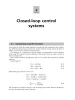
4 CLOSED-LOOP CONTROL SYSTEMS 63
4.1 Closed-loop transfer function 63
4.2 Block diagram reduction 64
4.2.1 Control systems with multiple loops 64
4.2.2 Block diagram manipulation 67
4.3 Systems with multiple inputs 69
4.3.1 Principle of superposition 69
4.4 Transfer functions for system elements 71
4.4.1 DC servo-motors 71
4.4.2 Linear hydraulic actuators 75
4.5 Controllers for closed-loop systems 81
4.5.1 The generalized control problem 81
4.5.2 Proportional control 82

4.5.3 Proportional plus Integral (PI) control 84
vi Contents
//SYS21///SYS21/D/B&H3B2/ACE/REVISES(08-08-01)/ACEA01.3D ± 7 ± [1±14/14] 11.8.2001 12:37PM
4.5.4 Proportional plus Integral plus Derivative (PID) control 89
4.5.5 The Ziegler±Nichols methods for tuning PID controllers 90
4.5.6 Proportional plus Derivative (PD) control 92
4.6 Case study examples 92
4.7 Further problems 104
5 CLASSICAL DESIGN IN THE s-PLANE 110
5.1 Stability of dynamic systems 110
5.1.1 Stability and roots of the characteristic equation 112
5.2 The Routh±Hurwitz stability criterion 112
5.2.1 Maximum value of the open-loop gain constant
for the stability of a closed-loop system 114
5.2.2 Special cases of the Routh array 117
5.3 Root-locus analysis 118
5.3.1 System poles and zeros 118
5.3.2 The root locus method 119
5.3.3 General case for an underdamped second-order system 122
5.3.4 Rules for root locus construction 123
5.3.5 Root locus construction rules 125
5.4 Design in the s-plane 132
5.4.1 Compensator design 133
5.5 Further problems 141
6 CLASSICAL DESIGN IN THE FREQUENCY DOMAIN 145
6.1 Frequency domain analysis 145
6.2 The complex frequency approach 147
6.2.1 Frequency response characteristics of first-order systems 147
6.2.2 Frequency response characteristics of second-order
systems 150

6.3 The Bode diagram 151
6.3.1 Summation of system elements on a Bode diagram 152
6.3.2 Asymptotic approximation on Bode diagrams 153
6.4 Stability in the frequency domain 161
6.4.1 Conformal mapping and Cauchy's theorem 161
6.4.2 The Nyquist stability criterion 162
6.5 Relationship between open-loop and closed-loop frequency response 172
6.5.1 Closed-loop frequency response 172
6.6 Compensator design in the frequency domain 178
6.6.1 Phase lead compensation 179
6.6.2 Phase lag compensation 189
6.7 Relationship between frequency response and time response
for closed-loop systems 191
6.8 Further problems 193
7 DIGITAL CONTROL SYSTEM DESIGN 198
7.1 Microprocessor control 198
7.2 Shannon's sampling theorem 200
Contents vii
//SYS21///SYS21/D/B&H3B2/ACE/REVISES(08-08-01)/ACEA01.3D ± 8 ± [1±14/14] 11.8.2001 12:37PM
7.3 Ideal sampling 201
7.4 The z-transform 202
7.4.1 Inverse transformation 204
7.4.2 The pulse transfer function 206
7.4.3 The closed-loop pulse transfer function 209
7.5 Digital control systems 210
7.6 Stability in the z-plane 213
7.6.1 Mapping from the s-plane into the z-plane 213
7.6.2 The Jury stability test 215
7.6.3 Root locus analysis in the z -plane 218
7.6.4 Root locus construction rules 218

7.7 Digital compensator design 220
7.7.1 Digital compensator types 221
7.7.2 Digital compensator design using pole placement 224
7.8 Further problems 229
8 STATE-SPACE METHODS FOR CONTROL SYSTEM DESIGN 232
8.1 The state-space-approach 232
8.1.1 The concept of state 232
8.1.2 The state vector differential equation 233
8.1.3 State equations from transfer functions 238
8.2 Solution of the state vector differential equation 239
8.2.1 Transient solution from a set of initial conditions 241
8.3 Discrete-time solution of the state vector differential equation 244
8.4 Control of multivariable systems 248
8.4.1 Controllability and observability 248
8.4.2 State variable feedback design 249
8.4.3 State observers 254
8.4.4 Effect of a full-order state observer on a
closed-loop system 260
8.4.5 Reduced-order state observers 262
8.5 Further problems 266
9 OPTIMAL AND ROBUST CONTROL SYSTEM DESIGN 272
9.1 Review of optimal control 272
9.1.1 Types of optimal control problems 272
9.1.2 Selection of performance index 273
9.2 The Linear Quadratic Regulator 274
9.2.1 Continuous form 274
9.2.2 Discrete form 276
9.3 The linear quadratic tracking problem 280
9.3.1 Continuous form 280
9.3.2 Discrete form 281

9.4 The Kalman filter 284
9.4.1 The state estimation process 284
9.4.2 The Kalman filter single variable estimation problem 285
9.4.3 The Kalman filter multivariable state estimation problem 286
viii Contents
//SYS21///SYS21/D/B&H3B2/ACE/REVISES(08-08-01)/ACEA01.3D ± 9 ± [1±14/14] 11.8.2001 12:37PM
9.5 Linear Quadratic Gaussian control system design 288
9.6 Robust control 299
9.6.1 Introduction 299
9.6.2 Classical feedback control 300
9.6.3 Internal Model Control (IMC) 301
9.6.4 IMC performance 302
9.6.5 Structured and unstructured model uncertainty 303
9.6.6 Normalized system inputs 304
9.7 H
2
- and H
I
-optimal control 305
9.7.1 Linear quadratic H
2
-optimal control 305
9.7.2 H
I
-optimal control 306
9.8 Robust stability and robust performance 306
9.8.1 Robust stability 306
9.8.2 Robust performance 308
9.9 Multivariable robust control 314
9.9.1 Plant equations 314

9.9.2 Singular value loop shaping 315
9.9.3 Multivariable H
2
and H
I
robust control 316
9.9.4 The weighted mixed-sensitivity approach 317
9.10 Further problems 321
10 INTELLIGENT CONTROL SYSTEM DESIGN 325
10.1 Intelligent control systems 325
10.1.1 Intelligence in machines 325
10.1.2 Control system structure 325
10.2 Fuzzy logic control systems 326
10.2.1 Fuzzy set theory 326
10.2.2 Basic fuzzy set operations 328
10.2.3 Fuzzy relations 330
10.2.4 Fuzzy logic control 331
10.2.5 Self-organizing fuzzy logic control 344
10.3 Neural network control systems 347
10.3.1 Artificial neural networks 347
10.3.2 Operation of a single artificial neuron 348
10.3.3 Network architecture 349
10.3.4 Learning in neural networks 350
10.3.5 Back-Propagation 351
10.3.6 Application of neural networks to modelling,
estimation and control 358
10.3.7 Neurofuzzy control 361
10.4 Genetic algorithms and their application to control
system design 365
10.4.1 Evolutionary design techniques 365

10.4.2 The genetic algorithm 365
10.4.3. Alternative search strategies 372
10.5 Further problems 373
Contents ix
//SYS21///SYS21/D/B&H3B2/ACE/REVISES(08-08-01)/ACEA01.3D ± 10 ± [1±14/14] 11.8.2001 12:37PM
APPENDIX 1 CONTROL SYSTEM DESIGN USING MATLAB 380
APPENDIX 2 MATRIX ALGEBRA 424
References and further reading 428
Index 433
x Contents
//SYS21///SYS21/D/B&H3B2/ACE/REVISES(08-08-01)/ACEA01.3D ± 11 ± [1±14/14] 11.8.2001 12:37PM
List of Tables
3.1 Common Laplace transform pairs 38
3.2 Unit step response of a first-order system 45
3.3 Unit ramp response of a first-order system 48
3.4 Transient behaviour of a second-order system 50
4.1 Block diagram transformation theorems 67
4.2 Ziegler±Nichols PID parameters using the process reaction method 91
4.3 Ziegler±Nichols PID parameters using the continuous cycling method 91
5.1 Roots of second-order characteristic equation for different values of K 121
5.2 Compensator characteristics 133
6.1 Modulus and phase for a first-order system 149
6.2 Modulus and phase for a second-order system 150
6.3 Data for Nyquist diagram for system in Figure 6.20 167
6.4 Relationship between input function, system type and steady-state error 170
6.5 Open-loop frequency response data 195
7.1 Common Laplace and z-transforms 204
7.2 Comparison between discrete and continuous step response 209
7.3 Comparison between discrete and continuous ramp response 209
7.4 Jury's array 216

9.1 Variations in dryer temperature and moisture content 292
9.2 Robust performance for Example 9.5 313
10.1 Selection of parents for mating from initial population 367
10.2 Fitness of first generation of offsprings 368
10.3 Fitness of second generation of offsprings 368
10.4 Parent selection from initial population for Example 10.6 370
10.5 Fitness of first generation of offsprings for Example 10.6 371
10.6 Fitness of sixth generation of offsprings for Example 10.6 371
10.7 Solution to Example 10.8 376
//SYS21///SYS21/D/B&H3B2/ACE/REVISES(08-08-01)/ACEA01.3D ± 12 ± [1±14/14] 11.8.2001 12:37PM
Preface and
acknowledgements
The material presented in this book is as a result of four decades of experience in the
field of control engineering. During the 1960s, following an engineering apprentice-
ship in the aircraft industry, I worked as a development engineer on flight control
systems for high-speed military aircraft. It was during this period that I first observed
an unstable control system, was shown how to frequency-response test a system and
its elements, and how to plot a Bode and Nyquist diagram. All calculations were
undertaken on a slide-rule, which I still have. Also during this period I worked in
the process industry where I soon discovered that the incorrect tuning for a PID
controller on a 100 m long drying oven could cause catastrophic results.
On the 1st September 1970 I entered academia as a lecturer (Grade II) and in that
first year, as I prepared my lecture notes, I realized just how little I knew about
control engineering. My professional life from that moment on has been one of
discovery (currently termed `life-long learning'). During the 1970s I registered for
an M.Phil. which resulted in writing a FORTRAN program to solve the matrix
Riccati equations and to implement the resulting control algorithm in assembler on a
minicomputer.
In the early 1980s I completed a Ph.D. research investigation into linear quadratic
Gaussian control of large ships in confined waters. For the past 17 years I have

supervised a large number of research and consultancy projects in such areas as
modelling the dynamic behaviour of moving bodies (including ships, aircraft missiles
and weapons release systems) and extracting information using state estimation
techniques from systems with noisy or incomplete data. More recently, research
projects have focused on the application of artificial intelligence techniques to
control engineering projects. One of the main reasons for writing this book has been
to try and capture four decades of experience into one text, in the hope that engineers
of the future benefit from control system design methods developed by engineers of
my generation.
The text of the book is intended to be a comprehensive treatment of control
engineering for any undergraduate course where this appears as a topic. The book
is also intended to be a reference source for practising engineers, students under-
taking Masters degrees, and an introductory text for Ph.D. research students.
//SYS21///SYS21/D/B&H3B2/ACE/REVISES(08-08-01)/ACEA01.3D ± 13 ± [1±14/14] 11.8.2001 12:37PM
One of the fundamental aims in preparing the text has been to work from basic
principles and to present control theory in a way that is easily understood and
applied. For most examples in the book, all that is required to obtain a solution
is a calculator. However, it is recognized that powerful software packages exist to
aid control system design. At the time of writing, MATLAB, its Toolboxes and
SIMULINK have emerged as becoming the industry standard control system design
package. As a result, Appendix 1 provides script file source code for most examples
presented in the main text of the book. It is suggested however, that these script files
be used to check hand calculation when used in a tutorial environment.
Depending upon the structure of the undergraduate programme, it is suggested
that content of Chapters 1, 2 and 3 be delivered in Semester 3 (first Semester, year
two), where, at the same time, Laplace Transforms and complex variables are being
studied under a Mathematics module. Chapters 4, 5 and 6 could then be studied in
Semester 4 (second Semester, year two). In year 3, Chapters 7 and 8 could be studied
in Semester 5 (first Semester) and Chapters 9 and 10 in Semester 6 (second Semester).
However, some of the advanced material in Chapters 9 and 10 could be held back

and delivered as part of a Masters programme.
When compiling the material for the book, decisions had to be made as to what
should be included, and what should not. It was decided to place the emphasis on the
control of continuous and discrete-time linear systems. Treatment of nonlinear
systems (other than linearization) has therefore not been included and it is suggested
that other works (such as Feedback Control Systems, Phillips and Harbor (2000)) be
consulted as necessary.
I would wish to acknowledge the many colleagues, undergraduate and postgrad-
uate students at the University of Plymouth (UoP), University College London
(UCL) and the Open University (OU) who have contributed to the development of
this book. I am especially indebted to the late Professor Tom Lambert (UCL), the
late Professor David Broome (UCL), ex-research students Dr Martyn Polkinghorne,
Dr Paul Craven and Dr Ralph Richter. I would like to thank also my colleague Dr
Bob Sutton, Reader in Control Systems Engineering, in stimulating my interest in the
application of artificial intelligence to control systems design. Thanks also go to OU
students Barry Drew and David Barrett for allowing me to use their T401 project
material in this book. Finally, I would like to express my gratitude to my family. In
particular, I would like to thank Andrew, my son, and Janet my wife, for not only
typing the text of the book and producing the drawings, but also for their complete
support, without which the undertaking would not have been possible.
Roland S. Burns
Preface and acknowledgements xiii
//SYS21///SYS21/D/B&H3B2/ACE/REVISES(08-08-01)/ACEA01.3D ± 14 ± [1±14/14] 11.8.2001 12:37PM
//SYS21/G:/B&H3B2/ACE/REVISES(08-08-01)/ACEC01.3D ± 1 ± [1±12/12] 10.8.2001 3:23PM
1
Introduction to control
engineering
1.1 Historical review
Throughout history mankind has tried to control the world in which he lives. From
the earliest days he realized that his puny strength was no match for the creatures

around him. He could only survive by using his wits and cunning. His major asset
over all other life forms on earth was his superior intelligence. Stone Age man devised
tools and weapons from flint, stone and bone and discovered that it was possible to
train other animals to do his bidding ± and so the earliest form of control system was
conceived. Before long the horse and ox were deployed to undertake a variety of
tasks, including transport. It took a long time before man learned to replace animals
with machines.
Fundamental to any control system is the ability to measure the output of the
system, and to take corrective action if its value deviates from some desired value.
This in turn necessitates a sensing device. Man has a number of `in-built' senses
which from the beginning of time he has used to control his own actions, the actions
of others, and more recently, the actions of machines. In driving a vehicle for
example, the most important sense is sight, but hearing and smell can also contribute
to the driver's actions.
The first major step in machine design, which in turn heralded the industrial
revolution, was the development of the steam engine. A problem that faced engineers
at the time was how to control the speed of rotation of the engine without human
intervention. Of the various methods attempted, the most successful was the use of
a conical pendulum, whose angle of inclination was a function (but not a linear
function) of the angular velocity of the shaft. This principle was employed by James
Watt in 1769 in his design of a flyball, or centrifugal speed governor. Thus possibly
the first system for the automatic control of a machine was born.
The principle of operation of the Watt governor is shown in Figure 1.1, where
change in shaft speed will result in a different conical angle of the flyballs. This in
turn results in linear motion of the sleeve which adjusts the steam mass flow-rate to
the engine by means of a valve.
Watt was a practical engineer and did not have much time for theoretical analysis.
He did, however, observe that under certain conditions the engine appeared to hunt,
//SYS21/G:/B&H3B2/ACE/REVISES(08-08-01)/ACEC01.3D ± 2 ± [1±12/12] 10.8.2001 3:23PM
where the speed output oscillated about its desired value. The elimination of hunting,

or as it is more commonly known, instability, is an important feature in the design of
all control systems.
In his paper `On Governors', Maxwell (1868) developed the differential equations
for a governor, linearized about an equilibrium point, and demonstrated that stabil-
ity of the system depended upon the roots of a characteristic equation having
negative real parts. The problem of identifying stability criteria for linear systems
was studied by Hurwitz (1875) and Routh (1905). This was extended to consider the
stability of nonlinear systems by a Russian mathematician Lyapunov (1893). The
essential mathematical framework for theoretical analysis was developed by Laplace
(1749±1827) and Fourier (1758±1830).
Work on feedback amplifier design at Bell Telephone Laboratories in the 1930s was
based on the concept of frequency response and backed by the mathematics of complex
variables. This was discussed by Nyquist (1932) in his paper `Regeneration Theory',
which described how to determine system stability using frequency domain methods.
This was extended by Bode (1945) and Nichols during the next 15 years to give birth to
what is still one of the most commonly used control system design methodologies.
Another important approach to control system design was developed by Evans
(1948). Based on the work of Maxwell and Routh, Evans, in his Root Locus method,
designed rules and techniques that allowed the roots of the characteristic equation to
be displayed in a graphical manner.
Valve
Steam
Sleeve
Flyballs
Fig. 1.1 The Watt centrifugal speed governor.
2 Advanced Control Engineering
//SYS21/G:/B&H3B2/ACE/REVISES(08-08-01)/ACEC01.3D ± 3 ± [1±12/12] 10.8.2001 3:23PM
The advent of digital computers in the 1950s gave rise to the state-space formula-
tion of differential equations, which, using vector matrix notation, lends itself readily
to machine computation. The idea of optimum design was first mooted by Wiener

(1949). The method of dynamic programming was developed by Bellman (1957), at
about the same time as the maximum principle was discussed by Pontryagin (1962).
At the first conference of the International Federation of Automatic Control
(IFAC), Kalman (1960) introduced the dual concept of controllability and observ-
ability. At the same time Kalman demonstrated that when the system dynamic
equations are linear and the performance criterion is quadratic (LQ control), then
the mathematical problem has an explicit solution which provides an optimal control
law. Also Kalman and Bucy (1961) developed the idea of an optimal filter (Kalman
filter) which, when combined with an optimal controller, produced linear-quadratic-
Gaussian (LQG) control.
The 1980s saw great advances in control theory for the robust design of systems
with uncertainties in their dynamic characteristics. The work of Athans (1971),
Safanov (1980), Chiang (1988), Grimble (1988) and others demonstrated how uncer-
tainty can be modelled and the concept of the HI norm and -synthesis theory.
The 1990s has introduced to the control community the concept of intelligent
control systems. An intelligent machine according to Rzevski (1995) is one that is
able to achieve a goal or sustained behaviour under conditions of uncertainty.
Intelligent control theory owes much of its roots to ideas laid down in the field of
Artificial Intelligence (AI). Artificial Neural Networks (ANNs) are composed of
many simple computing elements operating in parallel in an attempt to emulate their
biological counterparts. The theory is based on work undertaken by Hebb (1949),
Rosenblatt (1961), Kohonen (1987), Widrow-Hoff (1960) and others. The concept of
fuzzy logic was introduced by Zadeh (1965). This new logic was developed to allow
computers to model human vagueness. Fuzzy logic controllers, whilst lacking the
formal rigorous design methodology of other techniques, offer robust control with-
out the need to model the dynamic behaviour of the system. Workers in the field
include Mamdani (1976), Sugeno (1985) Sutton (1991) and Tong (1978).
1.2 Control system fundamentals
1.2.1 Concept of a system
Before discussing the structure of a control system it is necessary to define what is

meant by a system. Systems mean different things to different people and can include
purely physical systems such as the machine table of a Computer Numerically
Controlled (CNC) machine tool or alternatively the procedures necessary for the
purchase of raw materials together with the control of inventory in a Material
Requirements Planning (MRP) system.
However, all systems have certain things in common. They all, for example,
require inputs and outputs to be specified. In the case of the CNC machine tool
machine table, the input might be the power to the drive motor, and the outputs
might be the position, velocity and acceleration of the table. For the MRP system
inputs would include sales orders and sales forecasts (incorporated in a master
Introduction to control engineering 3
//SYS21/G:/B&H3B2/ACE/REVISES(08-08-01)/ACEC01.3D ± 4 ± [1±12/12] 10.8.2001 3:23PM
production schedule), a bill of materials for component parts and subassemblies,
inventory records and information relating to capacity requirements planning. Mate-
rial requirements planning systems generate various output reports that are used in
planning and managing factory operations. These include order releases, inventory
status, overdue orders and inventory forecasts. It is necessary to clearly define the
boundary of a system, together with the inputs and outputs that cross that boundary.
In general, a system may be defined as a collection of matter, parts, components or
procedures which are included within some specified boundary as shown in Figure
1.2. A system may have any number of inputs and outputs.
In control engineering, the way in which the system outputs respond in changes to
the system inputs (i.e. the system response) is very important. The control system
design engineer will attempt to evaluate the system response by determining a
mathematical model for the system. Knowledge of the system inputs, together with
the mathematical model, will allow the system outputs to be calculated.
It is conventional to refer to the system being controlled as the plant, and this, as
with other elements, is represented by a block diagram. Some inputs, the engineer will
have direct control over, and can be used to control the plant outputs. These are
known as control inputs. There are other inputs over which the engineer has no

control, and these will tend to deflect the plant outputs from their desired values.
These are called disturbance inputs.
In the case of the ship shown in Figure 1.3, the rudder and engines are the control
inputs, whose values can be adjusted to control certain outputs, for example heading
and forward velocity. The wind, waves and current are disturbance inputs and will
induce errors in the outputs (called controlled variables) of position, heading and
forward velocity. In addition, the disturbances will introduce increased ship motion
(roll, pitch and heave) which again is not desirable.
System
Boundary
Inputs
Outputs
Fig. 1.2 The concept of a system.
Rudder
Position
Engines
Forward Velocity
Velocity
Wind
Heading
Waves
Ship Motion
(roll, pitch, heave)
Current
Ship
Fig. 1.3 Ashipasadynamicsystem.
4 Advanced Control Engineering
//SYS21/G:/B&H3B2/ACE/REVISES(08-08-01)/ACEC01.3D ± 5 ± [1±12/12] 10.8.2001 3:23PM
Generally, the relationship between control input, disturbance input, plant and
controlled variable is shown in Figure 1.4.

1.2.2 Open-loop systems
Figure 1.4 represents an open-loop control system and is used for very simple
applications. The main problem with open-loop control is that the controlled vari-
able is sensitive to changes in disturbance inputs. So, for example, if a gas fire is
switched on in a room, and the temperature climbs to 20

C, it will remain at that
value unless there is a disturbance. This could be caused by leaving a door to the
room open, for example. Or alternatively by a change in outside temperature. In
either case, the internal room temperature will change. For the room temperature to
remain constant, a mechanism is required to vary the energy output from the gas fire.
1.2.3 Closed-loop systems
For a room temperature control system, the first requirement is to detect or sense
changes in room temperature. The second requirement is to control or vary the energy
output from the gas fire, if the sensed room temperature is different from the desired
room temperature. In general, a system that is designed to control the output of a
plant must contain at least one sensor and controller as shown in Figure 1.5.
Disturbance
Input
Control Input
Controlled Variable
or
Output
+
Summing
Point
Plant
–
Fig. 1.4 Plant inputs and outputs.
Forward Path

Controller
Control
Signal
Summing
Point
Error
Signal
Output
Value
•
Measured Value
Feedback Path
Desired Value
Plant
Sensor
+
–
Fig. 1.5 Closed-loop control system.
Introduction to control engineering 5
//SYS21/G:/B&H3B2/ACE/REVISES(08-08-01)/ACEC01.3D ± 6 ± [1±12/12] 10.8.2001 3:23PM
Figure 1.5 shows the generalized schematic block-diagram for a closed-loop, or
feedback control system. The controller and plant lie along the forward path, and the
sensor in the feedback path. The measured value of the plant output is compared at
the summing point with the desired value. The difference, or error is fed to the
controller which generates a control signal to drive the plant until its output equals
the desired value. Such an arrangement is sometimes called an error-actuated system.
1.3 Examples of control systems
1.3.1 Room temperature control system
The physical realization of a system to control room temperature is shown in Figure
1.6. Here the output signal from a temperature sensing device such as a thermocouple

or a resistance thermometer is compared with the desired temperature. Any differ-
ence or error causes the controller to send a control signal to the gas solenoid valve
which produces a linear movement of the valve stem, thus adjusting the flow of gas to
the burner of the gas fire. The desired temperature is usually obtained from manual
adjustment of a potentiometer.
Desired
Temperature
Measured
Temperature
Potentio-
meter
Controller
Control
Signal
Gas Solenoid
Valve
Outside
Temperature
Heat
Loss
Insulation
Actual
Room
Temperature
Gas
Fire
Heat
Input
Thermometer
Gas

Flow-rate
Fig. 1.6 Room temperature control system.
Desired
Temperature
Potentio-
meter
(°C)
Error
Signal
Control
Signal
Controller
+
(V)
–
(V) (V)
Gas
Solenoid
Valve
Gas
Burner
Room
Insula-
tion
Gas
Flow-rate
(m /s)
3
Thermometer
(V)

Outside
Temperature
Actual
Temperature
(°C)
+
Heat
Input
(W)
Heat
Loss
(W)
–
Fig. 1.7 Block diagram of room temperature control system.
6 Advanced Control Engineering
//SYS21/G:/B&H3B2/ACE/REVISES(08-08-01)/ACEC01.3D ± 7 ± [1±12/12] 10.8.2001 3:23PM
A detailed block diagram is shown in Figure 1.7. The physical values of the signals
around the control loop are shown in brackets.
Steady conditions will exist when the actual and desired temperatures are the same,
and the heat input exactly balances the heat loss through the walls of the building.
The system can operate in two modes:
(a) Proportional control: Here the linear movement of the valve stem is proportional to
the error. This provides a continuous modulation of the heat input to the room
producing very precise temperature control. This is used for applications where temp-
erature control, of say better than 1

C, is required (i.e. hospital operating theatres,
industrial standards rooms, etc.) where accuracy is more important than cost.
(b) On±off control: Also called thermostatic or bang-bang control, the gas valve is
either fully open or fully closed, i.e. the heater is either on or off. This form of

control produces an oscillation of about 2 or 3

C of the actual temperature
about the desired temperature, but is cheap to implement and is used for low-cost
applications (i.e. domestic heating systems).
1.3.2 Aircraft elevator control
In the early days of flight, control surfaces of aircraft were operated by cables
connected between the control column and the elevators and ailerons. Modern
high-speed aircraft require power-assisted devices, or servomechanisms to provide
the large forces necessary to operate the control surfaces.
Figure 1.8 shows an elevator control system for a high-speed jet.
Movement of the control column produces a signal from the input angular sensor
which is compared with the measured elevator angle by the controller which generates
a control signal proportional to the error. This is fed to an electrohydraulic servovalve
which generates a spool-valve movement that is proportional to the control signal,
Desired
Angle
Desired
Angle
Control
Column
Control
Column
Actual
Angle
Actual
Angle
Measured AngleMeasured Angle
Control Signal
ControllerController

ElevatorElevator
Output Angular
Sensor
Output Angular
Sensor
Hydraulic
Cylinder
Hydraulic
Cylinder
Electrohydraulic
Servovalve
Input
Angular
Sensor
Fig. 1.8 Elevator control system for a high-speed jet.
Introduction to control engineering 7
//SYS21/G:/B&H3B2/ACE/REVISES(08-08-01)/ACEC01.3D ± 8 ± [1±12/12] 10.8.2001 3:23PM
thus allowing high-pressure fluid to enter the hydraulic cylinder. The pressure differ-
ence across the piston provides the actuating force to operate the elevator.
Hydraulic servomechanisms have a good power/weight ratio, and are ideal for
applications that require large forces to be produced by small and light devices.
In practice, a `feel simulator' is attached to the control column to allow the pilot to
sense the magnitude of the aerodynamic forces acting on the control surfaces, thus
preventing excess loading of the wings and tail-plane. The block diagram for the
elevator control system is shown in Figure 1.9.
1.3.3 Computer Numerically Controlled (CNC) machine tool
Many systems operate under computer control, and Figure 1.10 shows an example of
a CNC machine tool control system.
Information relating to the shape of the work-piece and hence the motion of the
machine table is stored in a computer program. This is relayed in digital format, in a

sequential form to the controller and is compared with a digital feedback signal from
the shaft encoder to generate a digital error signal. This is converted to an analogue
Desired
Angle
(deg)
Input
Angular
Sensor
Error
Signal
Controller
Servo-
valve
Hydraulic
Cylinder
Elevator
Hydraulic
Force
(N)
Actual
Angle
(deg)
Control
Signal
Output
Angular
Sensor
Fluid
Flow-rate
(m /s)

3
(V)
(V)
(V)
(V)
+
–
Fig. 1.9 Block diagram of elevator control system.
Computer
Controller
Machine Table Movement
Computer
Program
Digital
Controller
Power
Amplifier
Lead-Screw
Digital Positional Feedback
Analogue Velocity Feedback
Bearing
Tachogenerato
r
Shaft
Encoder
DC-Servomotor
Fig. 1.10 Computer numerically controlled machine tool.
8 Advanced Control Engineering
//SYS21/G:/B&H3B2/ACE/REVISES(08-08-01)/ACEC01.3D ± 9 ± [1±12/12] 10.8.2001 3:23PM
control signal which, when amplified, drives a d.c. servomotor. Connected to the

output shaft of the servomotor (in some cases through a gearbox) is a lead-screw to
which is attached the machine table, the shaft encoder and a tachogenerator. The
purpose of this latter device, which produces an analogue signal proportional to
velocity, is to form an inner, or minor control loop in order to dampen, or stabilize
the response of the system.
The block diagram for the CNC machine tool control system is shown in Figure 1.11.
1.3.4 Ship autopilot control system
A ship autopilot is designed to maintain a vessel on a set heading while being
subjected to a series of disturbances such as wind, waves and current as shown in
Figure 1.3. This method of control is referred to as course-keeping. The autopilot can
also be used to change course to a new heading, called course-changing. The main
elements of the autopilot system are shown in Figure 1.12.
The actual heading is measured by a gyro-compass (or magnetic compass in a
smaller vessel), and compared with the desired heading, dialled into the autopilot by
the ship's master. The autopilot, or controller, computes the demanded rudder angle
and sends a control signal to the steering gear. The actual rudder angle is monitored
by a rudder angle sensor and compared with the demanded rudder angle, to form a
control loop not dissimilar to the elevator control system shown in Figure 1.8.
The rudder provides a control moment on the hull to drive the actual heading
towards the desired heading while the wind, waves and current produce moments that
may help or hinder this action. The block diagram of the system is shown in Figure 1.13.
Digital
Desired Position
Digital
Error
Computer
Program
Digital
Controller
Power

Amplifier
+
(V)
Control
Signal
(V)
DC
Servo
motor
Torque
(Nm)
Actual
Velocity
(m/s)
Machine
Ta bl e
Actual
Position
(m)
Integrator
Analogue
Tacho-
generator
Velocity Feedback
Shaft
Encoder
Digital Positional
Feedback
+
–

–
Fig. 1.11 Block diagram of CNC machine-tool control system.
Desired Heading
Actual rudder-angle
Gyro-compass
Error
Actual Heading
Auto-pilot
Demanded rudder-angle
Measured rudder-angle
Steering-gear
Sensor
Fig. 1.12 Ship autopilot control system.
Introduction to control engineering 9
//SYS21/G:/B&H3B2/ACE/REVISES(08-08-01)/ACEC01.3D ± 10 ± [1±12/12] 10.8.2001 3:23PM
1.4 Summary
In order to design and implement a control system the following essential generic
elements are required:
.
Knowledge of the desired value: It is necessary to know what it is you are trying to
control, to what accuracy, and over what range of values. This must be expressed
in the form of a performance specification. In the physical system this information
must be converted into a form suitable for the controller to understand (analogue
or digital signal).
.
Knowledge of the output or actual value: This must be measured by a feedback
sensor, again in a form suitable for the controller to understand. In addition, the
sensor must have the necessary resolution and dynamic response so that the
measured value has the accuracy required from the performance specification.
.

Knowledge of the controlling device: The controller must be able to accept meas-
urements of desired and actual values and compute a control signal in a suitable
form to drive an actuating element. Controllers can be a range of devices, including
mechanical levers, pneumatic elements, analogue or digital circuits or microcomputers.
.
Knowledge of the actuating device: This unit amplifies the control signal and
provides the `effort' to move the output of the plant towards its desired value. In
the case of the room temperature control system the actuator is the gas solenoid valve
and burner, the `effort' being heat input (W). For the ship autopilot system the
actuator is the steering gear and rudder, the `effort' being turning moment (Nm).
.
Knowledge of the plant: Most control strategies require some knowledge of the
static and dynamic characteristics of the plant. These can be obtained from
measurements or from the application of fundamental physical laws, or a com-
bination of both.
1.4.1 Control system design
With all of this knowledge and information available to the control system designer,
all that is left is to design the system. The first problem to be encountered is that the
Desired
Heading
(deg)
Potentio-
meter
Autopilot
(Controller)
Course
Error
(V)
(V)
–

+
Measured
Heading (V)
Steering
Gear
Rudder
Charact-
eristics
Hull
Actual
Heading
(deg)
Disturbance
Moment
(Nm)
+ –
Actual
Rudder
Angle
(deg)
Demanded
Rudder
Angle
+
(V)
–
Rudder
Angle
Sensor
Rudder

Moment
(Nm)
Gyro-
Compass
Fig. 1.13 Block diagram of ship autopilot control system.
10 Advanced Control Engineering
//SYS21/G:/B&H3B2/ACE/REVISES(08-08-01)/ACEC01.3D ± 11 ± [1±12/12] 10.8.2001 3:23PM
•
•
•
Define System
Performance
Specification
Is Component
Response Acceptable?
Does Simulated
Response Meet
Performance Specification?
Model Behaviour
of Plant and
System
Components
Identify System
Components
Select
Alternative
Components
Ye s
No
Define Control

Strategy
Simulate
System
Response
Modify
Control
Strategy
Implement
Physical System
Measure System
Response
Modify Control
Strategy
Does System
Response Meet
Performance Specification?
START
Ye s
No
FINISH
No
Ye s
Fig. 1.14 Steps in the design of a control system.
Introduction to control engineering 11
//SYS21/G:/B&H3B2/ACE/REVISES(08-08-01)/ACEC01.3D ± 12 ± [1±12/12] 10.8.2001 3:23PM
knowledge of the system will be uncertain and incomplete. In particular, the dynamic
characteristics of the system may change with time (time-variant) and so a fixed
control strategy will not work. Due to fuel consumption for example, the mass of an
airliner can be almost half that of its take-off value at the end of a long haul flight.
Measurements of the controlled variables will be contaminated with electrical

noise and disturbance effects. Some sensors will provide accurate and reliable data,
others, because of difficulties in measuring the output variable may produce highly
random and almost irrelevant information.
However, there is a standard methodology that can be applied to the design of
most control systems. The steps in this methodology are shown in Figure 1.14.
The design of a control system is a mixture of technique and experience. This book
explains some tried and tested, and some more recent approaches, techniques and
methods available to the control system designer. Experience, however, only comes
with time.
12 Advanced Control Engineering