ț Product category by region by month
ț Product department by region by month
ț All products by region by month
ț Product category by all stores by month
ț Product department by all stores by month
ț Product category by territory by quarter
ț Product department by territory by quarter
ț All products by territory by quarter
ț Product category by region by quarter
ț Product department by region by quarter
ț All products by region by quarter
ț Product category by all stores by quarter
ț Product department by all stores by quarter
ț Product category by territory by year
ț Product department by territory by year
ț All products by territory by year
ț Product category by region by year
ț Product department by region by year
ț All products by region by year
ț Product category by all stores by year
ț Product department by all stores by year
ț All products by all stores by year
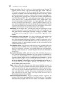
Each of these aggregate fact tables is derived from a single base fact table. The derived
aggregate fact tables are joined to one or more derived dimension tables. See Figure 11-15
showing a derived aggregate fact table connected to a derived dimension table.
Effect of Sparsity on Aggregation. Consider the case of the grocery chain with 300
stores, 40,000 products in each store, but only 4000 selling in each store in a day. As dis-
cussed earlier, assuming that you keep records for 5 years or 1825 days, the maximum
number of base fact table rows is calculated as follows:
Product = 40,000
Store = 300

Time = 1825
Maximum number of base fact table rows = 22 billion
Because only 4,000 products sell in each store in a day, not all of these 22 billion rows
are occupied. Because of this sparsity, only 10% of the rows are occupied. Therefore, the
real estimate of the number of base table rows is 2 billion.
Now let us see what happens when you form aggregates. Scrutinize a one-way aggre-
gate: brand totals by store by day. Calculate the maximum number of rows in this one-way
aggregate.
246
DIMENSIONAL MODELING: ADVANCED TOPICS
Brand = 80
Store = 300
Time = 1825
Maximum number of aggregate table rows = 43,800,000
While creating the one-way aggregate, you will notice that the sparsity for this aggre-
gate is not 10% as in the case of the base table. This is because when you aggregate by
brand, more of the brand codes will participate in combinations with store and time codes.
The sparsity of the one-way aggregate would be about 50%, resulting in a real estimate of
21,900,000. If the sparsity had remained as the 10% applicable to the base table, the real
estimate of the number of rows in the aggregate table would be much less.
When you go for higher levels of aggregates, the sparsity percentage moves up and
even reaches 100%. Because of the failure of sparsity to stay lower, you are faced with the
question whether aggregates do improve performance that much. Do they reduce the
number of rows that dramatically?
Experienced data warehousing practitioners have a suggestion. When you form aggre-
gates, make sure that each aggregate table row summarizes at least 10 rows in the lower
level table. If you increase this to 20 rows or more, it would be really remarkable.
Aggregation Options
Going back to our discussion of one-way, two-way, and three-way aggregates for a basic
STAR schema with just three dimensions, you could count more than 50 different ways you

AGGREGATE FACT TABLES
247
Product Key
Time Key
Store Key
Unit Sales
Sales Dollars
SALES FACTS
STORE
PRODUCT
TIME
Store Key
Store Name
Territory
Region
Time Key
Date
Month
Quarter
Year
Product Key
Product
Category
Department
CATEGORY
Category Key
Category
Department
Category Key
Time Key

Store Key
Unit Sales
Sales Dollars
SALES FACTS
BASE TABLE
ONE-WAY AGGREGATE
DIMENSION
DERIVED FROM
PRODUCT
Figure 11-15 Aggregate fact table and derived dimension table.
may create aggregates. In the real world, the number of dimensions is not just three, but
many more. Therefore, the number of possible aggregate tables escalates into the hundreds.
Further, from the reference to the failure of sparsity in aggregate tables, you know that
the aggregation process does not reduce the number of rows proportionally. In other
words, if the sparsity of the base fact table is 10%, the sparsity of the higher-level aggre-
gate tables does not remain at 10%. The sparsity percentage increases more and more as
your aggregate tables climb higher and higher in levels of summarization.
Is aggregation that much effective after all? What are some of the options? How do you
decide what to aggregate? First, set a few goals for aggregation for your data warehouse
environment.
Goals for Aggregation Strategy. Apart from the general overall goal of improving
data warehouse performance, here are a few specific, practical goals:
ț Do not get bogged down with too many aggregates. Remember, you have to create
additional derived dimensions as well to support the aggregates.
ț Try to cater to a wide range of user groups. In any case, provide for your power
users.
ț Go for aggregates that do not unduly increase the overall usage of storage. Look
carefully into larger aggregates with low sparsity percentages.
ț Keep the aggregates hidden from the end-users. That is, the aggregates must be
transparent to the end-user query. The query tool must be the one to be aware of the

aggregates to direct the queries for proper access.
ț Attempt to keep the impact on the data staging process as less intensive as possible.
Practical Suggestions. Before doing any calculations to determine the types of ag-
gregates needed for your data warehouse environment, spend a good deal of time on de-
termining the nature of the common queries. How do your users normally report results?
What are the reporting levels? By stores? By months? By product categories? Go through
the dimensions, one by one, and review the levels of the hierarchies. Check if there are
multiple hierarchies within the same dimension. If so, find out which of these multiple hi-
erarchies are more important. In each dimension, ascertain which attributes are used for
grouping the fact table metrics. The next step is to determine which of these attributes are
used in combinations and what the most common combinations are.
Once you determine the attributes and their possible combinations, look at the number
of values for each attribute. For example, in a hotel chain schema, assume that hotel is at
the lowest level and city is at the next higher level in the hotel dimension. Let us say there
are 25,000 values for hotel and 15,000 values for city. Clearly, there is no big advantage of
aggregating by cities. On the other hand, if city has only 500 values, then city is a level at
which you may consider aggregation. Examine each attribute in the hierarchies within a
dimension. Check the values for each of the attributes. Compare the values of attributes at
different levels of the same hierarchy and decide which ones are strong candidates to par-
ticipate in aggregation.
Develop a list of attributes that are useful candidates for aggregation, then work out the
combinations of these attributes to come up with your first set of multiway aggregate fact
tables. Determine the derived dimension tables you need to support these aggregate fact
tables. Go ahead and implement these aggregate fact tables as the initial set.
248
DIMENSIONAL MODELING: ADVANCED TOPICS
Bear in mind that aggregation is a performance tuning mechanism. Improved query per-
formance drives the need to summarize, so do not be too concerned if your first set of ag-
gregate tables do not perform perfectly. Your aggregates are meant to be monitored and re-
vised as necessary. The nature of the bulk of the query requests is likely to change. As your

users become more adept at using the data warehouse, they will devise new ways of group-
ing and analyzing data. So what is the practical advice? Do your preparatory work, start
with a reasonable set of aggregate tables, and continue to make adjustments as necessary.
FAMILIES OF STARS
When you look at a single STAR schema with its fact table and the surrounding dimen-
sion tables, you know that is not the extent of a data warehouse. Almost all data warehous-
es contain multiple STAR schema structures. Each STAR serves a specific purpose to
track the measures stored in the fact table. When you have a collection of related STAR
schemas, you may call the collection a family of STARS. Families of STARS are formed
for various reasons. You may form a family by just adding aggregate fact tables and the
derived dimension tables to support the aggregates. Sometimes, you may create a core
fact table containing facts interesting to most users and customized fact tables for specific
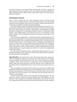
user groups. Many factors lead to the existence of families of STARS. First, look at the
example provided in Figure 11-16.
The fact tables of the STARS in a family share dimension tables. Usually, the time di-
mension is shared by most of the fact tables in the group. In the above example, all the
FAMILIES OF STARS
249
Figure 11-16 Family of STARS.
FACT
TABLE
DIMENSION
TABLE
DIMENSION
TABLE
DIMENSION
TABLE
DIMENSION
TABLE
DIMENSION

TABLE
DIMENSION
TABLE
FACT
TABLE
FACT
TABLE
DIMENSION
TABLE
DIMENSION
TABLE
three fact tables are likely to share the time dimension. Going the other way, dimension ta-
bles from multiple STARS may share the fact table of one STAR.
If you are in a business like banking or telephone services, it makes sense to capture in-
dividual transactions as well as snapshots at specific intervals. You may then use families
of STARS consisting of transaction and snapshot schemas. If you are in a manufacturing
company or a similar production-type enterprise, your company needs to monitor the met-
rics along the value chain. Some other institutions are like a medical center, where value is
added not in a chain but at different stations within the enterprise. For these enterprises,
the family of STARS supports the value chain or the value circle. We will get into details
in the next few sections.
Snapshot and Transaction Tables
Let us review some basic requirements of a telephone company. A number of individual
transactions make up a telephone customer’s account. Many of the transactions occur dur-
ing the hours of 6 a.m. to 10 p.m. of the customer’s day. More transactions happen during
the holidays and weekends for residential customers. Institutional customers use the
phones on weekdays rather than over the weekends. A telephone accumulates a very large
collection of rich transaction data that can be used for many types of valuable analysis.
The telephone company needs a schema capturing transaction data that supports strategic
decision making for expansions, new service improvements, and so on. This transaction

schema answers questions such as how does the revenue of peak hours over the weekends
and holidays compare with peak hours over weekdays.
In addition, the telephone company needs to answer questions from the customers as to
account balances. The customer service departments are constantly bombarded with ques-
tions on the status of individual customer accounts. At periodic intervals, the accounting
department may be interested in the amounts expected to be received by the middle of
next month. What are the outstanding balances for which bills will be sent this month-
end? For these purposes, the telephone company needs a schema to capture snapshots at
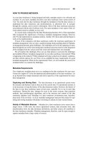
periodic intervals. Please see Figure 11-17 showing the snapshot and transaction fact ta-
bles for a telephone company. Make a note of the attributes in the two fact tables. One
table tracks the individual phone transactions. The other table holds snapshots of individ-
ual accounts at specific intervals. Also, notice how dimension tables are shared between
the two fact tables.
Snapshot and transaction tables are also common for banks. For example, an ATM
transaction table stores individual ATM transactions. This fact table keeps track of indi-
vidual transaction amounts for the customer accounts. The snapshot table holds the bal-
ance for each account at the end of each day. The two tables serve two distinct functions.
From the transaction table, you can perform various types of analysis of the ATM transac-
tions. The snapshot table provides total amounts held at periodic intervals showing the
shifting and movement of balances.
Financial data warehouses also require snapshot and transaction tables because of the
nature of the analysis in these cases. The first set of questions for these warehouses relates
to the transactions affecting given accounts over a certain period of time. The other set of
questions centers around balances in individual accounts at specific intervals or totals of
groups of accounts at the end of specific periods. The transaction table answers the ques-
tions of the first set; the snapshot table handles the questions of the second set.
250
DIMENSIONAL MODELING: ADVANCED TOPICS
Core and Custom Tables
Consider two types of businesses that are apparently dissimilar. First take the case of a

bank. A bank offers a large variety of services all related to finance in one form or anoth-
er. Most of the services are different from one another. The checking account service and
the savings account service are similar in most ways. But the savings account service does
not resemble the credit card service in any way. How do you track these dissimilar ser-
vices?
Next, consider a manufacturing company producing a number of heterogeneous prod-
ucts. Although a few factors may be common to the various products, by and large the fac-
tors differ. What must you do to get information about heterogeneous products?
A different type of the family of STARS satisfies the requirements of these companies.
In this type of family, all products and services connect to a core fact table and each prod-
uct or service relates to individual custom tables. In Figure 11-18, you will see the core
and custom tables for a bank. Note how the core fact table holds the metrics that are com-
mon to all types of accounts. Each custom fact table contains the metrics specific to that
line of service. Also note the shared dimension and notice how the tables form a family of
STARS.
Supporting Enterprise Value Chain or Value Circle
In a manufacturing business, a product travels through various steps, starting off as raw
materials and ending as finished goods in the warehouse inventory. Usually, the steps in-
clude addition of ingredients, assembly of materials, process control, packaging, and ship-
ping to the warehouse. From finished goods inventory, a product moves into shipment to
distributor, distributor inventory, distributor shipment, retail inventory, and retail sales. At
FAMILIES OF STARS
251
Time Key
Account Key
Transaction Key
District Key
Trans Reference
Account Number
Amount

TELEPHONE
TRANSACTION
FACT TABLE
STATUS
Status Key
…………
ACCOUNT
Account Key
…………
DISTRICT
District Key
…………
TIME
Time Key
…………
Time Key
Account Key
Status Key
Transaction Count
Ending Balance
TELEPHONE
SNAPSHOT
FACT TABLE
TRANSACTION
Transaction Key
…………
Figure 11-17 Snapshot and transaction tables.
each step, value is added to the product. Several operational systems support the flow
through these steps. The whole flow forms the supply chain or the value chain. Similarly,
in an insurance company, the value chain may include a number of steps from sales of in-

surance through issuance of policy and then finally claims processing. In this case, the
value chain relates to the service.
If you are in one of these businesses, you need to track important metrics at different
steps along the value chain. You create STAR schemas for the significant steps and the
complete set of related schemas forms a family of STARS. You define a fact table and a
set of corresponding dimensions for each important step in the chain. If your company has
multiple value chains, then you have to support each chain with a separate family of
STARS.
A supply chain or a value chain runs in a linear fashion beginning with a certain step
and ending at another step with many steps in between. Again, at each step, value is
added. In some other kinds of businesses where value gets added to services, similar lin-
ear movements do not exist. For example, consider a health care institution where value
gets added to patient service from different units almost as if they form a circle around the
service. We perceive a value circle in such organizations. The value circle of a large health
maintenance organization may include hospitals, clinics, doctors’ offices, pharmacies,
laboratories, government agencies, and insurance companies. Each of these units either
provide patient treatments or measure patient treatments. Patient treatment by each unit
may be measured in different metrics. But most of the units would analyze the metrics us-
252
DIMENSIONAL MODELING: ADVANCED TOPICS
Time Key
Account Key
Branch Key
Household Key
Balance
Fees Charged
Transactions
BRANCH
Branch Key
…………

ACCOUNT
Account Key
…………
TIME
Time Key
…………
Account Key
Deposits
Withdrawals
Interest Earned
Balance
Service Charges
HOUSEHOLD
Household Key
…………
Account Key
ATM Trans.
Drive-up Trans.
Walk-in Trans.
Deposits
Checks Paid
Overdraft
BANK CORE FACT TABLE
SAVINGS CUSTOM
FACT TABLE
CHECKING CUSTOM
FACT TABLE
Figure 11-18 Core and custom tables.
ing the same set of conformed dimensions such as time, patient, health care provider,
treatment, diagnosis, and payer. For a value circle, the family of STARS comprises multi-

ple fact tables and a set of conformed dimensions.
Conforming Dimensions
While exploring families of STARS, you will have noticed that dimensions are shared
among fact tables. Dimensions form common links between STARS. For dimensions to
be conformed, you have to deliberately make sure that common dimensions may be used
between two or more STARS. If the product dimension is shared between two fact tables
of sales and inventory, then the attributes of the product dimension must have the same
meaning in relation to each of the two fact tables. Figure 11-19 shows a set of conformed
dimensions.
The order and shipment fact tables share the conformed dimensions of product, date,
customer, and salesperson. A conformed dimension is a comprehensive combination of
attributes from the source systems after resolving all discrepancies and conflicts. For ex-
ample, a conformed product dimension must truly reflect the master product list of the en-
terprise and must include all possible hierarchies. Each attribute must be of the correct
data type and must have proper lengths and constraints.
Conforming dimensions is a basic requirement in a data warehouse. Pay special atten-
tion and take the necessary steps to conform all your dimensions. This is a major respon-
sibility of the project team. Conformed dimensions allow rollups across data marts. User
interfaces will be consistent irrespective of the type of query. Result sets of queries will be
FAMILIES OF STARS
253
Product Key
Time Key
Customer Key
Salesperson Key
Order Dollars
Cost Dollars
Margin Dollars
Sale Units
ORDER

CUSTOMER
SALESPERSON
PRODUCT
DATE
Customer Key
……………….
Salesperson Key
………………
Date Key
………………
Product Key
……………
Product Key
Time Key
Customer Key
Salesperson Key
Channel Key
Ship-to Key
Ship-from Key
Invoice Number
Order Number
Ship Date
Arrival Date
SHIPMENT
CHANNEL
Channel Key
………………
SHIP-TO
Ship-to Key
………………

SHIP-FROM
Ship-from Key
………………
CONFORMED
DIMENSIONS
Figure 11-19 Conformed dimensions.
consistent across data marts. Of course, a single conformed dimension can be used
against multiple fact tables.
Standardizing Facts
In addition to the task of conforming dimensions is the requirement to standardize facts.
We have seen that fact tables work across STAR schemas. Review the following issues re-
lating to the standardization of fact table attributes:
ț Ensure same definitions and terminology across data marts
ț Resolve homonyms and synonyms
ț Types of facts to be standardized include revenue, price, cost, and profit margin
ț Guarantee that the same algorithms are used for any derived units in each fact
table
ț Make sure each fact uses the right unit of measurement
Summary of Family of STARS
Let us end our discussion of the family of STARS with a comprehensive diagram showing
a set of standardized fact tables and conformed dimension tables. Study Figure 11-20 care-
254
DIMENSIONAL MODELING: ADVANCED TOPICS
Date Key
Account Key
Branch Key
Balance
BRANCH
Branch Key
Branch Name

State
Region
ACCOUNT
Account Key
…………
DATE
Date Key
Date
Month
Year
Account Key
ATM Trans.
Other Trans.
STATE
State Key
State
Region
Date Key
Account Kye
State Key
Balance
MONTH
Month Key
Month
Year
Month Key
Account Key
State Key
Balance
2-WAY AGGREGATE

1-WAY AGGREGATE
BANK CORE TABLE
CHECKING CUSTOM TABLE
Figure 11-20 A comprehensive family of STARS.
Branch Name
fully. Note the aggregate fact tables and the corresponding derived dimension tables. What
types of aggregates are these? One-way or two-way? Which are the base fact tables? Notice
the shared dimensions. Are these conformed dimensions? See how the various fact tables
and the dimension tables are related.
CHAPTER SUMMARY
ț Slowly changing dimensions may be classified into three different types based on
the nature of the changes. Type 1 relates to corrections, Type 2 to preservation of
history, and Type 3 to soft revisions. Applying each type of revision to the data
warehouse is different.
ț Large dimension tables such as customer or product need special considerations for
applying optimizing techniques.
ț “Snowflaking” or creating a snowflake schema is a method of normalizing the
STAR schema. Although some conditions justify the snowflake schema, it is gener-
ally not recommended.
ț Miscellaneous flags and textual data are thrown together in one table called a junk
dimension table.
ț Aggregate or summary tables improve performance. Formulate a strategy for build-
ing aggregate tables.
ț A set of related STAR schemas make up a family of STARS. Examples are snapshot
and transaction tables, core and custom tables, and tables supporting a value chain
or a value circle. A family of STARS relies on conformed dimension tables and
standardized fact tables.
REVIEW QUESTIONS
1. Describe slowly changing dimensions. What are the three types? Explain each
type very briefly.

2. Compare and contrast Type 2 and Type 3 slowly changing dimensions.
3. Can you treat rapidly changing dimensions in the same way as Type 2 slowly
changing dimensions? Discuss.
4. What are junk dimensions? Are they necessary in a data warehouse?
5. How does a snowflake schema differ from a STAR schema? Name two advantages
and two disadvantages of the snowflake schema.
6. Differentiate between slowly and rapidly changing dimensions.
7. What are aggregate fact tables? Why are they needed? Give an example.
8. Describe with examples snapshot and transaction fact tables. How are they relat-
ed?
9. Give an example of a value circle. Explain how a family of STARS can support a
value circle.
10. What is meant by conforming the dimensions? Why is this important in a data
warehouse?
REVIEW QUESTIONS
255
EXERCISES
1. Indicate if true or false:
A. Type 1 changes for slowly changing dimensions relate to correction of errors.
B. To apply Type 3 changes of slowly changing dimensions, overwrite the attribute
value in the dimension table row with the new value.
C. Large dimensions usually have multiple hierarchies.
D. The STAR schema is a normalized version of the snowflake schema.
E. Aggregates are precalculated summaries.
F. The percentage of sparsity of the base table tends to be higher than that of aggre-
gate tables.
G. The fact tables of the STARS in a family share dimension tables.
H. Core and custom fact tables are useful for companies with several lines of ser-
vice.
I. Conforming dimensions is not absolutely necessary in a data warehouse.

J. A value circle usually needs a family of STARS to support the business.
2. Assume you are in the insurance business. Find two examples of Type 2 slowly
changing dimensions in that business. As an analyst on the project, write the speci-
fications for applying the Type 2 changes to the data warehouse with regard to the
two examples.
3. You are the data design specialist on the data warehouse project team for a retail
company. Design a STAR schema to track the sales units and sales dollars with
three dimension tables. Explain how you will decide to select and build four two-
way aggregates.
4. As the data designer for an international bank, consider the possible types of snap-
shot and transaction tables. Complete the design with one set of snapshot and trans-
action tables.
5. For a manufacturing company, design a family of three STARS to support the value
chain.
256
DIMENSIONAL MODELING: ADVANCED TOPICS
CHAPTER 12
DATA EXTRACTION, TRANSFORMATION,
AND LOADING
CHAPTER OBJECTIVES
ț Survey broadly all the various aspects of the data extraction, transformation, and
loading (ETL) functions
ț Examine the data extraction function, its challenges, its techniques, and learn how
to evaluate and apply the techniques
ț Discuss the wide range of tasks and types of the data transformation function
ț Understand the meaning of data integration and consolidation
ț Perceive the importance of the data load function and probe the major methods for
applying data to the warehouse
ț Gain a true insight into why ETL is crucial, time-consuming, and arduous
You may be convinced that the data in your organization’s operational systems is total-

ly inadequate for providing information for strategic decision making. As information
technology professionals, we are fully aware of the futile attempts in the past two decades
to provide strategic information from operational systems. These attempts did not work.
Data warehousing can fulfill that pressing need for strategic information.
Mostly, the information contained in a warehouse flows from the same operational sys-
tems that could not be directly used to provide strategic information. What constitutes the
difference between the data in the source operational systems and the information in the
data warehouse? It is the set of functions that fall under the broad group of data extrac-
tion, transformation, and loading (ETL).
ETL functions reshape the relevant data from the source systems into useful informa-
tion to be stored in the data warehouse. Without these functions, there would be no strate-
257
Data Warehousing Fundamentals: A Comprehensive Guide for IT Professionals. Paulraj Ponniah
Copyright © 2001 John Wiley & Sons, Inc.
ISBNs: 0-471-41254-6 (Hardback); 0-471-22162-7 (Electronic)
gic information in the data warehouse. If the source data is not extracted correctly,
cleansed, and integrated in the proper formats, query processing, the backbone of the data
warehouse, could not happen.
In Chapter 2, when we discussed the building blocks of the data warehouse, we
briefly looked at ETL functions as part of the data staging area. In Chapter 6 we revis-
ited ETL functions and examined how the business requirements drive these functions
as well. Further, in Chapter 8, we explored the hardware and software infrastructure op-
tions to support the data movement functions. Why, then, is additional review of ETL
necessary?
ETL functions form the prerequisites for the data warehouse information content. ETL
functions rightly deserve more consideration and discussion. In this chapter, we will delve
deeper into issues relating to ETL functions. We will review many significant activities
within ETL. In the next chapter, we need to continue the discussion by studying another
important function that falls within the overall purview of ETL—data quality. Now, let us
begin with a general overview of ETL.

ETL OVERVIEW
If you recall our discussion of the functions and services of the technical architecture of
the data warehouse, you will see that we divided the environment into three functional
areas. These areas are data acquisition, data storage, and information delivery. Data ex-
traction, transformation, and loading encompass the areas of data acquisition and data
storage. These are back-end processes that cover the extraction of data from the source
systems. Next, they include all the functions and procedures for changing the source data
into the exact formats and structures appropriate for storage in the data warehouse data-
base. After the transformation of the data, these processes consist of all the functions for
physically moving the data into the data warehouse repository.
Data extraction, of course, precedes all other functions. But what is the scope and ex-
tent of the data you will extract from the source systems? Do you not think that the users
of your data warehouse are interested in all of the operational data for some type of query
or analysis? So, why not extract all of operational data and dump it into the data ware-
house? This seems to be a straightforward approach. Nevertheless, this approach is some-
thing driven by the user requirements. Your requirements definition should guide you as to
what data you need to extract and from which source systems. Avoid creating a data
junkhouse by dumping all the available data from the source systems and waiting to see
what the users will do with it. Data extraction presupposes a selection process. Select the
needed data based on the user requirements.
The extent and complexity of the back-end processes differ from one data warehouse
to another. If your enterprise is supported by a large number of operational systems run-
ning on several computing platforms, the back-end processes in your case would be exten-
sive and possibly complex as well. So, in your situation, data extraction becomes quite
challenging. The data transformation and data loading functions may also be equally diffi-
cult. Moreover, if the quality of the source data is below standard, this condition further
aggravates the back-end processes. In addition to these challenges, if only a few of the
loading methods are feasible for your situation, then data loading could also be difficult.
Let us get into specifics about the nature of the ETL functions.
258

DATA EXTRACTION, TRANSFORMATION, AND LOADING
Most Important and Most Challenging
Each of the ETL functions fulfills a significant purpose. When you want to convert data
from the source systems into information stored in the data warehouse, each of these
functions is essential. For changing data into information you first need to capture the
data. After you capture the data, you cannot simply dump that data into the data ware-
house and call it strategic information. You have to subject the extracted data to all manner
of transformations so that the data will be fit to be converted into information. Once you
have transformed the data, it is still not useful to the end-users until it is moved to the data
warehouse repository. Data loading is an essential function. You must perform all three
functions of ETL for successfully transforming data into information.
Take as an example an analysis your user wants to perform. The user wants to com-
pare and analyze sales by store, by product, and by month. The sale figures are available
in the several sales applications in your company. Also, you have a product master file.
Further, each sales transaction refers to a specific store. All these are pieces of data in
the source operational systems. For doing the analysis, you have to provide information
about the sales in the data warehouse database. You have to provide the sales units and
dollars in a fact table, the products in a product dimension table, the stores in a store di-
mension table, and months in a time dimension table. How do you do this? Extract the
data from each of the operational systems, reconcile the variations in data representa-
tions among the source systems, and transform all the sales of all the products. Then
load the sales into the fact and dimension tables. Now, after completion of these three
functions, the extracted data is sitting in the data warehouse, transformed into informa-
tion, ready for analysis. Notice that it is important for each function to be performed,
and performed in sequence.
ETL functions are challenging primarily because of the nature of the source systems.
Most of the challenges in ETL arise from the disparities among the source operational
systems. Please review the following list of reasons for the types of difficulties in ETL
functions. Consider each carefully and relate it to your environment so that you may find
proper resolutions.

ț Source systems are very diverse and disparate.
ț There is usually a need to deal with source systems on multiple platforms and dif-
ferent operating systems.
ț Many source systems are older legacy applications running on obsolete database
technologies.
ț Generally, historical data on changes in values are not preserved in source opera-
tional systems. Historical information is critical in a data warehouse.
ț Quality of data is dubious in many old source systems that have evolved over time.
ț Source system structures keep changing over time because of new business condi-
tions. ETL functions must also be modified accordingly.
ț Gross lack of consistency among source systems is commonly prevalent. Same data
is likely to be represented differently in the various source systems. For example,
data on salary may be represented as monthly salary, weekly salary, and bimonthly
salary in different source payroll systems.
ț Even when inconsistent data is detected among disparate source systems, lack of a
means for resolving mismatches escalates the problem of inconsistency.
ETL OVERVIEW
259
ț Most source systems do not represent data in types or formats that are meaningful
to the users. Many representations are cryptic and ambiguous.
Time-Consuming and Arduous
When the project team designs the ETL functions, tests the various processes, and deploys
them, you will find that these consume a very high percentage of the total project effort. It
is not uncommon for a project team to spend as much as 50–70% of the project effort on
ETL functions. You have already noted several factors that add to the complexity of the
ETL functions.
Data extraction itself can be quite involved depending on the nature and complexity of
the source systems. The metadata on the source systems must contain information on
every database and every data structure that are needed from the source systems. You need
very detailed information, including database size and volatility of the data. You have to

know the time window during each day when you can extract data without impacting the
usage of the operational systems. You also need to determine the mechanism for capturing
the changes to data in each of the relevant source systems. These are strenuous and time-
consuming activities.
Activities within the data transformation function can run the gamut of transformation
methods. You have to reformat internal data structures, resequence data, apply various
forms of conversion techniques, supply default values wherever values are missing, and
you must design the whole set of aggregates that are needed for performance improve-
ment. In many cases, you need to convert from EBCDIC to ASCII formats.
Now turn your attention to the data loading function. The sheer massive size of the ini-
tial loading can populate millions of rows in the data warehouse database. Creating and
managing load images for such large numbers are not easy tasks. Even more difficult is
the task of testing and applying the load images to actually populate the physical files in
the data warehouse. Sometimes, it may take two or more weeks to complete the initial
physical loading.
With regard to extracting and applying the ongoing incremental changes, there are sev-
eral difficulties. Finding the proper extraction method for individual source datasets can
be arduous. Once you settle on the extraction method, finding a time window to apply the
changes to the data warehouse can be tricky if your data warehouse cannot suffer long
downtimes.
ETL Requirements and Steps
Before we highlight some key issues relating to ETL, let us review the functional steps.
For initial bulk refresh as well as for the incremental data loads, the sequence is simply as
noted here: triggering for incremental changes, filtering for refreshes and incremental
loads, data extraction, transformation, integration, cleansing, and applying to the data
warehouse database.
What are the major steps in the ETL process? Please look at the list shown in Figure
12-1. Each of these major steps breaks down into a set of activities and tasks. Use this fig-
ure as a guide to come up with a list of steps for the ETL process of your data warehouse.
The following list enumerates the types of activities and tasks that compose the ETL

process. This list is by no means complete for every data warehouse, but it gives a good
insight into what is involved to complete the ETL process.
260
DATA EXTRACTION, TRANSFORMATION, AND LOADING
ț Combine several source data structures into a single row in the target database of
the data warehouse.
ț Split one source data structure into several structures to go into several rows of the
target database.
ț Read data from data dictionaries and catalogs of source systems.
ț Read data from a variety of file structures including flat files, indexed files
(VSAM), and legacy system databases (hierarchical/network).
ț Load details for populating atomic fact tables.
ț Aggregate for populating aggregate or summary fact tables.
ț Transform data from one format in the source platform to another format in the tar-
get platform.
ț Derive target values for input fields (example: age from date of birth).
ț Change cryptic values to values meaningful to the users (example: 1 and 2 to male
and female).
Key Factors
Before we move on, let us point out a couple of key factors. The first relates to the com-
plexity of the data extraction and transformation functions. The second is about the data
loading function.
Remember that the primary reason for the complexity of the data extraction and trans-
formation functions is the tremendous diversity of the source systems. In a large enter-
prise, we could have a bewildering combination of computing platforms, operating sys-
tems, database management systems, network protocols, and source legacy systems. You
need to pay special attention to the various sources and begin with a complete inventory
of the source systems. With this inventory as a starting point, work out all the details of
ETL OVERVIEW
261

Determine all the target data needed in the data warehouse.
Determine all the data sources, both internal and external.
Prepare data mapping for target data elements from sources.
Establish comprehensive data extraction rules.
Determine data transformation and cleansing rules.
Plan for aggregate tables.
Organize data staging area and test tools.
Write procedures for all data loads.
ETL for dimension tables.
ETL for fact tables.
Figure 12-1 Major steps in the ETL process.
data extraction. The difficulties encountered in the data transformation function also re-
late to the heterogeneity of the source systems.
Now, turning your attention to the data loading function, you have a couple of issues to
be careful about. Usually, the mass refreshes, whether for initial load or for periodic re-
freshes, cause difficulties, not so much because of complexities, but because these load
jobs run too long. You will have to find the proper time to schedule these full refreshes.
Incremental loads have some other types of difficulties. First, you have to determine the
best method to capture the ongoing changes from each source system. Next, you have to
execute the capture without impacting the source systems. After that, at the other end, you
have to schedule the incremental loads without impacting the usage of the data warehouse
by the users.
Pay special attention to these key issues while designing the ETL functions for your
data warehouse. Now let us take each of the three ETL functions, one by one, and study
the details.
DATA EXTRACTION
As an IT professional, you must have participated in data extractions and conversions
when implementing operational systems. When you went from a VSAM file-oriented or-
der entry system to a new order processing system using relational database technology,
you may have written data extraction programs to capture data from the VSAM files to

get the data ready for populating the relational database.
Two major factors differentiate the data extraction for a new operational system from
the data extraction for a data warehouse. First, for a data warehouse, you have to extract
data from many disparate sources. Next, for a data warehouse, you have to extract data on
the changes for ongoing incremental loads as well as for a one-time initial full load. For
operational systems, all you need is one-time extractions and data conversions.
These two factors increase the complexity of data extraction for a data warehouse and,
therefore, warrant the use of third-party data extraction tools in addition to in-house pro-
grams or scripts. Third-party tools are generally more expensive than in-house programs,
but they record their own metadata. On the other hand, in-house programs increase the cost
of maintenance and are hard to maintain as source systems change. If your company is in an
industry where frequent changes to business conditions are the norm, then you may want to
minimize the use of in-house programs. Third-party tools usually provide built-in flexibili-
ty. All you have to do is to change the input parameters for the third-part tool you are using.
Effective data extraction is a key to the success of your data warehouse. Therefore, you
need to pay special attention to the issues and formulate a data extraction strategy for your
data warehouse. Here is a list of data extraction issues:
ț Source Identification—identify source applications and source structures.
ț Method of extraction—for each data source, define whether the extraction process
is manual or tool-based.
ț Extraction frequency—for each data source, establish how frequently the data ex-
traction must by done—daily, weekly, quarterly, and so on.
ț Time window—for each data source, denote the time window for the extraction
process.
262
DATA EXTRACTION, TRANSFORMATION, AND LOADING
ț Job sequencing—determine whether the beginning of one job in an extraction job
stream has to wait until the previous job has finished successfully.
ț Exception handling—determine how to handle input records that cannot be extract-
ed.

Source Identification
Let us consider the first of the above issues, namely, source identification. We will deal
with the rest of the issues later as we move through the remainder of this chapter. Source
identification, of course, encompasses the identification of all the proper data sources. It
does not stop with just the identification of the data sources. It goes beyond that to exam-
ine and verify that the identified sources will provide the necessary value to the data ware-
house. Let us walk through the source identification process in some detail.
Assume that a part of your database, maybe one of your data marts, is designed to pro-
vide strategic information on the fulfillment of orders. For this purpose, you need to store
historical information about the fulfilled and pending orders. If you ship orders through
multiple delivery channels, you need to capture data about these channels. If your users
are interested in analyzing the orders by the status of the orders as the orders go through
the fulfillment process, then you need to extract data on the order statuses.
In the fact table for order fulfillment, you need attributes about the total order amount,
discounts, commissions, expected delivery time, actual delivery time, and dates at differ-
ent stages of the process. You need dimension tables for product, order disposition, deliv-
ery channel, and customer. First, you have to determine if you have source systems to pro-
vide you with the data needed for this data mart. Then, from the source systems, you have
to establish the correct data source for each data element in the data mart. Further, you
have to go through a verification process to ensure that the identified sources are really
the right ones.
Figure 12-2 describes a stepwise approach to source identification for order fulfill-
ment. Source identification is not as simple a process as it may sound. It is a critical first
process in the data extraction function. You need to go through the source identification
process for every piece of information you have to store in the data warehouse. As you
might have already figured out, source identification needs thoroughness, lots of time,
and exhaustive analysis.
Data Extraction Techniques
Before examining the various data extraction techniques, you must clearly understand the
nature of the source data you are extracting or capturing. Also, you need to get an insight

into how the extracted data will be used. Source data is in a state of constant flux.
Business transactions keep changing the data in the source systems. In most cases, the
value of an attribute in a source system is the value of that attribute at the current time. If
you look at every data structure in the source operational systems, the day-to-day business
transactions constantly change the values of the attributes in these structures. When a cus-
tomer moves to another state, the data about that customer changes in the customer table
in the source system. When two additional package types are added to the way a product
may be sold, the product data changes in the source system. When a correction is applied
to the quantity ordered, the data about that order gets changed in the source system.
DATA EXTRACTION
263
Data in the source systems are said to be time-dependent or temporal. This is because
source data changes with time. The value of a single variable varies over time. Again, take
the example of the change of address of a customer for a move from New York state to
California. In the operational system, what is important is that the current address of the
customer has CA as the state code. The actual change transaction itself, stating that the
previous state code was NY and the revised state code is CA, need not be preserved. But
think about how this change affects the information in the data warehouse. If the state
code is used for analyzing some measurements such as sales, the sales to the customer pri-
or to the change must be counted in New York state and those after the move must be
counted in California. In other words, the history cannot be ignored in the data ware-
house. This brings us to the question: how do you capture the history from the source sys-
tems? The answer depends on how exactly data is stored in the source systems. So let us
examine and understand how data is stored in the source operational systems.
Data in Operational Systems. These source systems generally store data in two
ways. Operational data in the source system may be thought of as falling into two broad
categories. The type of data extraction technique you have to use depends on the nature of
each of these two categories.
Current Value. Most of the attributes in the source systems fall into this category. Here
the stored value of an attribute represents the value of the attribute at this moment of time.

The values are transient or transitory. As business transactions happen, the values change.
There is no way to predict how long the present value will stay or when it will get changed
264
DATA EXTRACTION, TRANSFORMATION, AND LOADING
PRODUCT
DATA
ORDER
METRICS
TIME
DATA
DISPOSITION
DATA
DELIVERY
CHANNEL DATA
CUSTOMER
TARGET
SOURCE
Delivery Contracts
Shipment Tracking
Inventory Management
Product
Customer
Order Processing
SOURCE IDENTIFICATION PROCESS
•
List each data item of
metrics or facts needed for
analysis in fact tables.
•
List each dimension

attribute from all dimensions.
•
For each target data item,
find the source system and
source data item.
•
If there are multiple
sources for one data element,
choose the preferred source.
•
Identify multiple source
fields for a single target field
and form consolidation rules.
•
Identify single source field
for multiple target fields and
establish splitting rules.
•
Ascertain default values.
•
Inspect source data for
missing values.
Figure 12-2 Source identification: a stepwise approach.
next. Customer name and address, bank account balances, and outstanding amounts on in-
dividual orders are some examples of this category.
What is the implication of this category for data extraction? The value of an attribute
remains constant only until a business transaction changes it. There is no telling when it
will get changed. Data extraction for preserving the history of the changes in the data
warehouse gets quite involved for this category of data.
Periodic Status. This category is not as common as the previous category. In this cate-

gory, the value of the attribute is preserved as the status every time a change occurs. At
each of these points in time, the status value is stored with reference to the time when the
new value became effective. This category also includes events stored with reference to
the time when each event occurred. Look at the way data about an insurance policy is usu-
ally recorded in the operational systems of an insurance company. The operational data-
bases store the status data of the policy at each point of time when something in the policy
changes. Similarly, for an insurance claim, each event, such as claim initiation, verifica-
tion, appraisal, and settlement, is recorded with reference to the points in time.
For operational data in this category, the history of the changes is preserved in the
source systems themselves. Therefore, data extraction for the purpose of keeping history
in the data warehouse is relatively easier. Whether it is status data or data about an event,
the source systems contain data at each point in time when any change occurred.
Please study Figure 12-3 and confirm your understanding of the two categories of data
stored in the operational systems. Pay special attention to the examples.
Having reviewed the categories indicating how data is stored in the operational sys-
DATA EXTRACTION
265
EXAMPLES OF ATTRIBUTES
VALUES OF ATTRIBUTES AS STORED IN
OPERATIONAL SYSTEMS AT DIFFERENT DATES
Storing Current Value
Storing Periodic Status
Attribute
: Customer’s State of Residence
6/1/2000 Value: OH
9/15/2000 Changed to CA
1/22/2001 Changed to NY
3/1/2001 Changed to NJ
Attribute
: Status of Property consigned

to an auction house for sale.
6/1/2000 Value: RE
(property receipted)
9/15/2000 Changed to ES
(value estimated)
1/22/2001 Changed to AS
(assigned to auction)
3/1/2001 Changed to SL
(property sold)
6/1/2000
OH
9/15/2000
1/22/2001
3/1/2001
CA
NY
NJ
6/1/2000 RE
6/1/2000 RE
9/15/2000 ES
1/22/2001 AS
3/1/2001 SL
6/1/2000 RE
9/15/2000 ES
1/22/2001 AS
6/1/2000 RE
9/15/2000 ES
6/1/2000
9/15/2000
1/22/2001

3/1/2001
Figure 12-3 Data in operational systems.
tems, we are now in a position to discuss the common techniques for data extraction.
When you deploy your data warehouse, the initial data as of a certain time must be moved
to the data warehouse to get it started. This is the initial load. After the initial load, your
data warehouse must be kept updated so the history of the changes and statuses are re-
flected in the data warehouse. Broadly, there are two major types of data extractions from
the source operational systems: “as is” (static) data and data of revisions.
“As is” or static data is the capture of data at a given point in time. It is like taking a
snapshot of the relevant source data at a certain point in time. For current or transient data,
this capture would include all transient data identified for extraction. In addition, for data
categorized as periodic, this data capture would include each status or event at each point
in time as available in the source operational systems.
You will use static data capture primarily for the initial load of the data warehouse.
Sometimes, you may want a full refresh of a dimension table. For example, assume that
the product master of your source application is completely revamped. In this case, you
may find it easier to do a full refresh of the product dimension table of the target data
warehouse. So, for this purpose, you will perform a static data capture of the product
data.
Data of revisions is also known as incremental data capture. Strictly, it is not incremen-
tal data but the revisions since the last time data was captured. If the source data is tran-
sient, the capture of the revisions is not easy. For periodic status data or periodic event
data, the incremental data capture includes the values of attributes at specific times. Ex-
tract the statuses and events that have been recorded since the last date of extract.
Incremental data capture may be immediate or deferred. Within the group of immedi-
ate data capture there are three distinct options. Two separate options are available for de-
ferred data capture.
Immediate Data Extraction. In this option, the data extraction is real-time. It occurs as
the transactions happen at the source databases and files. Figure 12-4 shows the immedi-
ate data extraction options.

Now let us go into some details about the three options for immediate data extraction.
Capture through Transaction Logs. This option uses the transaction logs of the DBMSs
maintained for recovery from possible failures. As each transaction adds, updates, or
deletes a row from a database table, the DBMS immediately writes entries on the log file.
This data extraction technique reads the transaction log and selects all the committed
transactions. There is no extra overhead in the operational systems because logging is al-
ready part of the transaction processing.
You have to make sure that all transactions are extracted before the log file gets re-
freshed. As log files on disk storage get filled up, the contents are backed up on other me-
dia and the disk log files are reused. Ensure that all log transactions are extracted for data
warehouse updates.
If all of your source systems are database applications, there is no problem with this
technique. But if some of your source system data is on indexed and other flat files, this
option will not work for these cases. There are no log files for these nondatabase applica-
tions. You will have to apply some other data extraction technique for these cases.
While we are on the topic of data capture through transaction logs, let us take a side
excursion and look at the use of replication. Data replication is simply a method for creat-
ing copies of data in a distributed environment. Please refer to Figure 12-5 illustrating
how replication technology can be used to capture changes to source data.
266
DATA EXTRACTION, TRANSFORMATION, AND LOADING
DATA EXTRACTION
267
SOURCE DATABASES
SOURCE
OPERATIONAL
SYSTEMS
Transaction
Log
Files

Extract
Files from
Source
Systems
Output Files
of Trigger
Programs
Trigger
Programs
Source
Data
DBMS
OPTION 1:
Capture through
transaction logs
OPTION 2:
Capture through
database triggers
OPTION 3:
Capture in source
applications
Figure 12-4 Immediate data extraction: options.
Figure 12-5 Data extraction: using replication technology.
SOURCE DATABASES
SOURCE
OPERATIONAL
SYSTEMS
Transaction
Log
Files

DBMS
REPLICATION
SERVER
Log Transaction
Manager
Replicated Log
Transactions stored in
Data Staging Area
Source
Data
DATA STAGING AREA
The appropriate transaction logs contain all the changes to the various source database
tables. Here are the broad steps for using replication to capture changes to source data:
ț Identify the source system DB table
ț Identify and define target files in staging area
ț Create mapping between source table and target files
ț Define the replication mode
ț Schedule the replication process
ț Capture the changes from the transaction logs
ț Transfer captured data from logs to target files
ț Verify transfer of data changes
ț Confirm success or failure of replication
ț In metadata, document the outcome of replication
ț Maintain definitions of sources, targets, and mappings
Capture through Database Triggers. Again, this option is applicable to your source sys-
tems that are database applications. As you know, triggers are special stored procedures
(programs) that are stored on the database and fired when certain predefined events occur.
You can create trigger programs for all events for which you need data to be captured. The
output of the trigger programs is written to a separate file that will be used to extract data
for the data warehouse. For example, if you need to capture all changes to the records in the

customer table, write a trigger program to capture all updates and deletes in that table.
Data capture through database triggers occurs right at the source and is therefore quite
reliable. You can capture both before and after images. However, building and maintaining
trigger programs puts an additional burden on the development effort. Also, execution of
trigger procedures during transaction processing of the source systems puts additional
overhead on the source systems. Further, this option is applicable only for source data in
databases.
Capture in Source Applications. This technique is also referred to as application-assist-
ed data capture. In other words, the source application is made to assist in the data capture
for the data warehouse. You have to modify the relevant application programs that write to
the source files and databases. You revise the programs to write all adds, updates, and
deletes to the source files and database tables. Then other extract programs can use the
separate file containing the changes to the source data.
Unlike the previous two cases, this technique may be used for all types of source data
irrespective of whether it is in databases, indexed files, or other flat files. But you have to
revise the programs in the source operational systems and keep them maintained. This
could be a formidable task if the number of source system programs is large. Also, this
technique may degrade the performance of the source applications because of the addi-
tional processing needed to capture the changes on separate files.
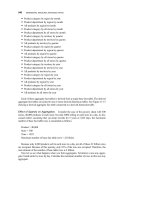
Deferred Data Extraction. In the cases discussed above, data capture takes place while
the transactions occur in the source operational systems. The data capture is immediate or
real-time. In contrast, the techniques under deferred data extraction do not capture the
changes in real time. The capture happens later. Please see Figure 12-6 showing the de-
ferred data extraction options.
268
DATA EXTRACTION, TRANSFORMATION, AND LOADING
Now let us discuss the two options for deferred data extraction.
Capture Based on Date and Time Stamp. Every time a source record is created or up-
dated it may be marked with a stamp showing the date and time. The time stamp provides
the basis for selecting records for data extraction. Here the data capture occurs at a later

time, not while each source record is created or updated. If you run your data extraction
program at midnight every day, each day you will extract only those with the date and
time stamp later than midnight of the previous day. This technique works well if the num-
ber of revised records is small.
Of course, this technique presupposes that all the relevant source records contain date
and time stamps. Provided this is true, data capture based on date and time stamp can
work for any type of source file. This technique captures the latest state of the source data.
Any intermediary states between two data extraction runs are lost.
Deletion of source records presents a special problem. If a source record gets deleted in
between two extract runs, the information about the delete is not detected. You can get
around this by marking the source record for delete first, do the extraction run, and then
go ahead and physically delete the record. This means you have to add more logic to the
source applications.
Capture by Comparing Files. If none of the above techniques are feasible for specific
source files in your environment, then consider this technique as the last resort. This tech-
nique is also called the snapshot differential technique because it compares two snapshots
of the source data. Let us see how this technique works.
Suppose you want to apply this technique to capture the changes to your product data.
DATA EXTRACTION
269
SOURCE DATABASES
SOURCE
OPERATIONAL
SYSTEMS
Today’s
Extract
Extract
Files based
on time
-

stamp
Source
Data
DBMS
OPTION 1:
Capture based
on date and time
stamp
EXTRACT
PROGRAMS
Yesterday’s
Extract
FILE
COMPARISON
PROGRAMS
Extract
Files based
on file
comparison
OPTION 2:
Capture by
comparing files
Figure 12-6 Deferred data extraction: options.
DATA STAGING AREA
While performing today’s data extraction for changes to product data, you do a full file
comparison between today’s copy of the product data and yesterday’s copy. You also com-
pare the record keys to find the inserts and deletes. Then you capture any changes be-
tween the two copies.
This technique necessitates the keeping of prior copies of all the relevant source data.
Though simple and straightforward, comparison of full rows in a large file can be very in-

efficient. However, this may be the only feasible option for some legacy data sources that
do not have transaction logs or time stamps on source records.
Evaluation of the Techniques
To summarize, the following options are available for data extraction:
ț Capture of static data
ț Capture through transaction logs
ț Capture through database triggers
ț Capture in source applications
ț Capture based on date and time stamp
ț Capture by comparing files
You are faced with some big questions. Which ones are applicable in your environ-
ment? Which techniques must you use? You will be using the static data capture technique
at least in one situation when you populate the data warehouse initially at the time of de-
ployment. After that, you will usually find that you need a combination of a few of these
techniques for your environment. If you have old legacy systems, you may even have the
need for the file comparison method.
Figure 12-7 highlights the advantages and disadvantages of the different techniques.
Please study it carefully and use it to determine the techniques you would need to use in
your environment.
Let us make a few general comments. Which of the techniques are easy and inexpen-
sive to implement? Consider the techniques of using transaction logs and database trig-
gers. Both of these techniques are already available through the database products. Both
are comparatively cheap and easy to implement. The technique based on transaction logs
is perhaps the most inexpensive. There is no additional overhead on the source operational
systems. In the case of database triggers, there is a need to create and maintain trigger
programs. Even here, the maintenance effort and the additional overhead on the source
operational systems are not that much compared to other techniques.
Data capture in source systems could be the most expensive in terms of development
and maintenance. This technique needs substantial revisions to existing source systems.
For many legacy source applications, finding the source code and modifying it may not

be feasible at all. However, if the source data does not reside on database files and date
and time stamps are not present in source records, this is one of the few available op-
tions.
What is the impact on the performance of the source operational systems? Certainly,
the deferred data extraction methods have the least impact on the operational systems.
Data extraction based on time stamps and data extraction based on file comparisons are
performed outside the normal operation of the source systems. Therefore, these two are
270
DATA EXTRACTION, TRANSFORMATION, AND LOADING