ENERGY MANAGEMENT HANDBOOKS phần 10 doc
Bạn đang xem bản rút gọn của tài liệu. Xem và tải ngay bản đầy đủ của tài liệu tại đây (3.73 MB, 87 trang )
THERMAL SCIENCES REVIEW 823
A convenient way of describing the condition of
atmospheric air is to defi ne four temperatures: dry-bulb,
wet-bulb, dew-point, and adiabatic saturation tempera-
tures. The dry-bulb temperature is simply that tempera-
ture which would be measured by any of several types
of ordinary thermometers placed in atmospheric air.
The dew-point temperature (point 2 on Figure
I.3) is the saturation temperature of the water vapor at
its existing partial pressure. In physical terms it is the
mixture temperature where water vapor would begin to
condense if cooled at constant pressure. If the relative
humidity is 100% the dew-point and dry-bulb tempera-
tures are identical.
In atmospheric air with relative humidity less
than 100%, the water vapor exists at a pressure lower
than saturation pressure. Therefore, if the air is placed
in contact with liquid water, some of the water would
be evaporated into the mixture and the vapor pressure
would be increased. If this evaporation were done in an
insulated container, the air temperature would decrease,
since part of the energy to vaporize the water must come
from the sensible energy in the air. If the air is brought
to the saturated condition, it is at the adiabatic satura-
tion temperature.
A psychrometric chart is a plot of the properties of
atmospheric air at a fi xed total pressure, usually 14.7 psia.
The chart can be used to quickly determine the properties
of atmospheric air in terms of two independent proper-
ties, for example, dry-bulb temperature and relative hu-
midity. Also, certain types of processes can be described
on the chart. Appendix II contains a psychrometric chart
for 14.7-psia atmospheric air. Psychrometric charts can
also be constructed for pressures other than 14.7 psia.
I.3 HEAT TRANSFER
Heat transfer is the branch of engineering science
that deals with the prediction of energy transport caused
by temperature differences. Generally, the fi eld is broken
down into three basic categories: conduction, convec-
tion, and radiation heat transfer.
Conduction is characterized by energy transfer by
internal microscopic motion such as lattice vibration and
electron movement. Conduction will occur in any region
where mass is contained and across which a tempera-
ture difference exists.
Convection is characterized by motion of a fl uid
region. In general, the effect of the convective motion is
to augment the conductive effect caused by the existing
temperature difference.
Radiation is an electromagnetic wave transport
phenomenon and requires no medium for transport. In
fact, radiative transport is generally more effective in a
vacuum, since there is attenuation in a medium.
I.3.1 Conduction Heat Transfer
The basic tenet of conduction is called Fourier’s
law,
Q =–kA
dT
dx
The heat fl ux is dependent upon the area across which
energy fl ows and the temperature gradient at that plane.
The coeffi cient of proportionality is a material property,
called thermal conductivity k. This relationship always
applies, both for steady and transient cases. If the gradi-
ent can be found at any point and time, the heat fl ux
density,
Q/A
, can be calculated.
Conduction Equation. The control volume ap-
proach from thermodynamics can be applied to give an
energy balance which we call the conduction equation.
For brevity we omit the details of this development; see
Refs. 2 and 3 for these derivations. The result is
G + K∇
2
T =–ρC
∂T
∂τ
(I.4)
This equation gives the temperature distribution in
space and time, G is a heat-generation term, caused
by chemical, electrical, or nuclear effects in the control
volume. Equation I.4 can be written
∇
2
T +
G
K
=
ρC
k
∂T
∂τ
The ratio k/ρC is also a material property called thermal
diffusivity u. Appendix II gives thermophysical proper-
ties of many common engineering materials.
For steady, one-dimensional conduction with no
heat generation,
Fig. I.3 Behavior of water in air: φ = P
1
/P
3
; T
2
= dew
point.
s
T
P
3
P
1
3
1
2
824 ENERGY MANAGEMENT HANDBOOK
D
2
T
dx
2
=0
This will give T = ax + b, a simple linear relationship
between temperature and distance. Then the application
of Fourier’s law gives
Q = kA
T
x
a simple expression for heat transfer across the ∆x dis-
tance. If we apply this concept to insulation for example,
we get the concept of the R value. R is just the resistance
to conduction heat transfer per inch of insulation thick-
ness (i.e., R = 1/k).
Multilayered, One-Dimensional Systems. In
practical applications, there are many systems that can
be treated as one-dimensional, but they are composed
of layers of materials with different conductivities. For
example, building walls and pipes with outer insulation
fi t this category. This leads to the concept of overall
heat-transfer coeffi cient, U. This concept is based on the
defi nition of a convective heat-transfer coeffi cient,
Q = hA T
This is a simplifi ed way of handling convection at a
boundary between solid and fl uid regions. The heat-
transfer coeffi cient h represents the infl uence of fl ow
conditions, geometry, and thermophysical properties on
the heat transfer at a solid-fl uid boundary. Further dis-
cussion of the concept of the h factor will be presented
later.
Figure I.4 represents a typical one-dimensional,
multilayered application. We define an overall heat-
transfer coeffi cient U as
Q = UA (T
i
– T
o
)
We fi nd that the expression for U must be
U =
1
1
h
1
+
x
1
k
1
+
x
2
k
2
+
x
3
k
3
+
1
h
0
This expression results from the application of the
conduction equation across the wall components and
the convection equation at the wall boundaries. Then,
by noting that in steady state each expression for heat
must be equal, we can write the expression for U, which
contains both convection and conduction effects. The U
factor is extremely useful to engineers and architects in
a wide variety of applications.
The U factor for a multilayered tube with convec-
tion at the inside and outside surfaces can be developed
in the same manner as for the plane wall. The result is
U =
1
1
h
0
+
r
0
ln r
j
+1/r
j
k
j
ΣΣ
j
+
1r
0
h
i
r
i
where r
i
and r
o
are inside and outside radii.
Caution: The value of U depends upon which radius you
choose (i.e., the inner or outer surface).
If the inner surface were chosen, we would get
U =
1
1r
i
h
0
r
0
+
r
i
ln r
j
+1/r
j
k
j
ΣΣ
j
+
1
h
i
However, there is no difference in heat-transfer rate;
that is,
Q
o
= U
i
A
i
T
overall
= U
o
A
o
T
overall
so it is apparent that
U
i
A
i
= U
o
A
o
for cylindrical systems.
Finned Surfaces. Many heat-exchange surfaces
experience inadequate heat transfer because of low
heat-transfer coeffi cients between the surface and the
adjacent fl uid. A remedy for this is to add material to
the surface. The added material in some cases resembles
a fi sh “fi n,” thereby giving rise to the expression “a
fi nned surface.” The performance of fi ns and arrays of
fi ns is an important item in the analysis of many heat-ex-
change devices. Figure I.5 shows some possible shapes
for fi ns.
Fig. I.4 Multilayered wall with convection at the inner
and outer surfaces.
THERMAL SCIENCES REVIEW 825
The analysis of fi ns is based on a simple energy
balance between one-dimensional conduction down
the length of the fi n and the heat convected from the
exposed surface to the surrounding fluid. The basic
equation that applies to most fi ns is
d
2
θ 1dA dθ h 1 dS
—— + ———— – ——— θ = 0 (I.5)
dx
2
A dx dx k A dx
when θ is (T – T
∞
), the temperature difference between
fi n and fl uid at any point; A is the cross-sectional area
of the fi n; S is the exposed area; and x is the distance
along the fi n. Chapman
2
gives an excellent discussion
of the development of this equation.
The application of equation I.5 to the myriad of
possible fi n shapes could consume a volume in itself.
Several shapes are relatively easy to analyze; for ex-
ample, fi ns of uniform cross section and annular fi ns can
be treated so that the temperature distribution in the fi n
and the heat rate from the fi n can be written. Of more
utility, especially for fi n arrays, are the concepts of fi n
effi ciency and fi n surface effectiveness (see Holman
3
).
Fin effi ciency η
ƒ
is defi ned as the ratio of actual
heat loss from the fi n to the ideal heat loss that would
occur if the fi n were isothermal at the base temperature.
Using this concept, we could write
Q
fin
= A
fin
h
T
b
– T
Ü
η
f
η
ƒ
is the factor that is required for each case. Figure I.6
shows the fi n effi ciency for several cases.
Surface effectiveness K is defi ned as the actual heat
transfer from a fi nned surface to that which would occur
if the surface were isothermal at the base temperature.
Taking advantage of fi n effi ciency, we can write
(A – A
f
)h θ
0
+ η
f
A
f
θ
0
K = —————————— (I.6)
A
h
θ
0
Equation I.6 reduces to
A
f
K = 1 —— (1 – η
f
)
A
which is a function only of geometry and single fi n ef-
fi ciency. To get the heat rate from a fi n array, we write
Q
array
= Kh (T
b
– T
∞
) A
where A is the total area exposed.
Transient Conduction. Heating and cooling prob-
lems involve the solution of the time-dependent conduc-
tion equation. Most problems of industrial signifi cance
occur when a body at a known initial temperature is
suddenly exposed to a fl uid at a different temperature.
The temperature behavior for such unsteady problems
can be characterized by two dimensionless quantities,
the Biot number, Bi = hL/k, and the Fourier modulus,
Fo = ατ/L
2
. The Biot number is a measure of the ef-
fectiveness of conduction within the body. The Fourier
modulus is simply a dimensionless time.
If Bi is a small, say Bi ≤ 0.1, the body undergoing
the temperature change can be assumed to be at a uni-
form temperature at any time. For this case,
T – T
f
T
i
– T
f
= exp –
hA
ρCV
τ
where T
ƒ
and T
i
are the fl uid temperature and initial
body temperature, respectively. The term (ρCV/hA) takes
on the characteristics of a time constant.
If Bi ≥ 0.1, the conduction equation must be solved
in terms of position and time. Heisler
4
solved the equa-
tion for infi nite slabs, infi nite cylinders, and spheres. For
convenience he plotted the results so that the tempera-
ture at any point within the body and the amount of
heat transferred can be quickly found in terms of Bi and
Fo. Figures I.7 to I.10 show the Heisler charts for slabs
and cylinders. These can be used if h and the properties
of the material are constant.
Fig. I.5 Fins of various shapes. (a) Rectangular, (b) Trap-
ezoidal, (c) Arbitrary profi le, (d ) Circumferential.
826 ENERGY MANAGEMENT HANDBOOK
I.3.2 Convection Heat Transfer
Convective heat transfer is considerably more com-
plicated than conduction because motion of the medium
is involved. In contrast to conduction, where many geo-
metrical confi gurations can be solved analytically, there
are only limited cases where theory alone will give
convective heat-transfer relationships. Consequently,
convection is largely what we call a semi-empirical sci-
ence. That is, actual equations for heat transfer are based
strongly on the results of experimentation.
Convection Modes. Convection can be split into
several subcategories. For example, forced convection
refers to the case where the velocity of the fl uid is com-
pletely independent of the temperature of the fl uid. On
the other hand, natural (or free) convection occurs when
the temperature fi eld actually causes the fl uid motion
through buoyancy effects.
We can further separate convection by
geometry into external and internal fl ows. Inter-
nal refers to channel, duct, and pipe fl ow and
external refers to unbounded fl uid fl ow cases.
There are other specialized forms of convection,
for example the change-of-phase phenomena:
boiling, condensation, melting, freezing, and so
on. Change-of-phase heat transfer is diffi cult to
predict analytically. Tongs
5
gives many of the
correlations for boiling and two-phase fl ow.
Dimensional Heat-Transfer Parameters.
Because experimentation has been required to
develop appropriate correlations for convective
heat transfer, the use of generalized dimension-
less quantities in these correlations is preferred.
In this way, the applicability of experimental
data covers a wider range of conditions and fl u-
ids. Some of these parameters, which we gener-
ally call “numbers,” are given below:
hL
Nusselt number: Nu = ——
k
where k is the fl uid conductivity and L is mea-
sured along the appropriate boundary between
liquid and solid; the Nu is a nondimensional
heat-transfer coeffi cient.
Lu
Reynolds number: Re = ——
υ
defi ned in Section I.4: it controls the character
of the fl ow
Cμ
Prandtl number: Pr = ——
k
ratio of momentum transport to heat-transport charac-
teristics for a fl uid: it is important in all convective cases,
and is a material property
g β(T – T
∞
)L
3
Grashof number: Gr = ——————
υ
2
serves in natural convection the same role as Re in
forced convection: that is, it controls the character of
the fl ow
h
Stanton number: St = ———
ρ uC
p
Fig. I.6 (a) Effi ciencies of rectangular and triangular fi ns, (b) Ef-
fi ciencies of circumferential fi ns of rectangular profi le.
THERMAL SCIENCES REVIEW 827
also a nondimensional heat-transfer coeffi cient: it is very
useful in pipe fl ow heat transfer.
In general, we attempt to correlate data by using
relationships between dimensionless numbers: for ex-
ample, in many convection cases, we could write Nu =
Nu(Re, Pr) as a functional relationship. Then it is pos-
sible either from analysis, experimentation, or both, to
write an equation that can be used for design calcula-
tions. These are generally called working formulas.
Forced Convection Past Plane Surfaces. The aver-
age heat-transfer coeffi cient for a plate of length L may
be calculated from
Nu
L
= 0.664 (Re
L
)
1/2
(Pr)
1/3
if the fl ow is laminar (i.e., if Re
L
≤ 4,000). For this case
the fl uid properties should be evaluated at the mean
fi lm temperature T
m
, which is simply the arithmetic
Fig. I.7 Midplane temperature for an infi nite plate of thickness 2L. (From Ref. 4.)
Fig. I.8 Axis temperature for an infi nite cylinder of radius r
o
. (From Ref. 4.)
828 ENERGY MANAGEMENT HANDBOOK
average of the fl uid and the surface temperature.
For turbulent fl ow, there are several acceptable cor-
relations. Perhaps the most useful includes both laminar
leading edge effects and turbulent effects. It is
Nu = 0.0036 (Pr)
1/3
[(Re
L
)
0.8
– 18.700]
where the transition Re is 4,000.
Forced Convection Inside Cylindrical Pipes or
Tubes. This particular type of convective heat trans-
fer is of special engineering signifi cance. Fluid fl ows
through pipes, tubes, and ducts are very prevalent, both
in laminar and turbulent fl ow situations. For example,
most heat exchangers involve the cooling or heating of
fl uids in tubes. Single pipes and/or tubes are also used
to transport hot or cold liquids in industrial processes.
Most of the formulas listed here are for the 0.5 ≤ Pr ≤
100 range.
Laminar Flow. For the case where Re
D
< 2300,
Nusselt showed that Nu
D
= 3.66 for long tubes at a
constant tube-wall temperature. For forced convection
cases (laminar and turbulent) the fl uid properties are
evaluated at the bulk temperature T
b
. This temperature,
also called the mixing-cup temperature, is defi ned by
T
b
=
uTr dr
0
R
ur dr
0
R
if the properties of the fl ow are constant.
Sieder and Tate developed the following more
convenient empirical formula for short tubes:
Nu
D
=1.86 Re
D
1/3
Pr
1/3
D
L
1/3
Ç
Ç
s
0.14
The fl uid properties are to be evaluated at T
b
except for
the quantity μ
s
, which is the dynamic viscosity evalu-
ated at the temperature of the wall.
Turbulent Flow. McAdams suggests the empirical
relation
Nu
D
= 0.023 (Pr
D
)
0.8
(Pr)
n
(I.7)
where n = 0.4 for heating and n = 0.3 for cooling. Equa-
tion I.7 applies as long as the difference between the
pipe surface temperature and the bulk fl uid temperature
is not greater than 10°F for liquids or 100°F for gases.
For temperature differences greater then the limits
specifi ed for equation I.7 or for fl uids more viscous than
water, the following expression from Sieder and Tate
will give better results:
NU
D
= 0.027 Pr
D
0.8
Pr
1/3
Ç
Ç
s
0.14
Note that the McAdams equation requires only a knowl-
edge of the bulk temperature, whereas the Sieder-Tate
expression also requires the wall temperature. Many
people prefer equation I.7 for that reason.
Fig. I.9 Temperature as a function of center temperature
in an infi nite plate of thickness 2L. (From Ref. 4.)
Fig. I.10 Temperature as a function of axis temperature in
an infi nite cylinder of radius r
o
. (From Ref. 4.)
THERMAL SCIENCES REVIEW 829
Nusselt found that short tubes could be repre-
sented by the expression
Nu
D
= 0.036 Pe
D
0.8
Pr
1/3
Ç
Ç
s
0.14
D
L
1/18
For noncircular ducts, the concept of equivalent diam-
eter can be employed, so that all the correlations for
circular systems can be used.
Forced Convection in Flow Normal to Single
Tubes and Banks. This circumstance is encountered
frequently, for example air fl ow over a tube or pipe
carrying hot or cold fl uid. Correlations of this phenom-
enon are called semi-empirical and take the form Nu
D
= C(Re
D
)
m
. Hilpert, for example, recommends the values
given in Table I.8. These values have been in use for
many years and are considered accurate.
Flows across arrays of tubes (tube banks) may be
even more prevalent than single tubes. Care must be
exercised in selecting the appropriate expression for the
tube bank. For example, a staggered array and an in-line
array could have considerably different heat-transfer
characteristics. Kays and London
6
have documented
many of these cases for heat-exchanger applications. For
a general estimate of order-of-magnitude heat-transfer
coeffi cients, Colburn’s equation
Nu
D
= 0.33 (Re
D
)
0.6
(Pr)
1/3
is acceptable.
Free Convection Around Plates and Cylinders.
In free convection phenomena, the basic relationships
take on the functional form Nu = ƒ(Gr, Pr). The Grashof
number replaces the Reynolds number as the driving
function for fl ow.
In all free convection correlations it is customary to
evaluate the fl uid properties at the mean fi lm tempera-
ture T
m
, except for the coeffi cient of volume expansion
β, which is normally evaluated at the temperature of the
undisturbed fl uid far removed from the surface—name-
ly, T
ƒ
. Unless otherwise noted, this convention should be
used in the application of all relations quoted here.
Table I.9 gives the recommended constants and ex-
ponents for correlations of natural convection for vertical
plates and horizontal cylinders of the form Nu = C
• Ra
m
.
The product Gr • Pr is called the Rayleigh number (Ra)
and is clearly a dimensionless quantity associated with
any specifi c free convective situation.
I.3.3 Radiation Heat Transfer
Radiation heat transfer is the most mathematically
complicated type of heat transfer. This is caused pri-
marily by the electromagnetic wave nature of thermal
radiation. However, in certain applications, primarily
high-temperature, radiation is the dominant mode of
heat transfer. So it is imperative that a basic understand-
ing of radiative heat transport be available. Heat transfer
in boiler and fi red-heater enclosures is highly dependent
upon the radiative characteristics of the surface and the
hot combustion gases. It is known that for a body radiat-
ing to its surroundings, the heat rate is
Q = εσAT
4
– T
s
4
where ε is the emissivity of the surface, σ is the Stefan-
Boltzmann constant, σ = 0.1713 × 10
– 8
Btu/hr ft
2
• R
4
.
Temperature must be in absolute units, R or K. If ε = 1
for a surface, it is called a “blackbody,” a perfect emit-
ter of thermal energy. Radiative properties of various
surfaces are given in Appendix II. In many cases, the
heat exchange between bodies when all the radiation
emitted by one does not strike the other is of interest.
In this case we employ a shape factor F
ij
to modify the
basic transport equation. For two blackbodies we would
write
Q
12
= F
12
σAT
1
4
– T
2
4
Table I.8 Values of C and m for Hilpert’s Equation
Range of N
Re
D
C m
1-4 0.891 0.330
4-40 0.821 0.385
40-4000 0.615 0.466
4000-40,000 0.175 0.618
40,000-250,000 0.0239 0.805
Table I.9 Constants and Exponents
for Natural Convection Correlations
Vertical Plate
a
Horizontal Cylinders
b
Ra c m c m
10
4
< Ra < 10
9
0.59 1/4 0.525 1/4
10
9
< Ra < 10
12
0.129 1/3 0.129 1/3
a
Nu and Ra based on vertical height L.
b
Nu and Ra based on diameter D.
830 ENERGY MANAGEMENT HANDBOOK
for the heat transport from body 1 to body 2. Figures
I.11 to I.14 show the shape factors for some commonly
encountered cases. Note that the shape factor is a func-
tion of geometry only.
Gaseous radiation that occurs in luminous com-
bustion zones is diffi cult to treat theoretically. It is too
complex to be treated here and the interested reader is
referred to Siegel and Howell
7
for a detailed discussion.
I.4 FLUID MECHANICS
In industrial processes we deal with materials that
can be made to fl ow in a conduit of some sort. The laws
that govern the fl ow of materials form the science that
is called fl uid mechanics. The behavior of the fl owing
fl uid controls pressure drop (pumping power), mixing
effi ciency, and in some cases the effi ciency of heat trans-
fer. So it is an integral portion of an energy conservation
program.
I.4.1 Fluid Dynamics
When a fl uid is caused to fl ow, certain governing
laws must be used. For example, mass fl ows in and out
of control volumes must always be balanced. In other
words, conservation of mass must be satisfi ed.
In its most basic form the continuity equation
(conservation of mass) is
c.s. c.v.
In words, this is simply a balance between mass enter-
ing and leaving a control volume and the rate of mass
storage. The ρ(
υ
•
n
) terms are integrated over the control
surface, whereas the ρ dV term is dependent upon an
integration over the control volume.
For a steady fl ow in a constant-area duct, the con-
tinuity equation simplifi es to
m = ρ
f
Α
c
u = constant
That is, the mass fl ow rate
m
is constant and is equal to
the product of the fl uid density ρ
ƒ
, the duct cross section
A
c
, and the average fl uid velocity
u
.
If the fl uid is compressible and the fl ow is steady,
one gets
m
ρ
f
= constant = u
Α
c
u
Α
c
2
where 1 and 2 refer to different points in a variable
area duct.
I.4.2 First Law—Fluid Dynamics
The fi rst law of thermodynamics can be directly
applied to fl uid dynamical systems, such as duct fl ows.
If there is no heat transfer or chemical reaction and if the
internal energy of the fl uid stream remains unchanged,
the fi rst law is
V
i
2
_ V
e
2
2g
c
+
z
i
– z
e
g
c
g +
p
i
– p
e
ρ
+ w
p
– w
f
=0
(I.8)
Fig. I.11 Radiation shape factor for perpendicular rectangles with a common edge.
ÌÌ
ÌÌÌ
ρυ [
•
n dA +
∂
∂
t
ρ dV =0
THERMAL SCIENCES REVIEW 831
In the English system, horsepower is
hp = m
lb
m
sec
w
p
=
ft
•
lb
f
lb
m
×
1 hp – sec
500 ft – lb
=
mw
p
550
Referring back to equation I.8, the most diffi cult term to
determine is usually the frictional work term w
ƒ
. This is
a term that depends upon the fl uid viscosity, the fl ow
conditions, and the duct geometry. For simplicity, w
ƒ
is
generally represented as
p
f
w
f
= ——
ρ
when ∆p
ƒ
is the frictional pressure drop in the duct.
Further, we say that
p
f
ρ
=
2 fu
2
L
g
c
D
in a duct of length L and diameter D. The friction factor
ƒ is a convenient way to represent the differing infl uence
of laminar and turbulent fl ows on the friction pressure
drop.
Fig. I.13 Radiation shape factor for concentric cylinders
of fi nite length.
Fig. I.14 Radiation shape factor for parallel, directly
opposed rectangles.
where the subscripts i and e refer to inlet and exit condi-
tions and w
p
and w
ƒ
are pump work and work required
to overcome friction in the duct. Figure I.15 shows sche-
matically a system illustrating this equation.
Any term in equation I.8 can be converted to a rate
expression by simply multiplying by , the mass fl ow
rate. Take, for example, the pump horsepower,
W
energy
time
= mw
p
mass
time
energy
mass
Fig. I.12 Radiation shape factor for parallel, concentric
disks.
Fig. I.15 The fi rst law applied to adiabatic fl ow system.
832 ENERGY MANAGEMENT HANDBOOK
The character of the fl ow is deter-
mined through the Reynolds number,
Re = ρuD/μ, where μ is the viscosity of
the fl uid. This nondimensional group-
ing represents the ratio of dynamic to
viscous forces acting on the fl uid.
Experiments have shown that if Re
≤ 2300, the fl ow is laminar. For larger Re
the fl ow is turbulent. Figure I.16 shows
how the friction factor depends upon
the Re of the fl ow. Note that for laminar
fl ow the ƒ vs. Re curve is single-valued
and is simply equal to 16/Re. In the
turbulent regime, the wall roughness e
can affect the friction factor because of
its effect on the velocity profi le near the
duct surface.
If a duct is not circular, the equiva-
lent diameter D
e
can be used so that all
the relationships developed for circular
systems can still be used. D
e
is defi ned as
4A
c
D
e
= ——
P
P is the “wetted” perimeter, that part of the fl ow cross
section that touches the duct surfaces. For a circular
system D
e
= 4(πD
2
/4πD) = D, as it should. For an an-
nular duct, we get
D
e
=
ÉD
o
2
⁄ 4–ÉD
i
2
⁄ 44
ÉD
o
+ ÉD
i
=
É D
o
+ D
i
D
o
+ D
i
ÉD
o
+ ÉD
i
= D
o
+ D
i
Pressure Drop in Ducts. In practical applications,
the essential need is to predict pressure drops in piping
and duct networks. The friction factor approach is ad-
equate for straight runs of constant area ducts. But valves
nozzles, elbows, and many other types of fi ttings are nec-
essarily included in a network. This can be accounted for
by defi ning an equivalent length L
e
for the fi tting. Table
I.10 shows L
e/
D values for many different fi ttings.
Pressure Drop across Tube Banks. Another com-
monly encountered application of fl uid dynamics is the
pressure drop caused by transverse fl ow across arrays
of heat-transfer tubes. One technique to calculate this
effect is to fi nd the velocity head loss through the tube
bank:
N
v
= ƒNF
d
where ƒ is the friction factor for the tubes (a function
of the Re), N the number of tube rows crossed by the
fl ow, and F
d
is the “depth factor.” Figures I.17 and I.18
show the ƒ factor and F
d
relationship that can be used in
pressure-drop calculations. If the fl uid is air, the pressure
drop can be calculated by the equation
p = N
30
B
T
1.73 × 10
5
G
10
3
2
where B is the atmospheric pressure (in. Hg), T is tem-
perature (°R), and G is the mass velocity (lbm/ft
2
hr).
Bernoulli’s Equation. There are some cases where the
equation
p u
2
— + — + gz = constant
ρ 2
which is called Bernoulli’s equation, is useful. Strictly
speaking, this equation applies for inviscid, incompress-
ible, steady fl ow along a streamline. However, even in
pipe fl ow where the fl ow is viscous, the equation can
be applied because of the confi ned nature of the fl ow.
That is, the fl ow is forced to behave in a streamlined
manner. Note that the first law equation (I.8) yields
Bernoulli’s equation if the friction drop exactly equals
the pump work.
I.4.3 Fluid-Handling Equipment
For industrial processes, another prime applica-
tion of fl uid dynamics lies in fl uid-handling equipment.
Fig. I.16 Friction factors for straight pipes.
THERMAL SCIENCES REVIEW 833
Pumps, compressors, fans, and blowers are extensively
used to move gases and liquids through the process
network and over heat-exchanger surfaces. The general
constraint in equipment selection is a matching of fl uid
handler capacity to pressure drop in the circuit con-
nected to the fl uid handler.
Pumps are used to transport liquids, whereas
compressors, fans, and blowers apply to gases. There
are features of performance common to all of them. For
purposes of illustration, a centrifugal pump will be used
to discuss performance characteristics.
Centrifugal Machines. Centrifugal machines op-
erate on the principle of centrifugal acceleration of a
fl uid element in a rotating impeller/housing system to
achieve a pressure gain and circulation.
The characteristics that are important are fl ow rate
(capacity), head, effi ciency, and durability. Q
ƒ
(capac-
ity), h
p
(head), and η
p
(effi ciency) are related quantities,
dependent basically on the fl uid behavior in the pump
and the fl ow circuit. Durability is related to the wear,
corrosion, and other factors that bear on a pump’s reli-
ability and lifetime.
Figure I.19 shows the relation between fl ow rate
and related characteristics for a centrifugal pump at con-
stant speed. Graphs of this type are called performance
curves; fhp and bhp are fl uid and brake horsepower, re-
spectively. The primary design constraint is a matching
Table I.10 L
e
/D for Screwed Fittings, Turbulent
Flow Only
a
—————————————————————————
Fitting L
e
/
D
—————————————————————————
45° elbow 15
90° elbow, standard radius 31
90° elbow, medium radius 26
90° elbow, long sweep 20
90° square elbow 65
180° close return bend 75
Swing check valve, open 77
Tee (as el, entering run) 65
Tee (as el, entering branch) 90
Couplings, unions Negligible
Gate valve, open 7
Gate valve, 1/4 closed 40
Gate valve, 1/2 closed 190
Gate valve, 3/4 closed 840
Globe valve, open 340
Angle valve, open 170
—————————————————————————
a
Calculated from Crane Co. Tech. Paper 409, May 1942.
Fig. I.17 Depth factor for number of tube rows crossed
in convection banks.
Fig. I.18 Friction factor ƒ as affected by Reynolds number
for various in-line tube patterns, crossfl ow gas or air, d
o
,
tube diameter; l
⊥
, gap distance perpendicular to the fl ow;
l
||
, gap distance parallel to the fl ow.
834 ENERGY MANAGEMENT HANDBOOK
Q
f
ρgh
p
fhp = ————
550g
c
Q
f
ρgh
p
550g
c
fhp
η
p
p = —————— = ——
bhp bhp
system effi ciency η
s
= η
p
× η
m
(motor effi ciency)
It is important to select the motor and pump so that
at nominal operating conditions, the pump and motor
operate at near their maximum effi ciency.
For systems where two or more pumps are pres-
ent, the following rules are helpful. To analyze pumps
in parallel, add capacities at the same head. For pumps
in series, simply add heads at the same capacity.
There is one notable difference between blowers
and pump performance. This is shown in Figure I.20.
Note that the bhp continues to increase as permissible
head goes to zero, in contrast to the pump curve when
bhp approaches zero. This is because the kinetic energy
imparted to the fl uid at high fl ow rates is quite signifi -
cant for blowers.
Manufactures of fl uid-handling equipment provide
excellent performance data for all types of equipment.
Anyone considering replacement or a new installation
should take full advantage of these data.
Fluid-handling equipment that operates on a prin-
ciple other than centrifugal does not follow the centrifu-
gal scaling laws. Evans
8
gives a thorough treatment of
most types of equipment that would be encountered in
industrial application.
of fl ow rate to head. Note that as the fl ow-rate require-
ment is increased, the allowable head must be reduced
if other pump parameters are unchanged.
Analysis and experience has shown that there are
scaling laws for centrifugal pump performance that give
the trends for a change in certain performance param-
eters. Basically, they are:
Effi ciency:
η
p
=ƒ
1
Q
f
D
3
n
Dimensionless head:
h
p
g
D
2
n
2
= f
2
Q
f
D
3
n
Dimensionless brake horsepower:
bhp
•
g
γD
2
n
3
= f
3
Q
f
D
3
n
where D is the impeller diameter, n is the rotary impel-
ler speed, g is gravity, and γ is the specifi c weight of
fl uid.
The basic relationships yield specifi c proportionali-
ties such as Q
ƒ
∝ n (rpm), h
p
∝ n
2
, fhp ∝ n
3
,
Q
f
∝
1
D
2
,
h
p
∝
1
D
4
, and
fh
p
∝
1
D
4
.
For pumps, density variations are generally negli-
gible since liquids are incompressible. But for gas-han-
dling equipment, density changes are very important.
The scaling laws will give the following rules for chang-
ing density:
h
p
∝ ρ
fh
p
∝ ρ (Q
f
, n constant)
n
fhp
Q
f
∝ρ !
–1/2
(h
p
constant
n
Q
f
h
p
∝
1
ρ
(
m
constant)
1
fhp ∝ ——
ρ
2
For centrifugal pumps, the following equations hold:
Fig. I.19 Performance curve for a centrifugal pump.
THERMAL SCIENCES REVIEW 835
References
1. G.J. Van Wylen and R.E. Sonntag, Fundamentals of Classical
Thermodynamics, 2nd ed., Wiley, New York, 1973.
2. A.S. Chapman, Heat Transfer, 3rd ed., Macmillan, New York,
1974.
3. J.P. Holman, Heat Transfer, 4th ed., McGraw-Hill, New York,
1976.
4. M.P. Heisler, Trans. ASME, Vol. 69 (1947), p. 227.
5. L.S. Tong, Boiling Heat Transfer and Two-Phase Flow, Wiley,
New York, 1965.
6. W.M. Kays and A.L. London, Compact Heat Exchangers, 2nd
ed., McGraw-Hill, New York, 1963.
7. R. Siegel and J.R. Howell, Thermal Radiation Heat Transfer,
McGraw-Hill, New York, 1972.
8. FRANK L. Evans, JR., Equipment Design Handbook for Re-
fi neries and Chemical Plants, Vols. 1 and 2, Gulf Publishing,
Houston, Tex., 1974.
SYMBOLS
Thermodynamics
AF air/fuel ratio
C
p
constant-pressure specifi c heat
C
v
constant-volume specifi c heat
C
p
0
zero-pressure constant-pressure specifi c heat
C
v0
zero-pressure constant-volume specufi c heat
e, E specifi c energy and total energy
g acceleration due to gravity
g, G specifi c Gibbs function and total Gibbs func-
tion
g
e
a constant that relates force, mass, length, and
time
h, H specifi c enthalpy and total enthalpy
k specifi c heat ratio: C
p
/C
v
K.E. kinetic energy
lb
f
pound force
lb
m
pound mass
lb mol pound mole
m mass
m
mass rate of fl ow
M molecular weight
n number of moles
n polytropic exponent
P pressure
P
i
partial pressure of component i in a mixture
P.E. potential energy
P
r
relative pressure as used in gas tables
q, Q heat transfer per unit mass and total heat
transfer
Q
rate of heat transfer
Q
H, QL heat transfer from high- and low-temperature
bodies
R gas constant
R universal gas constant
s, S specifi c entropy and total entropy
t time
T temperature
u, U specific internal energy and total internal
energy
v, V specifi c volume and total volume
V velocity
V
r
relative velocity
w, W work per unit mass and total work
W rate of work, or power
w
rev
reversible work between two states assuming
heat transfer with surroundings
x mass fraction
Z elevation
Z compressibility factor
Greek Letters
β coeffi cient of performance for a refrigerator
β' coeffi cient of performance for a heat pump
η effi ciency
ρ density
φ relative humidity
ω humidity ratio or specifi c humidity
Subscripts
c property at the critical point
c.v. control volume
e state of a substance leaving a control vol-
ume
ƒ formation
ƒ property of saturated liquid
ƒg difference in property for saturated vapor
Fig. I.20 Variation of head and bhp with fl ow rate for a
typical blower at constant speed.
836 ENERGY MANAGEMENT HANDBOOK
and saturated liquid
g property of saturated vapor
r reduced property
s isentropic process
Superscripts
- bar over symbol denotes property on a molal
basis (over V, H, S, U, A, G, the bar denotes
partial molal property)
° property at standard-state condition
* ideal gas
L liquid phase
S solid phase
V vapor phase
Heat Transfer—Fluid Flow
A surface area
A
m
profi le area for a fi n
Bi Biot number, (hL/k)
c
p
specifi c heat at constant pressure
c specifi c heat
D diameter
D
e
hydraulic diameter
F
i-j
shape factor of area i with respect to area j
ƒ friction factor
Gr Grashof number,
g βÄTL
c
3
/υ
2
g acceleration due to gravity
g
c
gravitational constant
h convective heat-transfer coeffi cient
k thermal conductivity
m mass
m
mass rate of fl ow
N number of rows
Nu Nusselt number, hL/k
Pr Prandtl number, μC
p
/k
p pressure
Q
volumetric fl ow rate
Q rate of heat fl ow
Ra Rayleigh number,
g βÄTL
c
3
/υ∝
Re Reynolds number, ρu
av
L
c
/μ
r radius
St Stanton number, h/Cp ρu
∝
T temperature
U overall heat-transfer coeffi cient
u velocity
ux free-stream velocity
V volume
V velocity
W rate of work done
Greek Symbols
α thermal diffusivity
β coeffi cient of thermal expansion
∆ difference, change
ε surface emissivity
η
f
fi n effectiveness
μ viscosity
v kinematic viscosity
ρ density
σ Stefan-Boltzmann constant
τ time
Subscripts
b bulk conditions
cr critical condition
c convection
cond conduction
conv convection
e entrance, effective
ƒ fi n, fl uid
i inlet conditions
o exterior condition
0 centerline conditions in a tube at r = 0
o outlet condition
p pipe, pump
s surface condition
∝ free-stream condition
APPENDIX II
CONVERSION FACTORS AND PROPERTY TABLES
Compiled by
L.C. WITTE
Professor of Mechanical Engineering
University of Houston
Houston, Texas
Table II.1 Conversion Factors
To Obtain: Multiply: By:
Acres Sq miles 640.0
Atmospheres Cm of Hg @ 0 deg C 0.013158
Atmospheres Ft of H
2
O @ 39.2 F. 0.029499
Atmospheres Grams/sq cm 0.00096784
Atmospheres In. Hg @ 32 F 0.033421
Atmospheres In. H
2
O @ 39.2 F 0.0024583
Atmospheres Pounds/sq ft 0.00047254
Atmospheres Pounds/sq in. 0.068046
Btu Ft-lb 0.0012854
Btu Hp-hr 2545.1
Btu Kg-cal. 3.9685
Btu kW-hr 3413
Btu Watt-hr 3.4130
Btu/(cu ft) (hr) kW/liter 96,650.6
Btu/hr Mech. hp 2545.1
Btu/hr kW 3413
Btu/hr Tons of refrigeration 12,000
Btu/hr Watts 3.4127
Btu/kW hr Kg cal/kW hr 3.9685
Btu/(hr) (ft) (deg F) Cal/(sec) (cm) (deg C) 241.90
Btu/(hr) (ft) (deg F) Joules/(sec) (cm) (deg C) 57.803
Btu/(hr) (ft) (deg F) Watts/(cm) (deg C) 57.803
Btu/(hr) (sq ft) Cal/(sec) (sq cm) 13,273.0
Btu/min Ft-lb/min 0.0012854
Btu/min Mech. hp 42.418
Btu/min kW 56.896
Btu/lb Cal/gram 1.8
Btu/lb Kg cal/kg 1.8
Btu/(lb) (deg F) Cal/(gram) (deg C) 1.0
Btu/(lb) (deg F) Joules/(gram) (deg C) 0.23889
Btu/sec Mech. hp 0.70696
Btu/sec Mech. hp (metric) 0.6971
Btu/sec Kg-cal/hr 0.0011024
Btu/sec kW 0.94827
Btu/sq ft Kg-cal/sq meter 0.36867
837
838 ENERGY MANAGEMENT HANDBOOK
Table II.1 Continued
To Obtain: Multiply: By:
Calories Ft-lb 0.32389
Calories Joules 0.23889
Calories Watt-hr 860.01
Cal/(cu cm) (sec) kW/liter 0.23888
Cal/gram Btu/lb 0.55556
Cal/(gram) (deg C) Btu/(lb) (deg F) 1.0
Cal/(sec) (cm) (deg C) Btu/(hr) (ft) (deg F) 0.0041336
Cal/(sec) (sq cm) Btu/(hr) (sq ft) 0.000075341
Cal/(sec) (sq cm) (deg C) Btu/(hr) (sq ft) (deg F) 0.0001355
Centimeters Inches 2.540
Centimeters Microns 0.0001
Centimeters Mils 0.002540
Cm of Hg @ 0 deg C Atmospheres 76.0
Cm of Hg @ 0 deg C Ft of H
2
O @ 39.2 F 2.242
Cm of Hg @ 0 deg C Grams/sq cm 0.07356
Cm of Hg @ 0 deg C In. of H
2
O @ 4 C 0.1868
Cm of Hg @ 0 deg C Lb/sq in. 5.1715
Cm of Hg @ 0 deg C Lb/sq ft 0.035913
Cm/deg C In./deg F 4.5720
Cm/sec Ft/min 0.508
Cm/sec Ft/sec 30.48
Cm/(sec) (sec) Gravity 980.665
Cm of H
2
O @39.2 F Atmospheres 1033.24
Cm of H
2
O @39.2 F Lb/sq in. 70.31
Centipoises Centistokes Density
Centistokes Centipoises l/density
Cu cm Cu ft 28,317
Cu cm Cu in. 16.387
Cu cm Gal. (USA, liq.) 3785.43
Cu cm Liters 1000 03
Cu cm Ounces (USA, liq.) 29.573730
Cu cm Quarts (USA, liq.) 946.358
Cu cm/sec Cu ft/min 472.0
Cu ft Cords (wood) 128.0
Cu ft Cu meters 35.314
Cu ft Cu yards 27.0
Cu ft Gal. (USA, liq.) 0.13368
Cu ft Liters 0.03532
Cu ft/min Cu meters/sec 2118.9
Cu ft/min Gal. (USA, liq./sec) 8.0192
Cu ft/lb Cu meters/kg 16.02
Cu ft/lb Liters/kg 0.01602
Cu ft/sec Cu meters/min 0.5886
Cu ft/sec Gal. (USA, liq.)/min 0.0022280
Cu ft/sec Liters/min 0.0005886
Cu in. Cu centimeters 0.061023
Cu in. Gal. (USA, liq.) 231.0
Cu in. Liters 61.03
Cu in. Ounces (USA. liq.) 1.805
CONVERSION FACTORS AND PROPERTY TABLES 839
Table II.1 Continued
To Obtain: Multiply: By:
Cu meters Cu ft 0.028317
Cu meters Cu yards 0.7646
Cu meters Gal. (USA. liq.) 0.0037854
Cu meters Liters 0.001000028
Cu meters/hr Gal./min 0.22712
Cu meters/kg Cu ft/lb 0.062428
Cu meters/min Cu ft/min 0.02832
Cu meters/min Gal./sec 0.22712
Cu meters/sec Gal./min 0.000063088
Cu yards Cu meters 1.3079
Dynes Grams 980.66
Dynes Pounds (avoir.) 444820.0
Dyne-centimeters Ft-lb 13 ,558,000
Dynes/sq cm Lb/sq in. 68947
Ergs Joules 10,000,000
Feet Meters 3.281
Ft of H
2
O
@
39.2 F Atmospheres 33.899
Ft of H
2
O @ 39.2 F Cm of Hg @ 0 deg C 0.44604
Ft of H
2
O @ 39.2 F In. of Hg @ 32 deg F 1.1330
Ft of H
2
O @ 39.2 F Lb/sq ft 0.016018
Ft of H
2
O @ 39.2 F Lb/sq in. 2.3066
Ft/min Cm/sec 1.9685
Ft/min Miles (USA. statute)/hr 88.0
Ft/sec Knots 1.6889
Ft/sec Meters/sec 3.2808
Ft/sec Miles (USA, statute)/hr 1.4667
Ft/(sec) (sec) Gravity (sea level) 32.174
Ft/(sec) (sec) Meters/(sec) (sec) 3.2808
Ft-lb Btu 778.0
Ft-lb Joules 0.73756
Ft-lb Kg-calories 3087.4
Ft-lb kW-hr 2,655,200
Ft-lb Mech. hp-hr 1,980,000
Ft-lb/min Btu/min 778.0
Ft-lb/min Kg cal/min 3087.4
Ft-lb/min kW 44,254.0
Ft-lb/min Mech. hp 33,000
Ft-lb/sec Btu/min 12.96
Ft-lb/sec kW 737.56
Ft-lb/sec Mech. hp 550.0
Gal. (Imperial, liq.) Gal. (USA. Liq.) 0.83268
Gal. (USA, liq.) Barrels (petroleum, USA) 42
Gal. (USA. liq.) Cu ft 7.4805
Gal. (USA. liq.) Cu meters 264.173
Gal. (USA, liq.) Cu yards 202.2
Gal. (USA. liq.) Gal. (Imperial, liq.) 1.2010
Gal. (USA. liq.) Liters 0.2642
Gal. (USA. liq.)/min Cu ft/sec 448.83
Gal. (USA, liq.)/min Cu meters/hr 4.4029
840 ENERGY MANAGEMENT HANDBOOK
Table II.1 Continued
To Obtain: Multiply: By:
Gal. (USA. liq.)/sec Cu ft/min 0.12468
Gal. (USA. liq.)/sec Liters/min 0.0044028
Grains Grams 15.432
Grains Ounces (avoir.) 437.5
Grains Pounds (avoir.) 7000
Grains/gal. (USA. liq.) Parts/million 0.0584
Grams Grains 0.0648
Grams Ounces (avoir.) 28.350
Grams Pounds (avoir.) 453.5924
Grams/cm Pounds/in. 178.579
Grams/(cm) (sec) Centipoises 0.01
Grams/cu cm Lb/cu ft 0 .016018
Grams/cu cm Lb/cu in. 27.680
Grams/cu cm Lb/gal. 0.119826
Gravity (at sea level) Ft/(sec) (sec) 0.03108
Inches Centimeters 0.3937
Inches Microns 0.00003937
Inches of Hg @ 32 F Atmospheres 29.921
Inches of Hg @ 32 F Ft of H
2
O @ 39.2 F 0.88265
Inches of Hg @ 32 F Lb/sq in. 2.0360
Inches of Hg @ 32 F In. of H
2
O @ 4 C 0.07355
Inches of H
2
O@ 4 C In. of Hg @ 32 F 13.60
Inches of H2O @ 39.2 F Lb/sq in. 27.673
Inches/deg F Cm/deg C 0.21872
Joules Btu 1054.8
Joules Calories 4.186
Joules Ft-lb 1.35582
Joules Kg-meters 9.807
Joules kW-hr 3,600,000
Joules Mech. hp-hr 2,684,500
Kg Pounds (avoir.) 0.45359
Kg-cal Btu 0.2520
Kg-cal Ft-lb 0.00032389
Kg-cal Joules 0.0002389
Kg-cal kW-hr 860.01
Kg-cal Mech. hp-hr 641.3
Kg-cal/kg Btu/lb 0.5556
Kg-cal/kW hr Btu/kW hr 0.2520
Kg-cal/min Ft-lb/min 0.0003239
Kg-cal/min kW 14,33
Kg-cal/min Mech. hp 10.70
Kg-cal/sq meter Btu/sq ft 2.712
Kg/cu meter Lb/cu ft 16.018
Kg/(hr) (meter) Centipoises 3.60
Kg/liter Lb/gal. (USA, liq.) 0.11983
Kg/meter Lbm 1.488
Kg/sq cm Atmospheres 1.0332
Kg sq cm Lb/sq in . 0.0703
Kg/sq meter Lb/sq ft 4.8824
CONVERSION FACTORS AND PROPERTY TABLES 841
Table II.1 Continued
To Obtain: Multiply: By:
Kg/sq meter Lb/sq in. 703.07
Km Miles (USA, statute) 1.6093
kW Btu/min 0.01758
kW Ft-lb/min 0.00002259
kW Ft-lb/sec 0.00135582
kW Kg-cal/hr 0.0011628
kW Kg-cal/min 0.069767
kW Mech. hp 0.7457
kW-hr Btu 0.000293
kW-hr Ft-lb 0.0000003766
kW-hr Kg-cal 0.0011628
kW-hr Mech. hp-hr 0.7457
Knots Ft/sec 0.5921
Knots Miles/hr 0.8684
Liters Cu ft 28 . 316
Liters Cu in. 0.01639
Liters Cu centimeters 999.973
Liters Gal. (Imperial. liq.) 4.546
Liters Gal. (USA, liq.) 3.78533
Liters/kg Cu ft/lb 62.42621
Liters/min Cu ft/sec 1699.3
Liters/min Gal. (USA. liq.)/min 3.785
Liters/sec Cu ft/min 0.47193
Liters/sec Gal./min 0.063088
Mech. hp Btu/hr 0.0003929
Mech. hp Btu/min 0.023575
Mech. hp Ft-lb/sec 0.0018182
Mech. hp Kg-cal/min 0.093557
Mech. hp kW 1.3410
Mech. hp-hr Btu 0.00039292
Mech. hp-hr Ft-lb 0.00000050505
Mech. hp-hr Kg-calories 0.0015593
Mech. hp-hr kW-hr 1.3410
Meters Feet 0.3048
Meters Inches 0.0254
Meters Miles (Int., nautical) 1852.0
Meters Miles (USA, statute) 1609.344
Meters/min Ft/min 0.3048
Meters/min Miles (USA. statute)/hr 26.82
Meters/sec Ft/sec 0.3048
Meters/sec Km/hr 0.2778
Meters/sec Knots 0.5148
Meters/sec Miles (USA, statute)/hr 0.44704
Meters/(sec) (sec) Ft/(sec) (sec) 0.3048
Microns Inches 25,400
Microns Mils 25.4
Miles (Int., nautical) Km 0.54
Miles (Int., nautical) Miles (USA, statute) 0.8690
Miles (Int., nautical)/hr Knots 1.0
842 ENERGY MANAGEMENT HANDBOOK
Table II.1 Continued
To Obtain: Multiply: By:
Miles (USA, statute) Km 0.6214
Miles (USA, statute) Meters 0.0006214
Miles (USA, statute) Miles (Int., nautical) 1.151
Miles (USA, statute)/hr Knots 1.151
Miles (USA, statute)/hr Ft/min 0.011364
Miles (USA, statute)/hr Ft/sec 0.68182
Miles (USA, statute)/hr Meters/min 0.03728
Miles (USA, statute)/hr Meters/sec 2.2369
Milliliters/gram Cu ft/lb 62.42621
Millimeters Microns 0.001
Mils Centimeters 393.7
Mils Inches 1000
Mils Microns 0.03937
Minutes Radians 3437.75
Ounces (avoir. ) Grains (avoir. ) 0.0022857
Ounces (avoir.) Grams 0.035274
Ounces (USA, liq.) Gal. (USA, liq.) 128.0
Parts/million Gr/gal. (USA, liq.) 17.118
Percent grade Ft/100 ft 1.0
Pounds (avoir.) Grains 0.0001429
Pounds (avoir.) Grams 0.0022046
Pounds (avoir.) Kg 2.2046
Pounds (avoir.) Tons, long 2240
Pounds (avoir.) Tons, metric 2204.6
Pounds (avoir.) Tons, short 2000
Pounds/cu ft Grams/cu cm 62.428
Pounds/cu ft Kg/cu meter 0.062428
Pounds/cu ft Pounds/gal. 7.48
Pounds/cu in . Grams/cu cm 0.036127
Pounds/ft Kg/meter 0.67197
Pounds/hr Kg/min 132.28
Pounds/(hr) (ft) Centipoises 2.42
Pounds/inch Grams/cm 0.0056
Pounds/(sec) (ft) Centipoises 0.000672
Pounds/sq inch Atmospheres 14.696
Pounds/sq inch Cm of Hg @ 0 deg C 0.19337
Pounds/sq inch Ft of H
2
O @ 39.2 F 0.43352
Pounds/sq inch In. Hg @ l 32 F 0.491
Pounds/sq inch In. H
2
O @ 39.2 F 0.0361
Pounds/sq inch Kg/sq cm 14 . 223
Pounds/sq inch Kg/sq meter 0.0014223
Pounds/gal. (USA, liq.) Kg/liter 8.3452
Pounds/gal. (USA, liq.) Pounds/cu ft 0.1337
Pounds/gal. (USA, liq.) Pounds/cu inch 231
Quarts (USA, liq.) Cu cm 0.0010567
Quarts (USA, liq.) Cu in. 0.01732
Quarts (USA, liq.) Liters 1.057
Sq centimeters Sq ft 929.0
Sq centimeters Sq inches 6.4516
CONVERSION FACTORS AND PROPERTY TABLES 843
Table II.1 Continued
To Obtain: Multiply: By:
Sq ft Acres 43,560
Sq ft Sq meters 10.764
Sq inches Sq centimeters 0.155
Sq meters Acres 4046.9
Sq meters Sq ft 0.0929
Sq mlles (USA. statute) Acres 0.001562
Sq mils Sq cm 155.000
Sq mils Sq inches 1,000.000
Tons (metric ) Tons (short) 0.9072
Tons (short) Tons (metric) 1.1023
Watts Btu/sec 1054.8
Yards Meters 1.0936
844 ENERGY MANAGEMENT HANDBOOK
CONVERSION FACTORS AND PROPERTY TABLES 845
846 ENERGY MANAGEMENT HANDBOOK
CONVERSION FACTORS AND PROPERTY TABLES 847