730 ENERGY MANAGEMENT HANDBOOK
27.12. The savings are determined by comparing the
annual lighting energy use during the baseline period to
the annual lighting energy use during the post-retrofi t
period. In Methods #5 and #6 the thermal energy effect
can either be calculated using the component effi ciency
methods or it can be measured using whole-building,
before-after cooling and heating measurements. Electric
demand savings can be calculated using Methods #5 and
#6 using diversity factor profi les from the pre-retrofi t
period and continuous measurement in the post-retrofi t
period. Peak electric demand reductions attributable to
reduced chiller loads can be calculated using the com-
ponent effi ciency tests for the chillers. Savings are then
calculated by comparing the annual energy use of the
baseline with the annual energy use of the post-retrofi t
period.
F. HVAC Systems
As mentioned previously, during the 1950s and
1960s most engineering calculations were performed
using slide rules, engineering tables and desktop cal-
culators that could only add, subtract, multiply and
divide. In the 1960s efforts were initiated to formulate
and codify equations that could predict dynamic heating
and cooling loads, including efforts to simulate HVAC
systems. In 1965 ASHRAE recognized that there was a
need to develop public-domain procedures for calculat-
ing the energy use of HVAC equipment and formed the
Presidential Committee on Energy Consumption, which
became the Task Group on Energy Requirements (TGER)
for Heating and Cooling in 1969.

125
TGER commissioned
two reports that detailed the public domain procedures
for calculating the dynamic heat transfer through the
building envelopes,
126
and procedures for simulating
the performance and energy use of HVAC systems.
127

These procedures became the basis for today’s public-
domain building energy simulation programs such as
BLAST, DOE-2, and EnergyPlus.
128,129
In addition, ASHRAE has produced several ad-
ditional efforts to assist with the analysis of building
energy use, including a modifi ed bin method,
130
the
HVAC-01
131
and HVAC-02
132
toolkits, and HVAC
simulation accuracy tests
133
which contain detailed algo-
rithms and computer source code for simulating second-
ary and primary HVAC equipment. Studies have also
demonstrated that properly calibrated simplifi ed HVAC

system models can be used for measuring the perfor-
mance of commercial HVAC systems.
134,135,136,137
Table 27.12: Lighting Calculations Methods from ASHRAE Guideline 14-2002.
124
MEASUREMENT AND VERIFICATION OF ENERGY SAVINGS 731
F-1. HVAC System Types
In order to facilitate the description of measurement
methods that are applicable to a wide range of HVAC
systems, it is necessary to categorize HVAC systems into
groups, such as single zone, steady state systems to the
more complex systems such a multi-zone systems with
simultaneous heating and cooling. To accomplish this
two layers of classifi cation are proposed, in the fi rst layer,
systems are classified into two categories: systems that
provide heating or cooling under separate thermostatic
control, and systems that provide heating and cooling
under a combined control. In the second classification,
systems are grouped according to: systems that provide
constant heating rates, systems that provide varying
heating rates, systems that provide constant cooling rates,
systems that provide varying cooling rates.
• HVAC systems that provide heating or cooling
at a constant rate include: single zone, 2-pipe fan
coil units, ventilating and heating units, window
air conditioners, evaporative cooling. Systems that
provide heating or cooling at a constant rate can
be measured using: single-point tests, multi-point
tests, short-term monitoring techniques, or in-situ
measurement combined with calibrated, simplifi ed

simulation.
• HVAC systems that provide heating or cooling
at varying rates include: 2-pipe induction units,
single zone with variable speed fan and/or com-
pressors, variable speed ventilating and heating
units, variable speed, and selected window air
conditioners. Systems that provide heating or
cooling at varying rates can be measured using:
single-point tests, multi-point tests, short-term
monitoring techniques, or short-term monitoring
combined with calibrated, simplifi ed simulation.
• HVAC systems that provide simultaneous heat-
ing and cooling include: multi-zone, dual duct
constant volume dual duct variable volume,
single duct constant volume w/reheat, single
duct variable volume w/reheat, dual path sys-
tems (i.e., with main and preconditioning coils),
4-pipe fan coil units, and 4-pipe induction units.
Such systems can be measured using: in-situ
measurement combined with calibrated, simpli-
fi ed simulation.
F-2. HVAC System Testing Methods
In this section four methods are described for the
in-situ performance testing of HVAC systems as shown
in Table 27.14, including: a single point method that
uses manufacturer’s performance data, a multiple point
method that includes manufacturer’s performance data,
a multiple point that uses short-term data and manufac-
turer’s performance data, and a short-term calibrated
simulation. Each of these methods is explained in the

sections that follow.
• Method #1: Single point with manufacturer’s per-
formance data
In this method the effi ciency of the HVAC sys-
tem is measured with a single-point (or a series) of
fi eld measurements at steady operating conditions.
On-site measurements include: the energy input
to system (e.g., electricity, natural gas, hot water
or steam), the thermal output of system, and the
temperature of surrounding environment. The effi -
ciency is calculated as the measured output/input.
This method can be used in the following constant
systems: single zone systems, 2-pipe fan coil units,
ventilating and heating units, single speed window
air conditioners, and evaporative coolers.
Table 27.13: Relationship of HVAC Test Methods to Type of System.
732 ENERGY MANAGEMENT HANDBOOK
• Method #2: Multiple point with manufacturer’s
performance data
In this method the efficiency of the HVAC
system is measured with multiple points on the
manufacturer’s performance curve. On-site mea-
surements include: the energy input to system
(e.g., electricity, natural gas, hot water or steam),
the thermal output of system, the system tem-
peratures, and the temperature of surrounding
environment. The effi ciency is calculated as the
measured output/input, which varies according
to the manufacturer’s performance curve. This
method can be used in the following systems:

single zone (constant or varying), 2-pipe fan coil
units, ventilating and heating units (constant or
varying), window air conditioners (constant or
varying), evaporative cooling (constant or varying)
2-pipe induction units (varying), single zone with
variable speed fan and/or compressors, variable
speed ventilating and heating units, and variable
speed window air conditioners.
• Method #3: Multiple point using short-term data
and manufacturer’s performance data
In this method the effi ciency of the HVAC sys-
tem is measured continuously over a short-term
period, with data covering the manufacturer’s
performance curve. On-site measurements include:
the energy input to system (e.g., electricity, natural
gas, hot water or steam), the thermal output of sys-
tem, the system temperatures, and the temperature
of surrounding environment. The effi ciency is cal-
culated as the measured output/input, which var-
ies according to the manufacturer’s performance
curve. This method can be used in the following
systems: single zone (constant or varying), 2-pipe
fan coil units, ventilating and heating units (con-
stant or varying), window air conditioners (con-
stant or varying), evaporative cooling (constant or
varying) 2-pipe induction units (varying), single
zone with variable speed fan and/or compressors,
variable speed ventilating and heating units, and
variable speed window air conditioners.
• Method #4: Short-term monitoring and calibrated,

simplifi ed simulation
In this method the effi ciency of the HVAC sys-
tem is measured continuously over a short-term
period, with data covering the manufacturer’s
performance curve. On-site measurements include:
the energy input to system (e.g., electricity, natural
gas, hot water or steam), the thermal output of
system, the system temperatures, and the tempera-
ture of surrounding environment. The effi ciency is
calculated using a calibrated air-side simulation of
the system, which can include manufacturer’s per-
formance curves for various components. Similar
measurements are repeated after the retrofi t. This
method can be used in the following systems:
single zone (constant or varying), 2-pipe fan coil
units, ventilating and heating units (constant or
varying), window air conditioners (constant or
varying), evaporative cooling (constant or vary-
ing), 2-pipe induction units (varying), single zone
with variable speed fan and/or compressors, vari-
able speed ventilating and heating units, variable
speed window air conditioners, multi-zone, dual
duct constant volume, dual duct variable volume,
single duct constant volume w/reheat, single duct
variable volume w/reheat, dual path systems (i.e.,
with main and preconditioning coils), 4-pipe fan
coil units, 4-pipe induction units
F-3. Calculation of Annual Energy Use
The calculation of annual energy use varies ac-
cording to HVAC calculation method as shown in Table

27.15. The savings are determined by comparing the an-
nual HVAC energy use and demand during the baseline
period to the annual HVAC energy use and demand
during the post-retrofi t period.
Whole-building or Main-meter Approach
Overview
The whole-building approach, also called the
main-meter approach, includes procedures that measure
the performance of retrofi ts for those projects where
whole-building pre-retrofit and post-retrofit data are
Table 27.14: HVAC System Testing Methods.
138,139
MEASUREMENT AND VERIFICATION OF ENERGY SAVINGS 733
Table 27.14 (Continued)
734 ENERGY MANAGEMENT HANDBOOK
Table 27.14 (Continued)
Table 27.15: HVAC Per-
formance Measurement
Methods from ASHRAE
Guideline 14-2002.
140
MEASUREMENT AND VERIFICATION OF ENERGY SAVINGS 735
available to determine the savings, and where the sav-
ings are expected to be signifi cant enough that the dif-
ference between pre-retrofi t and post-retrofi t usage can
be measured using a whole-building approach. Whole-
building methods can use monthly utility billing data
(i.e., demand or usage), or continuous measurements
of the whole-building energy use after the retrofi t on
a more detailed measurement level (weekly, daily or

hourly). Sub-metering measurements can also be used
to develop the whole-building models, providing that
the measurements are available for the pre-retrofi t and
post-retrofit period, and that meter(s) measures that
portion of the building where the retrofi t was applied.
Each sub-metered measurement then requires a separate
model. Whole-building measurements can also be used
on stored energy sources, such as oil or coal inventories.
In such cases, the energy used during a period needs
to be calculated (i.e., any deliveries during the period
minus measured reductions in stored fuel).
In most cases, the energy use and/or electric
demand are dependent on one or more independent
variables. The most common independent variable is
outdoor temperature, which affects the building’s heat-
ing and cooling energy use. Other independent variables
can also affect a building’s energy use and peak electric
demand, including: the building’s occupancy (i.e., often
expressed as weekday or weekend models), parking or
exterior lighting loads, special events (i.e., Friday night
football games), etc.
Whole-building Energy Use Models
Whole-building models usually involve the use of
a regression model that relates the energy use and peak
demand to one or more independent variables. The most
widely accepted technique uses linear or change-point
linear regression to correlate energy use or peak demand
as the dependent variable with weather data and/or
other independent variables. In most cases the whole-
building model has the form:

E = C + B
1
V
1
+ B
2
V
2
+ B
3
V
3
+ …
where
E = the energy use or demand estimated by
the equation,
C = a constant term in energy units/day
or demand units/billing period,
B
n
= the regression coeffi cient of an
independent variable V
n
,
V
n
= the independent driving variable.
In general, when creating a whole-building model
for a number of different regression models are tried
for a particular building and the results are compared

and the best model selected using R
2
and CV (RMSE).
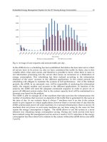
Table 27.16 and Figure 27.7 contain models listed in
ASHRAE’s Guideline 14-2002, which include steady-
state constant or mean models, models adjusted for the
days in the billing period, two-parameter models, three-
parameter models or variable-based degree-day models,
four-parameter models, five-parameter models, and
multivariate models. All of these models can be calcu-
lated with ASHRAE Inverse Model Toolkit (IMT), which
was developed from Research Project 1050-RP.
141
The steady-state, linear, change-point linear, vari-
able-based degree-day and multivariate inverse models
contained in ASHRAE’s IMT have advantages over
other types of models. First, since the models are simple,
and their use with a given dataset requires no human
intervention, the application of the models can be on can
be automated and applied to large numbers of build-
Table 27.16: Sample Models for the Whole-Building Approach from ASHRAE Guideline 14-2002.
152
736 ENERGY MANAGEMENT HANDBOOK
ings, such as those contained in utility databases. Such
a procedure can assist a utility, or an owner of a large
number of buildings, identify which buildings have
abnormally high energy use. Second, several studies
have shown that linear and change-point linear model
coeffi cients have physical signifi cance to operation of
heating and cooling equipment that is controlled by a

thermostat.
142,143,144,145
Finally, numerous studies have
reported the successful use of these models on a variety
of different buildings.
146,147,148,149,150,151
Steady-state models have disadvantages, includ-
ing: an insensitivity to dynamic effects (e.g., thermal
mass), insensitivity to variables other than temperature
(e.g., humidity and solar), and inappropriateness for
certain building types, for example building that have
strong on/off schedule dependent loads, or buildings
that display multiple change-points. If whole-building
models are required in such applications, alternative
models will need to be developed.
A. One-parameter or Constant Model
One-parameter, or constant models are models
where the energy use is constant over a given period.
Such models are appropriate for modeling buildings
that consume electricity in a way that is independent
of the outside weather conditions. For example, such
models are appropriate for modeling electricity use in
buildings which are on district heating and cooling sys-
tems, since the electricity use can be well represented by
a constant weekday-weekend model. Constant models
are often used to model sub-metered data on lighting
use that is controlled by a predictable schedule.
B. Day-adjusted Model
Day-adjusted models are similar to one-parameter
constant models, with the exception that the fi nal coef-

fi cient of the model is expressed as an energy use per
day, which is then multiplied by the number of days in
the billing period to adjust for variations in the utility
billing cycle. Such day-adjusted models are often used
with one, two, three, four and fi ve-parameter linear or
change-point linear monthly utility models, where the
energy use per period is divided by the days in the
billing period before the linear or change-point linear
regression is performed.
C. Two-parameter Model
Two-parameter models are appropriate for model-
ing building heating or cooling energy use in extreme
climates where a building is exposed to heating or
cooling year-around, and the building has an HVAC
system with constant controls that operates continu-
ously. Examples include outside air pre-heating systems
in arctic conditions, or outside air pre-cooling systems
in near-tropical climates. Dual-duct, single-fan, constant-
volume systems, without economizers can also be mod-
eled with two-parameter regression models. Constant
use, domestic water heating loads can also be modeled
with two-parameter models, which are based on the
water supply temperature.
D. Three-parameter Model
Three-parameter models, which include change-
point linear models or variable-based, degree day
Figure 27.7: Sample Models for the Whole-building
Approach. Included in this fi gure is: (a) mean or one-
parameter model, (b) two-parameter model, (c) three-
parameter heating model (similar to a variable based

degree-day model (VBDD) for heating), (d) three-pa-
rameter cooling model (VBDD for cooling), (e) four-
parameter heating model, (f) four-parameter cooling
model, and (g) fi ve-parameter model.
153
MEASUREMENT AND VERIFICATION OF ENERGY SAVINGS 737
models, can be used on a wide range of building types,
including residential heating and cooling loads, small
commercial buildings, and models that describe the gas
used by boiler thermal plants that serve one or more
buildings. In Table 27.16, three-parameter models have
several formats, depending upon whether or not the
model is a variable based degree-day model or three-
parameter, change-point linear models for heating or
cooling. The variable-based degree day model is defi ned
as:
E = C + B
1
(DD
BT
)
where
C = the constant energy use below (or above)
the change point, and
B
1
= the coeffi cient or slope that describes the
linear dependency on degree-days,
DD
BT

= the heating or cooling degree-days (or
degree hours), which are based on the
balance-point temperature.
The three-parameter change-point linear model for heat-
ing is described by
154
E = C + B
1
(B
2
– T)
+
where
C = the constant energy use above the
change point,
B
1
= the coeffi cient or slope that describes the
linear dependency on temperature,
B
2
= the heating change point temperature,
T = the ambient temperature for the period
corresponding to the energy use,
+ = positive values only inside the
parenthesis.
The three-parameter change-point linear model for cool-
ing is described by
E = C + B
1

(T – B
2
)
+
where
C = the constant energy use below the change
point,
B
1
= the coeffi cient or slope that describes the
linear dependency on temperature,
B
2
= the cooling change point temperature,
T = the ambient temperature for the period
corresponding to the energy use,
+ = positive values only for the parenthetical
expression.
E. Four-parameter Model
The four-parameter change-point linear heating
model is typically applicable to heating usage in build-
ings with HVAC systems that have variable-air volume,
or whose output varies with the ambient temperature.
Four-parameter models have also been shown to be
useful for modeling the whole-building electricity use
of grocery stores that have large refrigeration loads,
and signifi cant cooling loads during the cooling season.
Two types of four-parameter models are listed in Table
27.16, including a heating model and a cooling model.
The four-parameter change-point linear heating model

is given by
E = C + B
1
(B
3
- T)
+
- B
2
(T - B
3
)
+
where
C = the energy use at the change point,
B
1
= the coeffi cient or slope that describes the
linear dependency on temperature below
the change point,
B
2
= the coeffi cient or slope that describes the
linear dependency on temperature above
the change point
B
3
= the change-point temperature,
T = the temperature for the period of interest,
+ = positive values only for the parenthetical

expression.
The four-parameter change-point linear cooling model
is given by
E = C - B
1
(B
3
- T)
+
+ B
2
(T - B
3
)
+
where
C = the energy use at the change point,
B
1
= the coeffi cient or slope that describes
the linear dependency on temperature
below the change point,
B
2
= the coeffi cient or slope that describes
the linear dependency on temperature
above the change point
B
3
= the change-point temperature,

T = the temperature for the period of
interest,
+ = positive values only for the
parenthetical expression.
F. Five-parameter Model
Five-parameter change-point linear models are
useful for modeling the whole-building energy use
in buildings that contain air conditioning and electric
heating. Such models are also useful for modeling the
738 ENERGY MANAGEMENT HANDBOOK
weather dependent performance of the electricity con-
sumption of variable air volume air-handling units. The
basic form for the weather dependency of either case
is shown in Figure 27.7f, where there is an increase in
electricity use below the change point associated with
heating, an increase in the energy use above the change
point associated with cooling, and constant energy use
between the heating and cooling change points. Five-
parameter change-point linear models can be described
using variable-based degree day models, or a fi ve-pa-
rameter model. The equation for describing the energy
use with variable-based degree days is
E = C - B
1
(DD
TH
) + B
2
(DD
TC

)
where
C = the constant energy use between the
heating and cooling change points,
B
1
= the coeffi cient or slope that describes the
linear dependency on heating degree-days,
B
2
= the coeffi cient or slope that describes the
linear dependency on cooling degree-days,
DD
TH
= the heating degree-days (or degree hours),
which are based on the balance-point
temperature.
DD
TC
= the cooling degree-days (or degree hours),
which are based on the balance-point
temperature.
The fi ve-parameter change-point linear model that is
based on temperature is
E = C + B
1
(B
3
- T)
+

+ B
2
(T – B
4
)
+
where
C = the energy use between the heating and
cooling change points,
B
1
= the coeffi cient or slope that describes the
linear dependency on temperature below
the heating change point,
B
2
= the coeffi cient or slope that describes the
linear dependency on temperature above
the cooling change point
B
3
= the heating change-point temperature,
B
4
= the cooling change-point temperature,
T = the temperature for the period of interest,
+ = positive values only for the parenthetical
expression.
G. Whole-building Peak Demand Models
Whole-building peak electric demand models dif-

fer from whole-building energy use models in several
respects. First, the models are not adjusted for the days
in the billing period since the model is meant to repre-
sent the peak electric demand. Second, the models are
usually analyzed against the maximum ambient temper-
ature during the billing period. Models for whole-build-
ing peak electric demand can be classifi ed according to
weather-dependent and weather-independent models.
G-1. Weather-dependent
Whole-building Peak Demand Models
Weather-dependent, whole-building peak demand
models can be used to model the peak electricity use of
a facility. Such models can be calculated with linear and
change-point linear models regressed against maximum
temperatures for the billing period, or calculated with an
inverse bin model.
155,156
G-2. Weather-independent
Whole-building Peak Demand Models
Weather-independent, whole-building peak de-
mand models are used to measure the peak electric use
in buildings or sub-metered data that do not show sig-
nifi cant weather dependencies. ASHRAE has developed
a diversity factor toolkit for calculating weather-inde-
pendent whole-building peak demand models as part
of Research Project 1093-RP. This toolkit calculates the
24-hour diversity factors using a quartile analysis. An
example of the application of this approach is given in
the following section.
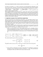
Example: Whole-building energy use models

Figure 27.8 presents an example of the typical data
requirements for a whole-building analysis, including
one year of daily average ambient temperatures and
twelve months of utility billing data. In this example
of a residence, the daily average ambient temperatures
were obtained from the National Weather Service (i.e.,
the average of the published min/max data), and the
utility bill readings represent the actual readings from
the customer’s utility bill. To analyze these data several
calculations need to be performed. First, the monthly
electricity use (kWh/month) needs to be divided by the
days in the billing period to obtain the average daily
electricity use for that month (kWh/day). Second, the
average daily temperatures need to be calculated from
the published NWS min/max data. From these average
daily temperatures the average billing period tempera-
ture need to be calculated for each monthly utility bill.
The data set containing average billing period tem-
peratures and average daily electricity use is then ana-
lyzed with ASHRAE’s Inverse Model Toolkit (IMT)
157
to
determine a weather normalized consumption as shown
MEASUREMENT AND VERIFICATION OF ENERGY SAVINGS 739
in Figures 27.9 and 27.10. In Figure 27.9 the twelve
monthly utility bills (kWh/period) are shown plotted
against the average billing period temperature along
with a three-parameter change-point model calculated
with the IMT. In Figure 27.10 the twelve monthly utility
bills, which were adjusted for days in the billing period

(i.e., kWh/day) are shown plotted against the average
billing period temperature along with a three-param-
eter change-point model calculated with the IMT. In
the analysis for this house, the use of an average daily
model improved the accuracy of the unadjusted model
(i.e., Figure 27.9) from an R
2
of 0.78 and CV (RMSE) of
24.0% to an R
2
of 0.83 and a CV (RMSE) of 19.5% for
the adjusted model (i.e., Figure 27.10), which indicates
a signifi cant improvement in the model.
In another example the hourly steam use (Figure
27.11) and hourly electricity use (Figure 27.13) for the
U.S. DOE Forrestal Building is modeled with a daily
weekday-weekend three-parameter, change-point model
for the steam use (Figure 27.12), and an hourly weekday-
weekend demand model for the electricity use (Figure
27.14). To develop the weather-normalized model for the
steam use the hourly steam data and hourly weather
data were fi rst converted into average daily data, then a
three-parameter, weekday-weekend model was calculat-
ed using the EModel software,
158
which contains similar
algorithms as ASHRAE’s IMT. The resultant model,
which is shown in Figure 27.12 along with the daily
steam, is well described with an R
2

of 0.87 an RMSE of
50,085.95 kBtu/day and a CV (RMSE) of 37.1%.
In Figure 27.14 hourly weather-independent 24-
hour weekday-weekend profi les have been created for
Figure 27.8: Example Data for Monthly Whole-building Analysis (upper trace, daily average temperature, F,
lower points, monthly electricity use, kWh/day).
Figure 27.9 Example Unadjusted Monthly Whole-
building Analysis (3P Model) for kWh/period (R
2
=
0.78, CV (RMSE) = 24.0%).
Figure 27.10. Example Adjusted Whole-building Anal-
ysis (3P Model) for kWh/day (R
2
= 0.83, CV (RMSE)
= 19.5%).
740 ENERGY MANAGEMENT HANDBOOK
the whole-building electricity use using ASHRAE’s
1093-RP Diversity Factor Toolkit.
159
These profi les can
be used to calculate the baseline whole-building electric-
ity use (i.e., using the mean hourly use) by multiplying
times the expected weekdays and weekends in the year.
The profi les can also be used to calculate the peak elec-
tricity use (i.e., using the 90th percentile).
Calculation of Annual Energy Use
Once the appropriate whole-building model has
been chosen and applied to the baseline data, the annual
energy use for the baseline period and the post-retrofi t

period are then calculated. Savings are then calculated
by comparing the annual energy use of the baseline with
the annual energy use of the post-retrofi t period.
Whole-building Calibrated Simulation Approach
Whole-building calibrated simulation normally
requires the hourly simulation of an entire building,
including the thermal envelope, interior and occupant
loads, secondary HVAC systems (i.e., air handling
units), and the primary HVAC systems (i.e., chillers,
boilers). This is usually accomplished with a general
purpose simulation program such as BLAST, DOE-2
or EnergyPlus, or similar proprietary programs. Such
programs require an hourly weather input file for
the location in which the building is being simulated.
Calibrating the simulation refers to the process whereby
selected outputs from the simulation are compared and
eventually matched with measurements taken from an
actual building. A number of papers in the literature
have addressed techniques for accomplishing these cali-
brations, and include results from case study buildings
where calibrated simulations have been developed for
various purposes.
160, 161, 162, 163, 164, 165, 166, 167, 168, 169,
170, 171,172,173,174,175
Applications of Calibrated Whole-building Simulation.
Calibrated whole-building simulation can be a
useful approach for measuring the savings from energy
conservation retrofi ts to buildings. However, it is gener-
ally more expensive than other methods, and therefore it
is best reserved for applications where other, less costly

approaches cannot be used. For example, calibrated
simulation is useful in projects where either pre-retrofi t
or post-retrofi t whole-building metered electrical data
are not available (i.e., new buildings or buildings with-
out meters such as many college campuses with central
facilities). Calibrated simulation is desired in projects
where there are signifi cant interactions between retrofi ts,
for example lighting retrofi ts combined with changes
to HVAC systems, or chiller retrofi ts. In such cases the
whole-building simulation program can account for
the interactions, and in certain cases, actually isolate
interactions to allow for end-use energy allocations. It
is useful in projects where there are signifi cant changes
in the facility’s energy use during or after a retrofi t has
been installed, where it may be necessary to account
for additions to a building that add or subtract thermal
loads from the HVAC system. In other cases, demand
may change over time, where the changes are not re-
lated to the energy conservation measures. Therefore,
adjustments to account for these changes will be also
be needed. Finally, in many newer buildings, as-built
design simulations are being delivered as a part of the
building’s fi nal documents. In cases where such simula-
tions are properly documented they can be calibrated to
the baseline conditions and then used to calculate and
measure retrofi t savings.
Unfortunately, calibrated, whole-building simula-
tion is not useful in all buildings. For example, if a
building cannot be readily simulated with available sim-
ulation programs, signifi cant costs may be incurred in

Figure 27.11: Example Heating Data for Daily Whole-building Analysis.
MEASUREMENT AND VERIFICATION OF ENERGY SAVINGS 741
modifying a program or developing a new program to
simulate only one building (e.g., atriums, underground
buildings, buildings with complex HVAC systems
that are not included in a simulation program’s sys-
tem library). Additional information about calibrated,
whole-building simulation can be found in ASHRAE’s
Guideline 14-2002.
Figure 27.15 provides an example of the use of
calibrated simulation to measure retrofi t savings in a
project where pre-retrofi t measurements were not avail-
Figure 27.12: Example
Daily Weekday-week-
end Whole-building
Analysis (3P Model)
for Steam Use (kBtu/
day, R
2
= 0.87, RMSE =
50,085.95, CV (RMSE)
= 37.1%). Weekday use
(x), weekend use ( ).
Figure 27.13: Example Electricity Data for Hourly Whole-building Demand Analysis.
Figure 27.14: Example Weekday-weekend Hourly Whole-building Demand Analysis (1093-RP Model) for Elec-
tricity Use.
742 ENERGY MANAGEMENT HANDBOOK
able. In this fi gure both the before-after whole-building
approach and the calibrated simulation approach are
illustrated. On the left side of the fi gure the traditional

whole-building, before-after approach is shown for a
building that had a dual-duct, constant volume system
(DDCV) replaced with a variable air volume (VAV) sys-
tem. In such a case where baseline data are available,
the energy use for the building is regressed against the
coincident weather conditions to obtain the representa-
tive baseline regression coeffi cients. After the retrofi t is
installed, the energy savings are calculated by compar-
ing the projected pre-retrofit energy use against the
measured post-retrofi t energy use, where the projected
pre-retrofi t energy use calculated with the regression
model (or empirical model), which was determined with
the facility’s baseline DDCV data.
In cases where the baseline data are not available
(i.e., the right side of the fi gure), a simulation of the
building can be developed and calibrated to the post-
retrofi t conditions (i.e., the VAV system). Then, using the
calibrated simulation program, the pre-retrofi t energy
use (i.e., DDCV system) can be calculated for conditions
in the post-retrofi t period, and the savings calculated by
comparing the simulated pre-retrofi t energy use against
the measured post-retrofi t energy use. In such a case
the calibrated post-retrofi t simulation can also be used
to fi ll-in any missing post-retrofi t energy use, which is
a common occurrence in projects that measure hourly
energy and environmental conditions. The accuracy of
the post-retrofi t model depends on numerous factors.
Methodology for Calibrated Whole-building Simulation
Calibrated simulation requires a systematic ap-
proach that includes the development of the whole-

building simulation model, collection of data from the
building being retrofi tted and the coincident weather
data. The calibration process then involves the com-
parison of selected simulation outputs against measured
data from the systems being simulated, and the adjust-
ment of the simulation model to improve the compari-
son of the simulated output against the corresponding
measurements. The choice of simulation program is
a critical step in the process, which must balance the
model appropriateness, algorithmic complexity, user
expertise, and degree of accuracy against the resources
available to perform the modeling.
Data collection from the building includes the col-
lection of data from the baseline and post-retrofi t peri-
ods, which can cover several years of time. Building data
to be gathered includes such information as the building
location, building geometry, materials characteristics,
equipment nameplate data, operations schedules, tem-
perature settings, and at a minimum whole-building
utility billing data. If the budget allows, hourly whole-
Figure 27.15: Flow Diagram for Calibrated Simulation Analysis of Air-Side HVAC System.
176
MEASUREMENT AND VERIFICATION OF ENERGY SAVINGS 743
building energy use and environmental data can be
gathered to improve the calibration process, which can
be done over short-term, or long-term period.
Figure 27.16 provides an illustration of a calibra-
tion process that used hourly graphical and statistical
comparisons of the simulated versus measured energy
use and environmental conditions. In this example, the

site-specifi c information was gathered and used to de-
velop a simulation input fi le, including the use of mea-
sured weather data, which was then used by the DOE-2
program to simulate the case study building. Hourly
data from the simulation program was then extracted
and used in a series of special-purpose graphical plots
to help guide the calibration process (i.e., time series, bin
and 3-D plots). After changes were made to the input
fi le, DOE-2 was then run again, and the output com-
pared against the measured data for a specifi c period.
This process was then repeated until the desired level of
calibration was reached, at which point the simulation
was proclaimed to be “calibrated.” The calibrated model
was then used to evaluate how the new building was
performing compared to the design intent.
A number of different calibration tools have been
reported by various investigators, ranging from simple
X-Y scatter plots to more elaborate statistical plots and
indices. Figures 27.17, 27.18 and 27.19 provide examples
of several of these calibration tools. In Figure 27.17 an
example of an architectural rendering tool is shown that
assists the simulator with viewing the exact placement
of surfaces in the building, as well as shading from
nearby buildings, and north-south orientation. In Figure
27.18 temperature binned calibration plots are shown
comparing the weather dependency of an hourly simu-
lation against measured data. In this fi gure the upper
plots show the data as scatter plots against temperature.
The lower plots are statistical, temperature-binned box-
whisker-mean plots, which include the super position-

ing of measured mean line onto the simulated mean line
to facilitate a detailed evaluation. In Figure 27.19 com-
parative three-dimensional plots are shown that show
measured data (top plot), simulated data (second plot
from the top), simulated minus measured data (second
plot from the bottom, and measured minus simulated
data (bottom plot). In these plots the day-of-the-year is
the scale across the page (y axis), the hour-of-the-day is
the scale projecting into the page (x axis), and the hourly
Figure 27.16: Calibration Flowchart. This fi gure shows
the sequence of processing routines that were used to
develop graphical calibration procedures.
178
Figure 27.17: Example Architecture Rendering of the
Robert E. Johnson Building, Austin, Texas.
179,180
744 ENERGY MANAGEMENT HANDBOOK
electricity use is the vertical scale of the surface above
the x-y plane. These plots are useful for determining
how well the hourly schedules of the simulation match
the schedules of the real building, and can be used to
identify other certain schedule-related features. For ex-
ample, in the front of plot (b) the saw-toothed feature
is indicating on/off cycling of the HVAC system, which
is not occurring in the actual building.
Table 27.17 contains a summary of the proce-
dures used for developing a calibrated, whole-building
simulation program, as defi ned in ASHRAE’s Guideline
14-2002. In general, to develop a calibrated simulation,
detailed information is required for a building, includ-

ing information about the building’s thermal envelope
(i.e., the walls, windows, roof, etc.), information about
the building’s operation, including temperature settings,
HVAC systems, and heating-cooling equipment that ex-
isted both during the baseline and post-retrofi t period.
This information is input into two simulation fi les, one
for the baseline and one for the post-retrofi t conditions.
Savings are then calculated by comparing the two
simulations of the same building, one that represents the
baseline building, and one that represents the building’s
operations during the post-retrofi t period.
27.2.2 Role of M&V
Each Energy Conservation Measure (ECM) pres-
ents particular requirements. These can be grouped in
functional sections as shown in Table 27.18. Unfortu-
nately, in most projects, numerous variables exist so
the assessments can be easily disputed. In general, the
low risk (L)—reasonable payback ECMs exhibit steady
performance characteristics that tend not to degrade
or become easily noticed when savings degradation
occurs. These include lighting, constant speed motors,
two-speed motors and IR radiant heating. The high
risk (H)—reasonable payback ECMs include EMCSs,
variable speed drives and control retrofi ts. The savings
from these ECMs can be overridden by building op-
erators and not be noticed until years later. Most other
ECMs fall in the category of “it depends.” The attention
that the operations and maintenance directs at these
dramatically impacts the sustainability of the operation
and the savings. With an EMCS, operators can set up

trend reports to measure and track occupancy schedule
overrides, the various reset schedule overrides, variable
speed drive controls and even monitor critical param-
eters which track mechanical systems performance. il-
lustrates a “most likely” range of ratings for the various
categories.
183
Often, building envelope or mechanical systems
need to be replaced. Building systems have fi nite life-
Figure 27.18: Temperature Bin Calibration Plots. This fi g-
ure shows the measured and simulated hourly weekday
data as scatter plots against temperature in the upper plots
and as statistical binned box-whisker-mean plots in the
lower plots.
181
Figure 27.19: Comparative Three-dimen-
sional Plots. (a) Measured Data. (b) Simu-
lated Data. (c) Simulated-Measured Data.
(d) Measured-Simulated Data.
MEASUREMENT AND VERIFICATION OF ENERGY SAVINGS 745
times, ranging from two to fi ve years for most light bulbs
to 10 to 20+ years for chillers and boilers. Building enve-
lope replacements like insulation, siding, roof, windows
and doors can have lifetimes from 10 to 50 years. In these
instances, life cycle costing should be done to compare
the total cost of upgrading to more effi cient technology.
Also, the cost of M&V should be considered when deter-
mining how to sustain the savings and performance of
the replacement. In many cases, the upgraded effi ciency
will have a payback of less than 10 years when compared

to the current effi ciency of the existing equipment. Cur-
rent technology high effi ciency upgrades normally use
controls to acquire the high efficiency. These controls
often connect to standard interfaces so that they commu-
nicate with today’s state of the art Energy Management
and Control Systems (EMCSs).
27.2.3 Cost/Benefi t Analysis
The target for work for the USAF has been 5%
of the savings.
184
The cost of the M&V can exceed 5%
if the risk of losing savings exceeds predefi ned limits.
The Variable Speed Drive ECM illustrates these op-
portunities and risks. VSD equipment exhibits high
reliability. Equipment type of failures normally happen
when connection breaks occur with the control input,
the remote sensor. Operator induced failures occur then
the operator sets the unit to 100% speed and does not
re-enable the control. Setting the unit to 100% can occur
for legitimate reasons. These reasons include running a
test, overriding a control program that does not provide
adequate speed under specifi c, and typically unusual,
circumstances, or requiring 100% operation for a limited
time. The savings disappear if the VSD remains at 100%
operating speed.
For example, consider a VSD ECM with ten (10)
motors with each motor on a different air handling
unit. Each motor has fi fty (50) horsepower (HP). The
base case measured these motors running 8760 hours
per year at full speed. Assume that the loads on the

motors matched the nameplate 50 HP at peak loads.
Table 27.17: Calibrated, whole-building Simulation Procedures from ASHRAE Guideline 14-2002.
177
746 ENERGY MANAGEMENT HANDBOOK
Although the actual load on a AHU fan varies with
the state of the terminal boxes, assume that the load
average equates to 80% of the full load since the duct
pressure will rise as the terminal boxes reduce fl ow at
the higher speed. Table 27.19 contains the remaining
assumptions. To correctly determine the average power
load, the average power must either be integrated over
the period of consumption or the bin method must be
used. For the purposes of this example, the 14.4% value
will be used.
The equation below shows the relationship be-
tween the fan speed and the power consumed. The ex-
ponent has been observed to vary between 2.8 (at high
fl ow) and 2.7 (at reduced fl ow) for most duct systems.
This includes the loss term from pressure increases at
a given fan speed. Changing the exponent from 2.8 to
2.7 reduces the savings by less than 5%.

Pwr = Pwr
0
×
% Speed
Full Speed
2.8
Demand savings will not be considered in this ex-
ample. Demand savings will likely be very low if the util-

ity has a 12-month ratchet clause and the summer load
requires some full speed operation during peak times.
Assuming a $12.00/kW per month demand charge, de-
mand savings could be high for off-season months if the
demand billing resets monthly. Without a ratchet clause,
rough estimates have yearly demand savings ranging up
to $17,000 if the fan speed stays under 70% for 6 months
per year. Yearly demand savings jump to over $20,000 if
the fan speed stays under 60% for 6 months per year.
Table 27.18: Overview of Risks and Costs for ECMs.
Table 27.19: VSD Example Assumptions.
MEASUREMENT AND VERIFICATION OF ENERGY SAVINGS 747
Figure 27.20 illustrates the savings expected from
the VSD ECM by hours of use per year. The 5% and
10% of Savings lines defi ne the amount available for
M&V expenditures at these levels. In this example, the
ECM savings exceeds $253,000 per year. Five percent
(5%) of savings over a 20-year project life makes $253K
available for M&V and ten percent (10%) of the sav-
ings makes $506K available over the 20-year period. If
the motors run less frequently than continuous, savings
decrease as shown in Figure 27.20. Setting up the M&V
program to monitor the VSDs on an hourly basis and
report savings on a monthly report requires monitoring
the VSD inverter with an EMCS to poll the data and
create reports.
To provide the impact of the potential losses from
losing the savings, assume the savings degrades at a
loss of 10% of the total yearly savings per year. Studies
have shown that control ECMs like the VSD example

can expect to see 20% to 30% degradation in savings in
2 to 3 years. Figure 27.21 illustrates what happens to the
savings in 20 years with 10% of the savings spent on
M&V. Note that the losses exceed the M&V cost during
the fi rst year, resulting in a net loss of almost $3,000,000
over the 20-year period. Figure 27.22 shows the savings
per year with a 10% loss of savings. M&V costs remain
at 10% of savings. At the end of the 20-year period, the
savings drop to almost $30,000 per year out of a poten-
tial savings of over $250,000 per year.
This example shows the cumulative impact of los-
ing savings on a year by year basis. The actual savings
amounts will vary depending upon the specifi c factors
in an ECM and can be scaled to refl ect a specifi c applica-
tion. Increasing the M&V cost to reduce the loss of sav-
ings often makes sense and must be carefully thought
through.
27.2.4 Cost Reduction Strategies
M&V strategies can be cost reduced by lowering
the requirements for M&V or by statistical sampling.
Reducing requirements involves performing trade-offs
with the risks and benefi ts of having reliable numbers to
determine the savings and the costs for these measure-
ments.
27.2.4.1 Constant Load ECMs
Lighting ECMs can save 30% of the pre-ECM
energy and have a payback in the range of 3 to 6
years. Assuming that the lighting ECM was designed
and implemented per the specifi cations and the sav-
ings were verifi ed to be occurring, just verifying that

the storeroom has the correct ballasts and lamps may
constitute acceptable M&V on a yearly basis. This costs
far less than performing a yearly set of measurements,
analyzing them and then creating reports. In this case,
other safeguards should be implemented to assure that
the bulb and ballast replacement occurs and meets the
Figure 27.20: Example VSD EMC Yearly Savings/M&V
Cost.
Figure 27.21: Yearly Impact of Ongoing Losses. Figure 27.22: Cumulative Impact of Savings Loss.
748 ENERGY MANAGEMENT HANDBOOK
requirements specifi ed.
High effi ciency motor replacements provide an-
other example of constant load ECMs. The key short
term risks with motor replacements involve installing
the right motor with all mechanical linkages and elec-
trical components installed correctly. Once verifi ed, the
long term risks for maintaining savings occur when the
motor fails. The replacement motor must be the correct
motor or savings can be lost. A sampled inspection re-
duces this risk. Make sure to inspect all motors at least
once every fi ve (5) years.
27.2.4.2 Major Mechanical Systems
Boilers, chillers, air handler units, cooling towers
comprise the category of manor mechanical equipment
in buildings. They need to be considered separately as
each carry their own set of short-term and long-term
risks. In general, measurements provide necessary
risk reduction. The question becomes: What measure-
ments reduce the risk of savings loss by an acceptable
amount?

First a risk assessment needs to be performed. The
short-term risks for boilers involve installing the wrong
size or installing the boiler improperly (not to specifi -
cations). Long-term savings sustainability risks tend to
focus on the water side and the fi re side. Water deposits
(K
+
, Ca
++
, Mg
+
) will form on the inside of the tubes and
add a thermal barrier to the heat fl ow. The fi re side can
add a layer of soot if the O
2
level drops too low. Either
of these reduce the effi ciency of the boiler over the long
haul. Generally this can take several years to impact
the effi ciency if regular tune-ups and water treatment
occurs.
Boilers come in a wide variety of shapes and
sizes. Boiler size can be used as a defi ning criterion for
measurements. Assume that natural gas or other boiler
fuels cost about $5.00 per MMBtu. Although fuel price
constantly changes, it provides a reference point for this
analysis. Thus a boiler with 1MMBtu per hour output,
an effi ciency of 80% and operating at 50% load 3500
hours per year, consumes about $11,000 per year. If this
boiler replaced a less effi cient boiler, say at 65%, then the
net savings amounts to about $2,500 per year, assuming

the same load from the building. At 5% of the savings,
$125 per year can be used for M&V. This does not al-
low much M&V. At 10% of the annual savings, $250 per
year can be used. At this level of cost, a combustion ef-
fi ciency measurement could be performed, either yearly
or bi-yearly, depending on the local costs. In 2003 the
ASME’s Power Test Code 4.1 (PTC-4.1)
185
was replaced
with PTC4. Either of these codes allows two methods
to measuring boiler effi ciency. The fi rst method uses
the energy in equals energy out—using the fi rst law of
thermodynamics. This requires measuring the Btu input
via the gas fl ow and the Btu output via the steam (or
water) fl ow and temperatures. The second method mea-
sures the energy loss due to the content and tempera-
ture of the exhausted gases, radiated energy from the
shell and piping and other loss terms (like blowdown).
The energy loss method can be performed in less than
a couple of hours. The technician performing these
measurements must be skilled or signifi cant errors will
result in the calculated effi ciency. The equation below
shows the calculations required.
Effi ciency = 100% – Losses + Credits
The losses term includes the temperature of the
exhaust gas and a measure of the unburned hydrocar-
bons by measuring CO
2
or O
2

levels, the loss due to
excess CO and a radiated term. Credits seldom occur
but could arise from sola r heating t he makeup water
or s imilar contributions. The Greek letter “η” us ually
denotes effi ciency.
As with boilers, a risk assessment needs to be
performed for chilers. The short term risks for chillers
involve sizing or improper installation. Long term sav-
ings sustainability risks focus on the condenser water
system, as circulation occurs in an open system. Water
deposits (K
+
, Ca
++
, Mg
+
, organics) will form on the
inside of the condenser tubes and add a barrier to the
thermal fl ow. These reduce the effi ciency of the chiller
over the long haul. Generally this can take several years
to impact the effi ciency if proper water treatment occurs.
Depending on the environmental conditions, the quality
of the makeup water and the water treatment, condenser
tube fouling should be checked every year or at least
every other year.
Chillers consume electricity in the case of most
centrifugal, screw, scroll and reciprocating compressors.
Direct-fi red absorbers and engine driven compressors
use a petroleum based fuel. As with boilers, chiller
size and application sets the basic energy consumption

levels. Assume, for the purpose of this example, that
electricity provides the chiller energy. Older chillers with
water towers often operate at the 0.8 to 1.3 kW per ton
level of effi ciency. New chillers with water towers can
operate in the 0.55 to 0.7 range of effi ciency. Note that
the effi ciency of any chiller depends upon the specifi c
operating conditions. Also assume the following: 500
Tons centrifugal chiller with the specifi cations shown in
Table 27.20. Under these conditions the chiller produces
400 Tons of chilled water and requires an expenditure
of $ 38,000 per year, considering both energy use and
MEASUREMENT AND VERIFICATION OF ENERGY SAVINGS 749
demand charges. Some utilities only charge demand
charges on the transmission and delivery (T&D) parts
of the rate structure. In that case, the cost at $0.06/kWh
would be closer to $28,000. Using the 5% (10%) guide-
line for M&V costs as a percentage of savings leaves
almost $1,100 ($2,200) per year to spend on M&V. This
creates an allowable expenditure over a 20-year project
of $22,000 ($44,000) for M&V. If the utility has a ratchet
clause in the rate structure, the amount for M&V in-
creases to $1,700 ($3,400) per year. At $1,100 per year,
trade-offs will need to be made to stay within that
“budget.” The risks need to be weighed and decisions
made as to what level of M&V costs will be allowed.
To determine the actual effi ciency of a chiller re-
quires accurate measurements of the chilled water fl ow,
the difference between the chilled water supply and
return temperatures and the electrical power provided
to the chiller. Costs can be reduced using an EMCS if

only temperature, fl ow and power sensors need to be
installed.
sustainability risks. When an operator overrides a strat-
egy and forgets to re-enable it, the savings disappear. A
common EMCS ECM requires the installation of equip-
ment and programs used to set back temperatures or
turn off equipment. Short term risks involve setting up
the controls so that performance enhances, or at least
does not degrade, the comfort of the occupants. When
discomfort occurs, either occupants set up “portable
electric reheat units” or operators override the control
program. For example, when the night set-back control
does not get the space to comfort by occupancy, opera-
tors typically override instead of adjusting the param-
eters in the program. These actions tend to occur during
peak loading times and then not get re-enabled during
milder times. Long term risks cover the same area as
short term risks. A new operator or a failure in remote
equipment that does not get fi xed will likely cause the
loss of savings. Estimating the savings cost for various
projects can be done when the specifi cs are known.
Table 27.20: Example of Savings with a 500 Ton Chiller.
Table 27.21: Sampling Requirements.
Cooling tower replacement requires knowledge of
the risks and costs involved. As with boilers and chillers,
the primary risks involve the water treatment. Controls
can be used to improve the effi ciency of a chiller/tower
combination by as much as 15% to 20%. As has been
previously stated, control ECMs often get overridden
and the savings disappear.

27.2.4.3 Control Systems
Control ECMs encompass a wide spectrum of capa-
bilities and costs. Upgrading a pneumatic control system
and installing EP (electronic to pneumatic) transducers
involves the simple end. The complex side could span
installing a complete EMCS with sophisticated controls,
with various reset, pressurization and control strategies.
Generally, EMCSs function as basic controls and do not
get widely used in sophisticated applications.
Savings due to EMCS controls bear high
750 ENERGY MANAGEMENT HANDBOOK
Risk abatement can be as simple as requiring a
trend report weekly or at least monthly. M&V costs can
generally be easily held under 5% when using an EMCS
and creating trend reports.
27.2.5 M&V Sampling Strategies
M&V can be made signifi cantly lower cost by sam-
pling. Sampling also reduces the timeliness of obtain-
ing specifi c data on specifi c equipment. The benefi ts of
sampling arise when the population of items increases.
Table 27.21 (M&V Guidelines: Measurement and Verifi -
cation for Federal Energy Projects, Version 2.2, Appendix
D) illustrates how confi dence and precision impact the
number of samples required in a given population of
items.
Lighting ECMs may involve thousands of fi xtures.
For example, to obtain a savings estimate for 1,000 or
more fi xtures, with a confi dence of 80% and a precision
of 20%, 11 fi xtures would need to be sampled. If the
requirements increased to a confi dence of 90% and a pre-

cision of 10%, 68 fi xtures would need to be sampled.
The boiler ECM also represents opportunity for
M&V cost reduction using sampling. Assume that the
ECM included replacing 50 boilers. If a confi dence of
80% and a precision of 20% satisfy the requirements,
10 boilers would need to be sampled. The cost is then
reduced to 20% of the cost of measuring all boilers, a
signifi cant savings. A random sampling to select the
sample set can easily be implemented.
References
1. Claridge D.E., Turner, W.D., Liu, M., Deng, S., Wei, G., Culp, C.,
Chen, H., and Cho, S. 2002. “Is Commissioning Once Enough?”
Solutions for Energy Security and Facility Management Chal-
lenges: Proceedings of the 25th WEEC, Atlanta, GA, October
19-11, 2002, pp. 29-36.
2. Haberl, J., Lynn, B., Underwood, D., Reasoner, J., Rury, K. 2003.
“Development an M&V Plan and Baseline for the Ft. Hood
ESPC Project,” ASHRAE Seminar Presentation, (June).
3. C. Culp, K.Q. Hart, B. Turner, S. Berry-Lewis, 2003. “Energy
Consumption Baseline: Fairchild AFB’s Major Boiler Retrofi t,”
ASHRAE Seminar (January).
4. Arnold, D., 1999. “The Evolution of Modem Offi ce Buildings
and Air Conditioning,” ASHRAE Journal, American Society of
Heating Refrigeration Air-conditioning Engineers, Atlanta, GA,
pp. 40-54, (June).
5. Donaldson, B., Nagengast. 1994. Heat and Cold: Mastering
the Great Indoors. American Society of Heating Refrigeration
Air-conditioning Engineers, Atlanta, GA.
6. Cheney, M., Uth, R. 1999. Tesla: Master of Lightning. Barnes
and Noble Books, New York, N,Y.

7. Will, H. 1999. The First Century of Air Conditioning. American
Society of Heating Refrigeration Air-conditioning Engineers,
Atlanta, GA.
8. Israel, P. 1998. Edison: A Life of Invention. John Wiley and
Sons, New York, N.Y.
9. EEI 1981. Handbook for Electricity Metering, 8th Edition with
Appendix, Edition Electric Institute, Washington D.C.
10. Miller, R. 1989. Flow Measurement Engineering Handbook.
McGraw Hill, New York, N.Y.
11. American Institute of Physics, 1975. Effi cient Use of Energy:
The APS Studies on the Technical Aspects of the More Effi cient
Use of Energy, American Physical Society, New York, N.Y., (A
report on the 1973 summer study at Princeton University).
12. National Geographic, February 1981. Special Report on Energy:
Facing up to the Problem, Getting Down to Solutions, National
Geographic Society, Washington, D.C.
13. Scientifi c American 1971. Energy and Power. W.H. Freeman
and Company, San Francisco, CA. (A reprint of eleven articles
that appeared in the September 1971 Scientifi c American).
14. Kusuda, T. 1999. “Early History and Future Prospects of Build-
ing System Simulation,” Proceedings of the Sixth International
Building Performance Simulation Association (IBPSA BS’ 99),
Kyoto, Japan, (September).
15. APEC 1967. HCC-heating/cooling load calculations program.
Dayton, Ohio, Automated Procedures for Engineering Consul-
tants.
16. Ayres, M., Stamper, E. 1995. “Historical Development of Build-
ing Energy Calculations,” ASHRAE Transactions, Vol. 101, Pt.
1. American Society of Heating Refrigeration Air-conditioning
Engineers, Atlanta, GA.

17. Stephenson, D., and Mitalas, G. 1967. “Cooling Load Calcula-
tions by Thermal Response Factor Method,” ASHRAE Transac-
tions, Vol. 73, pt. 1.
18. Mitalas, G. and Stephenson, D. 1967, “Room Thermal Response
Factors,” ASHRAE Transactions, Vol. 73, pt. 2.
19. Stoecker, W. 1971. Proposed Procedures for Simulating the
Performance of Components and Systems for Energy Calcula-
tions, 2 “d Edition, American Society of Heating Refrigeration
Air-conditioning Engineers, Atlanta, GA.
20. Sepsy, C. 1969. “Energy Requirements for Heating, and Cooling
Buildings (ASHRAE RP 66-OS), Ohio State University.
21. Socolow, R. 1978. Saving Energy in the Home: Princeton’s
Experiments at Twin Rivers, Ballinger Publishing Company,
Cambridge, Massachusetts, (This book contains a collection of
papers that were also published in Energy and Buildings, Vol.
1, No. 3., (April)).
22. Fels, M. 1986. Special Issue Devoted to Measuring Energy Sav-
ings: The Scorekeeping Approach, Energy and Buildings, Vol.
9, Nos. 1 & 2, Elsevier Press, Lausanne, Switzerland, (Febru-
ary/May).
23. DOE 1985. Proceedings of the DOE/ORNL Data Acquisition
Workshop, Oak Ridge National Laboratory, Oak Ridge, TN,
(October).
24. Lyberg, M. 1987. Source Book for Energy Auditors: Vols. 1 &
2, International Energy Agency, Stockholm, Sweden, (Report
on IEA Task XI).
25. IEA 1990. Field Monitoring For a Purpose. International Energy
Agency Workshop, Chalmers University, Gothenburg, Sweden,
(April).
26. Oninicomp 1984. Faser Software, Omnicomp, Inc., State Col-

lege, PA, (monthly accounting software with VBDD capabil-
ity).
27. Eto, J. 1988. “On Using Degree-days to Account for the Effects
of Weather on Annual Energy Use in Offi ce Buildings,” Energy
and Buildings, Vol. 12, No. 2, pp. 113-127.
28. SRC Systems 1996. Metrix: Utility Accounting System, Berke-
ley, CA, (monthly accounting software with combined VBDD/
multiple regression capabilities).
29. Haberl, J. and Vajda. E. 1988. “Use of Metered Data Analysis
to Improve Building Operation and Maintenance: Early Results
From Two Federal Complexes,” Proceedings of the ACEEE
1988 Summer Study on Energy Efficient Buildings, Pacific
Grove, CA, pp. 3.98 - 3.111, (August).
30. Sonderegger, R. 1977. Dynamic Models of House Heating
Based on Equivalent Thermal Parameters, Ph.D. Thesis, Center
MEASUREMENT AND VERIFICATION OF ENERGY SAVINGS 751
for Energy and Environmental Studies, Report No. 57, Princ-
eton University.
31. DOE 1985. op.cit.
32. Lyberg, M. 1987. op.cit.
33. IEA 1990. op.cit.
34. ASHRAE 199 1. Handbook of HVAC Applications, Chapter
37: Building Energy Monitoring, American Society of Heating
Refrigeration Air-conditioning Engineers, Atlanta, GA.
35. Haberl, J., and Lopez, R. 1992. “LoanSTAR Monitoring Work-
book: Workbook and Software for Monitoring Energy in
Buildings,” submitted to the Texas Governor’s Energy Offi ce,
Energy Systems Laboratory, Texas A&M University, (August).
36. Claridge, D., Haberl, J., O’Neal, D., Heffi ngton, W., Turner, D.,
Tombari, C., Roberts, M., Jaeger, S. 1991. “Improving Energy

Conservation Retrofits with Measured Savings.” ASHRAE
Journal, Volume 33, Number 10, pp. 14-22, (October).
37. Fels, M., Kissock, K., Marean, M., and Reynolds, C. 1995.
PRISM, Advanced Version 1.0 User’s Guide, Center for Energy
and Envirom-nental Studies, Princeton University, Princeton,
N.J., (January).
38. ASHRAE 1999, I-IVACO 1 Toolkit: A Toolkit for Primary HVAC
System Energy Calculation, ASHRAE Research Project -RP 665,
Lebrun, J., Bourdouxhe, J-P, and Grodent, M., American Society
of Heating Refrigeration Air-conditioning Engineers, Atlanta,
GA.
39. ASHRAE 1993. HVAC02 Toolkit: Algorithms and Subroutines
for Secondary HVAC System Energy Calculations, ASHRAE
Research Project - 827-RP, Authors: Brandemuehl, M., Gabel,
S.,Andresen, American Society of Heating Refrigeration Air-
conditioning Engineers, Atlanta, GA.
40. Brandemuehl, M., Krarti, M., Phelan, J. 1996, “827-RP Final
Report: Methodology Development to Measure In-Situ Chiller,
Fan, and Pump Performance,” ASHRAE Research, ASHRAE,
Atlanta, GA, (March).
41. Haberl, J., Reddy, A., and Elleson, J. 2000a. “Determining Long-
Term performance Of Cool Storage Systems From Short-Term
Tests, Final Report,” submitted to ASHRAE under Research
Project 1004-RP, Energy Systems Laboratory Report ESL-TR-
00/08-01, Texas A&M University, 163 pages, (August).
42. Kissock, K., Haberl, J., and Claridge, D. 2001. “Development
of a Toolkit for Calculating Linear, Changepoint Linear and
Multiple-Linear Inverse Building Energy Analysis Models:
Final Report,” submitted to ASHRAE under Research Project
1050-RP, University of Dayton and Energy Systems Laboratory,

(December).
43. Abushakra, B., Haberl, J., Claridge, D., and Sreshthaputra, A.
2001 “Compilation Of Diversity Factors And Schedules For
Energy And Cooling Load Calculations; ASHRAE Research
Project 1093: Final Report,” submitted to ASHRAE under
Research Project 1093-RP, Energy Systems Lab Report ESL-TR-
00/06-01, Texas A&M University, 150 pages, (June).
44. MacDonald, J. and Wasserman, D. 1989. Investigation of
Metered Data Analysis Methods for Commercial and Related
Buildings, Oak Ridge National Laboratory Report No. ORNL/
CON-279, (May).
45. Rabl, A. 1988. “Parameter Estimation in Buildings: Methods for
Dynamic Analysis of Measured Energy Use,” Journal of Solar
Energy Engineering, Vol. 110, pp. 52-66.
46. Rabl, A., Riahle, A. 1992. “Energy Signature Model for Com-
mercial Buildings: Test With Measured Data and Interpreta-
tion,” Energy and Buildings, Vol. 19, pp. 143-154.
47. Gordon, J.M. and Ng, K.C. 1994. “Thermodynamic Modeling
of Reciprocating Chillers,” Journal of Applied Physics, Volume
75, No. 6, March 15, 1994, pp. 2769-2774.
48. Claridge, D.E., Haberl, J. S., Sparks, R., Lopez, R., Kissock,
K. 1992. “Monitored Conu-nercial Building Energy Data: Re-
porting the Results.” 1992 ASHRAE Transactions Symposium
Paper, Vol. 98, Part 1, pp. 636-652.
49. Sonderegger, R. 1977, op.cit.
50. Subbarao, K., Burch, J., Hancock, C.E, 1990. “How to accurately
measure the load coeffi cient of a residential building,” Journal
of Solar Energy Engineering, in preparation.
51. Reddy, A. 1989. “Application of Dynamic Building Inverse
Models to Three Occupied Residences Monitored Non-intru-

sively,” Proceedings of the Thermal Performance of Exterior
Envelopes of Buildings IV, ASHRAE/DOE/BTECC/CIBSE.
52. Shurcliff, W.A. 1984. “Frequency Method of Analyzing a
Building’s Dynamic Thermal Performance, W.A. Shurcliff, 19
Appleton St., Cambridge, MA.
53. Dhar, A. 1995, “Development of Fourier Series and Artifi cial
Neural Networks Approaches to Model Hourly Energy Use
in Commercial Buildings,” Ph.D. Dissertation, Mechanical
Engineering Department, Texas A&M University, May.
54. Miller, R., and Seem, J. 199 1. “Comparison of Artifi cial Neural
Networks with Traditional Methods of Predicting Return Time
from Night Setback,” ASHRAE Transactions, Vol. 97, Pt.2, pp.
500-508.
55. J.F. Kreider and X.A. Wang, (199 1). “Artifi cial Neural Net-
works Demonstration for Automated Generation of Energy
Use Predictors for Commercial Buildings.” ASHRAE Transac-
tions, Vol. 97, part 1.
56. Kreider, J. and Haberl, J. 1994. “Predicting Hourly Building
Energy Usage: The Great Energy Predictor Shootout: Overview
and Discussion of Results,” ASHRAE Transactions-Research,
Volume 100, Part 2, pp. 1104 - 1118, (June).
57. ASHRAE 1997. Handbook of Fundamentals, Chapter 30:
Energy Estimating and Modeling Methods, American Society
of Heating Refrigeration Air-conditioning Engineers, Atlanta,
GA., p. 30.27 (Copied with perinission).
58. ASHRAE 1997. op.cit., p. 30.28 (Copied with permission).
59. USDOE 1996. North American Energy Measurement and
Verifi cation Protocol (NEMVP), United States Department of
Energy DOE/EE-0081, (March).
60. FEMP 1996. Standard Procedures and Guidelines for Verifi -

cation of Energy Savings Obtained Under Federal Savings
Performance Contracting Programs, USDOE Federal Energy
Management Program (FEMP).
61. Haberl, J., Claridge, D., Turner, D., O’Neal, D., Heffi ngton, W.,
Verdict, M. 2002. “LoanSTAR After 11 Years: A Report on the
Successes and Lessons Learned From the LoanSTAR Program,”
Proceedings of the 2nd International Conference for Enhanced
Building Operation,” Richardson, Texas, pp. 131-138, (Octo-
ber).
62. USDOE 1997. International Performance Measurement and
Verifi cation Protocol (IPMVP), United States Department of
Energy DOE/EE-0157, (December).
63. USDOE 2001. International Performance Measurement and
Verifi cation Protocol (IPMVP): Volume 1: Concepts and Op-
tions for Determining Energy and Water Savings, United States
Department of Energy DOE/GO-102001-1187 (January).
64. USDOE 2001. International Performance Measurement and
Verification Protocol (IPMVP): Volume 11: Concepts and
Practices for Improved Indoor Environrnental Quality, United
States Department of Energy DOE/GO-102001-1188 (Janu-
ary).
65. USDOE 2003. International Performance Measurement and
Verification Protocol (IPMVP): Volume 11: Concepts and
Practices for Improved Indoor Environmental Quality, United
States Department of Energy DOE/GO-102001-1188 (Janu-
ary).
66. ASHRAE 2002.Guideline 14: Measurement of Energy and
Demand Savings, American Society of Heating Refrigeration
Air-conditioning Engineers, Atlanta, GA (September).
67. Hansen, S. 1993. Performance Contracting for Energy and Envi-

ronmental Systems, Fairmont Press, Lilbum, GA, pp. 99-100.
68. ASHRAE 2002. op.cit., pp. 27-30.
752 ENERGY MANAGEMENT HANDBOOK
69. lbid, p. 30 (Copied with permission).
70. Brandemuehl et al. 1996. op.cit.
71. Wei, G. 1997. “A Methodology for In-situ Calibration of Steam
Boiler Instrumentation,” MS Thesis, Mechanical Engineering
Department, Texas A&M University, August.
72. Dukelow, S.G. 1991. The Control of Boilers. Research Triangle
Park, NC: Instrument Society of America.
73. Dyer, F.D. and Maples, G. 1981. Boiler Effi ciency Improvement.
Boiler Effi ciency Institute. Auburn: AL.
74. Garcia-Borras, T. 1983. Manual for Improving Boiler and Fur-
nace Performance. Houston, TX: Gulf Publishing Company.
75. Aschner, F.S. 1977. Planning Fundamentals of Thermal Power
Plants. Jerusalem, Israel: Israel Universities Press.
76. ASME 1974 Performance Test for Steam Units — PTC 4. 1 a
1974.
77. Babcock and Wilcox. 1992. “Steam: Its generation and Use,”
Babcock and Wilcox, Barberton, Ohio, ISBN 0-9634570-0-4.
78. Katipamula, S., and Claridge, D. 1992. “Monitored Air Handler
Performance and Comparison with a Simplifi ed System Model,”
ASHRAE Transactions, Vol. 98, Pt 2., pp. 341-35 1.
79. Liu, M., and Claridge, D. 1995 “Application of Calibrated
HVAC Systems to Identify Component Malfunctions and to
Optimize the Operation and Control Schedules,” ASME/JSME
International Solar Energy Conference, pp. 209-217.
80. ASHRAE 2002. op.cit., p. 144.
81. Brandemuehl, et al. 1996. op. cit.
82. ASHRAE 2002, op cit., p. 144, (Copied with permission).

83. ASHRAE 2002. op.cit., pp. 144-147, (Copied with permis-
sion).
84. ASHRAE 2002. op.cit., p. 144.
85. Ibid, p. 148, (Copied with permission).
86. ASHRAE 2002. op.cit., pp. 147-149, (Copied with permis-
sion).
87. Gordon, J.M. and Ng, K.C. 1994. op.cit.
88. Gordon, J.M. and Ng, K.C., 1995. “Predictive and diagnostic
aspects of a universal thermodynamic model for chillers,”
International Journal of Heat Mass Transfer, 38(5), p.807.
89. Gordon, J.M., Ng, K.C., and Chua, H.T., 1995. “Centrifugal
chillers: thermodynamic modeling and a diagnostic case
study,” International Journal of Refrigeration, 18(4), p.253.
90. LBL. 1980. DOE-2 User Guide, Ver. 2. 1. Lawrence Berkeley
Laboratory and Los Alamos National Laboratory, Rpt No. LBL-
8689 Rev. 2; DOE-2 User Coordination Offi ce, LBL, Berkeley,
CA.
91. LBL. 198 1. DOE-2 Engineers Manual, Ver. 2. 1 A, Lawrence
Berkeley Laboratory and Los Alamos National Laboratory,
Rpt No. LBL-1 1353; DOE-2 User Coordination Offi ce, LBL,
Berkeley, CA.
92. LBL. 1982. DOE-2.1 Reference Manual Rev. 2.1A. Lawrence
Berkeley Laboratory and Los Alamos National Laboratory, Rpt
No. LBL-8706 Rev. 2; DOE-2 User Coordination Offi ce, LBL,
Berkeley, CA. LBL.
93. LBL. 1989. DOE-2 Supplement, Ver 2. 1 D. Lawrence Berkeley
Laboratory, Rpt No. LBL-8706 Rev. 5 Supplement. DOE-2 User
Coordination Offi ce, LBL, Berkeley, CA.
94. Haberl, J. S., Reddy, T. A., Figueroa, I., Medina, M. 1997. “Over-
view of LoanSTAR Chiller Monitoring and Analysis of In-Situ

Chiller Diagnostics Using ASHRAE RP827 Test Method,” Pro-
ceedings of the PG&E Cool Sense National Integrated Chiller
Retrofi t Forum (September).
95. According to Gordon et al. 1995, fHx is a dimensionless term
that is norrrially negligible.
96. Wei, G. 1997. op.cit.
97. Dukelow, S.G. 1991. op.cit.
9.8 Dyer, F.D. and Maples, G. 198 1. op.cit.
99. Garcia-Borras, T. 1983. op.cit.
100. Aschner, F.S. 1977. op.cit.
101. ASME 1974. op.cit.
102. Babcock and Wilcox. 1992. op.cit.
103. Haberl, J., Lynn, B., Underwood, D., Reasoner, J., Rury, K. 2003.
op.cit.
104. Haberl, et al. 2003. ibid.
105. ASME, 1974. Power Test Codes (PTC) 4. la, Steam Generating
Units. New York: ASME.
106. Stallard, G.S. and Jonas, T.S. 1996. Power Plant Engineering:
Combustion Processes. New York: Chapman & Hall.
107. Payne, F.W. 1985. Effi cient Boiler Operations Sourcebook. At-
lanta, GA: The Fairmont Press.
108. Wei 1997. op.cit.
109. Wei 1997. ibid.
110. Aschner 1977. op.cit.
111. Babcock and Wilcox 1992. op.cit.
112. Dukelow 1991. op.cit.
113. Witte, L.C., Schmidt, P.S., and Brown, DR. 1988. Industrial
Energy Management and Utilization. New York: Hemisphere
Publishing Corporation.
114. Aschner 1977. op.cit.

115. Thumann, A. 1988. Guide to Improving Effi ciency of Combus-
tion Systems. Lilburn, GA: The Fairmont Press.
116. Wei 1997. op.cit.
117. Garcia-Borras, T. 1983. Manual for Improving Boiler and Fur-
nace Performance. Houston, TX: Gulf Publishing Company.
118. Wei 1997. op.cit.
119. ASHRAE 2002, op.cit., pp. 154-156, (Copied with permis-
sion).
120. Bou Saada, T., Haberl, J., Vajda, J., and Harris, L. 1996. “Total
Utility Savings From the 37,000 Fixture Lighting Retrofi t to the
USDOE Forrestal Building,” Proceedings of the 1996 ACEEE
Summery Study, (August).
121. Abushakra, B., Sreshthaputra, A., Haberl, J., and Claridge, D.
2001. “Compilation of Diversity Factors and Schedules for En-
ergy and Cooling Load Calculations - Final Report,” submitted
to ASHRAE under Research Project 1093-RP, Energy Systems
Lab Report ESL-TR-01/04-01, Texas A&M University, (April).
122. IESNA 2003. Lighting Handbook, 9h Edition, Illuminating
Engineering Society of North America, New York, N.Y.
123. ASHRAE 2002, op.cit., pp. 156-159, (Copied with permis-
sion).
124. ASHRAE 2002, op. cit., p. 160, (Copied with permission).
125. Ayres, M., Stamper, E. 1995, op.cit.
126. ASHRAE 1969. Procedures for Determining Heating and Cool-
ing Loads for Computerized Energy Calculations: Algorithms
for Building Heat Transfer Sub-routines. M. Lokmanhekim,
Editor, American Society of Heating Refrigeration Air-condi-
tioning Engineers, Atlanta, GA.
127. ASHRAE 1971. Procedures for Simulating the Performance of
Components and Systems for Energy Calculations. Stoecker,

W.F. Stoecker, editor, 2 nd edition, American Society of Heating
Refrigeration Airconditioning Engineers, Atlanta, GA
128. BLAST. 1993. BLAST Users Manual. BLAST Support Offi ce,
University of Illinois Urbana-Champaign.
129. LBL 1980, 1981, 1982, 1989, op.cit.
130. Kriebel, D.E., 1983. Simplified Energy Analysis Using the
Modifi ed Bin Method, American Society of Heating, Refrigerat-
ing and Air-Conditioning Engineers, Inc., Atlanta, Georgia.
131. ASHRAE 1999. op.cit.
132. ASHRAE 1993. op.cit.
133. Yuill, G., K., Haberl, J.S. 2002. Development of Accuracy Tests
For Mechanical System Simulation. Final Report for ASHRAE
Research Project 865-RP, The University of Nebraska at Lin-
coln, (July).
134. Katipamula, S. and Claridge, D.E., 1993. “ Use of Simplifi ed
Systems Models to Measure Retrofi t Savings,” ASME Journal
of Solar Energy Engineering, Vol. 115, pp. 57-68, May.
135. Liu, M. and Claridge , D.E., 1995. “Application of Calibrated
HVAC System Models to Identify Component Malfunctions
MEASUREMENT AND VERIFICATION OF ENERGY SAVINGS 753
and to Optimize the Operation and Control Schedules,” Solar
Engineering 1995, W.B. Stine, T. Tanaka and D.E. Claridge
(Eds.), ASME/JSME/JSES International Solar Energy Confer-
ence, Maui, Hawaii, March.
136. Liu, M. and Claridge, D.E., 1998. “Use of Calibrated HVAC
System Models to Optimize System Operation,” Journal of
Solar Energy Engineering, May 1998, Vol. 120.
137. Liu, M., Wei, G., Claridge, D., E., 1998, “Calibrating AHU
Models Using Whole Building Cooling and Heating Energy
Consumption Data,” Proceedings of 1998 ACEEE Surrurier

Study on Energy Effi ciency in Buildings. Vol. 3.
138. Haberl, J., Claridge, D., Turner. D. 2000b. “Workshop on
Energy Measurement, Verifi cation and Analysis Technology,”
Energy Conservation Task Force, Federal Reserve Bank, Dallas,
Texas (April).
139. This table contains material adapted from proposed HVAC
System Testing Methods for ASHRAE Guideline 14-2002,
which were not included in the published ASHRAE Guideline
14-2002.
140. Haberl et al. 2000b, op. cit.
141. Kissock et al. 2001. op.cit.
142. Fels 1986. op.cit.
143. Rabl 1988. op.cit.
144. Rabl and Raihle 1992. op.cit.
145. Claridge et al. 1992. op.cit.
146. Reddy, T.A., Haberl, J.S., Saman, N.F., Turner, W.D., Claridge,
D.E., Chalifoux, A.T. 1997. “Baselining Methodology for Facil-
ity-Level Monthly Energy Use - Part 1: Theoretical Aspects,”
ASHRAE Transactions-Research, Volume 103, Part 2, pp. 336-
347, (June).
147. Reddy, T.A., Haberl, J.S., Saman, N.F., Turner, W.D., Claridge,
D.E., Chalifoux, A.T. 1997 “Baselining Methodology for Facil-
ity-Level Monthly Energy Use - Part 2: Application to Eight
Army Installations,” ASHRAE Transactions-Research, Volume
103, Part 2, pp. 348-359, (June).
148. Haberl, J., Thamilseran, S., Reddy, A., Claridge, D., O’Neal, D.,
Turner, D. 1998. “Baseline Calculations for Measuring and Veri-
fi cation of Energy and Demand Savings in a Revolving Loan
Program in Texas,” ASHRAE Transactions-Research, Volume
104, Part 2, pp. 841-858, (June).

149. Turner, D., Claridge, D., O’Neal, D., Haberl, J., Heffi ngton,
W., Taylor, D., Sifuentes, T. 2000. “Program Overview: The
Texas LoanSTAR Program: 1989 - 1999 A 10-year Experience,”
Proceedings of the 2000 ACEEE Summery Study on Energy
Effi ciency in Buildings, Volume 4, pp. 4.365-4.376, (August).
150. Haberl, J., Sreshthatputra, A., Claridge, D., Turner, D. 2001.
“Measured Energy Indices for 27 Offi ce Buildings,” Proceed-
ings of the 1st International Conference for Enhanced Building
Operation,” Austin, Texas, pp. 185-200, (July).
151. Beasley, R., Haberl, J. 2002. “Development of a Methodology
for Baselining The Energy Use of Large Multi-building Central
Plants,” ASHRAE Transactions-Research, Volume 108, Part 1,
pp. 251-259, (January).
152. ASHRAE 2002. op.cit. p. 25, (Copied with permission).
153. Haberl et al. 2000b, op. cit.
154. Temperatures below zero are calculated as positive increases
away from the change point temperature.
155. Thamilseran, S., Haberl, J. 1995. “A Bin Method for Calculating
Energy Conservation Retrofi ts Savings in Commercial Build-
ings,” Proceedings of the 1995 ASME/JSME/JSES International
Solar Energy Conference, Lahaina, Maui, Hawaii, pp. 111- 124
(March). .
156. Thamilseran, S. 1999. “An Inverse Bin Methodology to Measure
the Savings from Energy Conservation Retrofi ts in Commercial
Buildings,” Ph.D. Thesis, Mechanical Engineering Department,
Texas A&M University, (May).
157. Kissock et al. 2001. op.cit.
158. Kissock, J.K, Xun,W., Sparks, R., Claridge, D., Mahoney, J. and
Haberl, J., 1994. “EModel Version 1.4de,” Texas A&M Univer-
sity, Energy Systems Laboratory, Department of Mechanical

Engineering, Texas A&M University, College Station, TX, De-
cember.
159. Abushakra et al. 2001. op.cit.
160. Haberl, J., Bou-Saada, T. 1998. “Procedures for Calibrating
Hourly Simulation Models to Measured Building Energy and
Environmental Data,” ASME Journal of Solar Energy Engineer-
ing, Volume 120, pp. 193-204, (August).
161. Clarke, J.A, Strachan, P.A. and Pemot, C 1993. An Approach
to the Calibration of Building Energy Simulation Models.
ASHRAE Transactions. 99(2): 917-927.
162. Diamond, S.C. and Hunn, B.D 1981. Comparison of DOE-2
Computer Program Simulations to Metered Data for Seven
Commercial Buildings. ASHRAE Transactions. 87(l): 1222-123
1.
163. Haberl, J., Bronson, D., Hinchey, S. and O’Neal, D. 1993.
“Graphical Tools to Help Calibrate the DOE-2 Simulation
Program to Non-weather Dependent Measured Loads,” 1993
ASHRAE Journal, Vol. 35, No. 1, pp. 27-32, (January).
164. Haberl, J., Bronson, D. and O’Neal, D. 1995. “An Evaluation
of the Impact of Using Measured Weather Data Versus TMY
Weather Data in a DOE-2 Simulation of an Existing Building
in Central Texas.” ASHRAE Transactions Technical Paper no.
3921, Vol. 101, Pt. 2, (June).
165. Hinchey, S.B. 1991. Infl uence of Thermal Zone Assumptions on
DOE-2 Energy Use Estimations of a Commercial Building. M.S.
Thesis, Energy Systems Report No. ESL-TH-91/09-06, Texas
A&M University, College Station, TX
166. Hsieh, E.S. 1988, Calibrated Computer Models of Commercial
Buildings and Their Role in Building Design and Operation.
M.S. Thesis, PU/CEES Report No. 230, Princeton University,

Princeton, NJ.
167. Hunn, B.D., Banks, J.A. and Reddy, S.N. 1992. Energy Analysis
of the Texas Capitol Restoration. The DOE-2 User News. 13 (4):
2- 10.
168. Kaplan, M.B., Jones, B. and Jansen, J. 1990a. DOE-2. I C Model
Calibration with Monitored End-use Data. Proceedings from
the ACEEE 1990 Summer Study on Energy Effi ciency in Build-
ings, Vol. 10, pp. 10. 11510.125.
169. Kaplan, M.B., Caner, P. and Vincent, G.W. 1992. Guidelines
for Energy Simulation of Commercial Buildings. Proceedings
from the ACEEE 1992 Summer Study on Energy Effi ciency in
Buildings, Vol. 1, pp. 1.137-1.147.
170. Katipamula, S. and Claridge, D.E., 1993. “ Use of Simplifi ed
Systems Models to Measure Retrofi t Savings,” ASME Journal
of Solar Energy Engineering, Vol. 115, pp.57-68, May.
171. Liu, M. and Claridge, D.E., 1995. “Application of Calibrated
HVAC System Models to Identify Component Malfunctions
and to Optimize the Operation and Control Schedules,” Solar
Engineering 1995, W.B. Stine, T. Tanaka and D.E. Claridge
(Eds.), ASME/JSME/JSES International Solar Energy Confer-
ence, Maui, Hawaii, March.
172. Liu, M. and Claridge, D. E., 1998. “Use of Calibrated HVAC
System Models to Optimize System Operation,” Journal of
Solar Energy Engineering, May 1998, Vol. 120.
173. Liu, M., Wei, G., Claridge, D. E., 1998, “Calibrating AHU
Models Using Whole Building Cooling and Heating Energy
Consumption Data,” Proceedings of 1998 ACEEE Summer
Study on Energy Effi ciency in Buildings. Vol. 3.
174. Manke, J., Hittle, D. and Hancock 1996. “Calibrating Building
Energy Analysis Models Using Short Term Test Data,” Proceed-

ings of the 1996 International ASME Solar Energy Conference,
p. 369, San Antonio, TX
175. McLain, H.A., Leigh, S.B., and MacDonald, J.M1993. Analysis
of Savings Due to Multiple Energy Retrofi ts in a Large Offi ce
Building. Oak Ridge National Laboratory, ORNL Report No.
ORNL/CON-363, Oak Ridge, TN.
754 ENERGY MANAGEMENT HANDBOOK
176. Haberl et al. 2000b, op. cit.
177. ASHRAE 2002. op.cit. p. 35-43, (Copied with permission).
178. Bou-Saada, T. 1994. An Improved Procedure for Developing A
Calibrated Hourly Simulation Model of an Electrically Heated
and Cooled Commecial Building, Master’s Thesis, Mechanical
Engineering Department, Texas A&M University, (December),
p. 54.
179. Sylvester, K., Song, S., Haberl, J., and Turner, D. 2002. Case
Study: Energy Savings Assessment for the Robert E. Johnson
State Offi ce Building in Austin, Texas,” IBPSA Newsletter, Vol.
12, Number 2, pp. 22-28, (Summer).
180. Huang & Associates. 1993. DrawBDL user’s guide. 6720
Potrero Ave., El Cerrito, California, 94530.
181. Bou Saada, T. 1994. “An Improved Procedure for Develop-
ing A Calibrated Hourly Simulation Model of an Electrically
Heated and Cooled Commercial Building,” Master’s Thesis,
Mechanical Engineering Department, Texas A&M University,
(December), p. 150.
182. Bou-Saada 1994. op. cit. p. 144.
183. C. Culp, K. Q. Hart, B. Turner, S. Berry-Lewis, 2003. “Cost
Effective Measurement and Verification at Fairchild AFB,
International Conference on Enhance Building Operation,”
Energy Systems Laboratory Report, Texas A&M University,

(October).
184. Culp et al. 2003, ibid.
185. ASME 1974 op cit.