ENERGY MANAGEMENT HANDBOOKS phần 3 ppt

Bạn đang xem bản rút gọn của tài liệu. Xem và tải ngay bản đầy đủ của tài liệu tại đây (1.79 MB, 93 trang )

172 ENERGY MANAGEMENT HANDBOOK
data, conﬁ rm selected alternative and ﬁ nally size the
plant equipment and systems to match the application.
Step 3. Design Documentation. This includes the
preparation of project ﬂ ow charts, piping and instru-
ment diagrams, general arrangement drawings, equip-
ment layouts, process interface layouts, building, struc-
tural and foundation drawings, electrical diagrams, and
specifying an energy management system, if required.
Several methodologies and manuals have been de-
veloped to carry out Step 1, i.e. screening analysis and
preliminary feasibility studies. Some of them are brieﬂ y
discussed in the next sections. Steps 2 and 3 usually re-
quire ad-hoc approaches according to the characteristics
of each particular site. Therefore, a general methodology
is not applicable for such activities.
7.2.4.2 Preliminary Feasibility Study Approaches
AGA Manual—GKCO Consultants (1982) de-
veloped a cogeneration feasibility (technical and eco-
nomical) evaluation manual for the American Gas As-
sociation, AGA. It contains a “Cogeneration Conceptual
Design Guide” that provides guidelines for the develop-
ment of plant designs. It speciﬁ es the following steps to
conduct the site feasibility study:
a) Select the type of prime mover or cycle (piston
engine, gas turbine or steam turbine);
b) Determine the total installed capacity;
c) Determine the size and number of prime movers;
d) Determine the required standby capacity.
According to its authors “the approach taken (in
the manual) is to develop the minimal amount of in-

formation required for the feasibility analysis, deferring
more rigorous and comprehensive analyses to the actual
concept study.” The approach includes the discussion
of the following “Design Options” or design criteria to
determine (1) the size and (2) the operation mode of the
CHP system.
Isolated Operation, Electric Load Following—The
facility is independent of the electric utility grid, and
is required to produce all power required on-site and
to provide all required reserves for scheduled and un-
scheduled maintenance.
Baseloaded, Electrically Sized—The facility is
sized for baseloaded operation based on the minimum
historic billing demand. Supplemental power is pur-
chased from the utility grid. This facility concept gener-
ally results in a shorter payback period than that from
the isolated site.
Baseloaded, Thermally Sized—The facility is
sized to provide most of the site’s required thermal
energy using recovered heat. The engines operated to
follow the thermal demand with supplemental boiler
ﬁ red as required. The authors point out that: “this op-
tion frequently results in the production of more power
than is required on-site and this power is sold to the
electric utility.”
In addition, the AGA manual includes a descrip-
tion of sources of information or processes by which
background data can be developed for the speciﬁ c gas
distribution service area. Such information can be used
to adapt the feasibility screening procedures to a speciﬁ c

utility.
7.2.4.3 Cogeneration System Selection and Sizing.
The selection of a set of “candidate” cogeneration
systems entails to tentatively specify the most appro-
priate prime mover technology, which will be further
evaluated in the course of the study. Often, two or more
alternative systems that meet the technical requirements
are pre-selected for further evaluation. For instance, a
plant’s CHP requirements can be met by either, a recip-
rocating engine system or combustion turbine system.
Thus, the two system technologies are pre-selected for
a more detailed economic analysis.
To evaluate speciﬁ c technologies, there exist a vast
number of technology-speciﬁ c manuals and references.
A representative sample is listed as follows. Mackay
(1983) has developed a manual titled “Gas Turbine
Cogeneration: Design, Evaluation and Installation.” Ko-
vacik (1984) reviews application considerations for both
steam turbine and gas turbine cogeneration systems.
Limaye (1987) has compiled several case studies on in-
dustrial cogeneration applications. Hay (1988) discusses
technical and economic considerations for cogeneration
application of gas engines, gas turbines, steam engines
and packaged systems. Keklhofer (1991) has written a
treatise on technical and economic analysis of combined-
cycle gas and steam turbine power plants. Ganapathy
(1991) has produced a manual on waste heat boilers.
Usually, system selection is assumed to be separate
from sizing the cogeneration equipment (kWe). How-
ever, since performance, reliability and cost are very

dependent on equipment size and number, technology
selection and system size are very intertwined evalu-
ation factors. In addition to the system design criteria
given by the AGA manual, several approaches for co-
COGENERATION AND DISTRIBUTED GENERATION 173
generation system selection and/or sizing are discussed
as follows.
Heat-to-Power Ratio
Canton et al (1987) of The Combustion and Fuels
Research Group at Texas A&M University has devel-
oped a methodology to select a cogeneration system for
a given industrial application using the heat to power ra-
tio (HPR). The methodology includes a series of graphs
used 1) to deﬁ ne the load HPR and 2) to compare and
match the load HPR to the HPRs of existing equipment.
Consideration is then given to either, heat or power load
matching and modulation.
Sizing Procedures
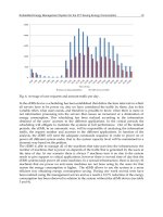
Hay (1987) considers the use of the load duration
curve to model variable thermal and electrical loads in
system sizing, along with four different scenarios de-
scribed in Figure 7.14. Each one of these scenarios deﬁ nes
an operating alternative associated to a system size.
Oven (1991) discusses the use of the load duration
curve to model variable thermal and electrical loads in
system sizing in conjunction with required thermal and
electrical load factors. Given the thermal load dura-
tion and electrical load duration curves for a particular
facility, different sizing alternatives can be deﬁ ned for
various load factors.

Eastey et al. (1984) discusses a model (CO-
GENOPT) for sizing cogeneration systems. The basic
inputs to the model are a set of thermal and electric
proﬁ les, the cost of fuels and electricity, equipment cost
and performance for a particular technology. The model
calculates the operating costs and the number of units
for different system sizes. Then it estimates the net pres-
ent value for each one of them. Based on the maximum
net present value, the “optimum” system is selected. The
model includes cost and load escalation.
Wong, Ganesh and Turner (1991) have developed
two statistical computer models to optimize cogenera-
tion system size subject to varying capacities/loads and
Figure 7-14. Each operation mode deﬁ nes a sizing alternative. Source: Hay (1987).
174 ENERGY MANAGEMENT HANDBOOK
to meet an availability requirement. One model is for
internal combustion engines and the other for unﬁ red gas
turbine cogeneration systems. Once the user deﬁ nes a re-
quired availability, the models determine the system size
or capacity that meets the required availability and maxi-
mizes the expected annual worth of its life cycle cost.
7.3 COMPUTER PROGRAMS
There are several computer programs-mainly PC
based-available for detailed evaluation of cogeneration
systems. In opposition to the rather simple methods
discussed above, CHP programs are intended for system
conﬁ guration or detailed design and analysis. For these
reasons, they require a vast amount of input data. Below,
we examine two of the most well known programs.
7.3.1 CELCAP

Lee (1988) reports that the Naval Civil Engineer-
ing Laboratory developed a cogeneration analysis com-
puter program known as Civil Engineering Laboratory
Cogeneration Program (CELCAP), “for the purpose of
evaluating the performance of cogeneration systems on
a lifecycle operating cost basis.” He states that “selec-
tion of a cogeneration energy system for a speciﬁ c ap-
plication is a complex task.” He points out that the ﬁ rst
step in the selection of cogeneration system is to make
a list of potential candidates. These candidates should
include single or multiple combinations of the various
types of engine available. The computer program does
not specify CHP systems; these must be selected by the
designer. Thus, depending on the training and previous
experience of the designer, different designers may se-
lect different systems of different sizes. After selecting a
short-list of candidates, modes of operations are deﬁ ned
for the candidates. So, if there are N candidates and
M modes of operation, then NxM alternatives must be
evaluated. Lee considers three modes of operation:
1) Prime movers operating at their full-rated capacity,
any excess electricity is sold to the utility and any
excess heat is rejected to the environment. Any
electricity shortage is made up with imports. Pro-
cess steam shortages are made-up by an auxiliary
boiler.
2) Prime movers are specified to always meet the
entire electrical load of the user. Steam or heat
demand is met by the prime mover. An auxiliary
boiler is ﬁ red to meet any excess heat deﬁ cit and

excess heat is rejected to the environment.
3) Prime movers are operated to just meet the steam
or heat load. In this mode, power deﬁ cits are made
up by purchased electricity. Similarly, any excess
power is sold back to the utility.
For load analysis, Lee considers that “demand of the
user is continuously changing. This requires that data on
the electrical and thermal demands of the user be avail-
able for at least one year.” He further states that “electri-
cal and heat demands of a user vary during the year be-
cause of the changing working and weather conditions.”
However, for evaluation purposes, he assumes that the
working conditions of the user-production related CHP
load-remain constant and “that the energy-demand pat-
tern does not change signiﬁ cantly from year to year.”
Thus, to consider working condition variations, Lee clas-
siﬁ es the days of the year as working and non-working
days. Then, he uses “average” monthly load proﬁ les and
“typical” 24-hour load proﬁ les for each class.
“Average” load proﬁ les are based on electric and
steam consumption for an average weather condition at
the site. A load proﬁ le is developed for each month, thus
monthly weather and consumption data is required. A
best ﬁ t of consumption (Btu/month or kWh/month)
versus heating and cooling degree days is thus obtained.
Then, actual hourly load proﬁ les for working and non-
working days for each month of the year are developed.
The “best representative” proﬁ le is then chosen for the
“typical working day” of the month. A similar proce-
dure is done for the non-working days.

Next an energy balance or reconciliation is per-
formed to make sure the consumption of the hourly
load proﬁ les agrees with the monthly energy usage. A
multiplying factor K is deﬁ ned to adjust load proﬁ les
that do not balance.
K
j
= E
mj
/(AE
wj
+ AE
nwj
) (7.9)
where
K
j
= multiplying factor for month j
E
mj
= average consumption (kWh) by the user for
the month j selected from the monthly elec-
tricity usage versus degree day plot
AE
wj
= typical working-day electric usage (kWh),
i.e. the area under the typical working day
electric demand proﬁ le for the month j
AE
nwj

= typical non-working day usage (kWh), i.e.
the area under the typical non-working day
electric demand proﬁ le for the month j.
Lee suggests that each hourly load in the load
proﬁ les be multiplied by the K factor to obtain the “cor-
COGENERATION AND DISTRIBUTED GENERATION 175
rect working and non-working day load proﬁ les for the
month.” The procedure is repeated for all months of the
year for both electric and steam demands. Lee states that
“the resulting load proﬁ les represent the load demand
for average weather conditions.”
Once a number of candidate CHP systems has
been selected, equipment performance data and the load
proﬁ les are fed into CELCAP to produce the required
output. The output can be obtained in a brief or detailed
form. In brief form, the output consists of a summary of
input data and a life cycle cost analysis including fuel,
operation and maintenance and purchased power costs.
The detailed printout includes all the information of the
brief printout, plus hourly performance data for 2 days
in each month of the year. It also includes the maximum
hourly CHP output and fuel consumption. The hourly
electric demand and supply are plotted, along with the
hourly steam demand and supply for each month of the
year.
Despite the simplifying assumptions introduced by
Lee to generate average monthly and typical daily load
proﬁ les, it is evident that still a large amount of data
handling and preparation is required before CELCAP
is run. By recognizing the fact that CHP loads vary

over time, he implicitly justiﬁ es the amount of effort in
representing the input data through hourly proﬁ les for
typical working and non-working days of the month.
If a change occurs in the products, process or
equipment that constitute the energy consumers within
the industrial plant, a new set of load proﬁ les must be
generated. Thus, exploring different conditions requires
sensitivity analyses or parametric studies for off-design
conditions.
A problem that becomes evident at this point
is that, to accurately represent varying loads, a large
number of load data points must be estimated for sub-
sequent use in the computer program. Conversely, the
preliminary feasibility evaluation methods discussed
previously, require very few and only “average” load
data. However, criticism of preliminary methods has
arisen for not being able to truly reﬂ ect seasonal varia-
tions in load analysis (and economic analysis) and for
lacking the ﬂ exibility to represent varying CHP system
performance at varying loads.
7.3.2 COGENMASTER
Limaye and Balakrishnan (1989) of Synergic Re-
sources Corporation have developed COGENMASTER.
It is a computer program to model the technical aspects
of alternative cogeneration systems and options, evalu-
ate economic feasibility, and prepare detailed cash ﬂ ow
statements.
COGENMASTER compares the CHP alternatives
to a base case system where electricity is purchased from
the utility and thermal energy is generated at the site.

They extend the concept of an option by referring not
only to different technologies and operating strategies
but also to different ownership structures and ﬁ nanc-
ing arrangements. The program has two main sections:
a Technology and a Financial Section. The technology
Section includes 5 modules:
• Technology Database Module
• Rates Module
• Load Module
• Sizing Module
• Operating Module
The Financial Section includes 3 modules:
• Financing Module
• Cash Flow Module
• Pricing Module
In COGENMASTER, facility electric and thermal
loads may be entered in one of three ways, depending
on the available data and the detail required for project
evaluation:
— A constant average load for every hour of the year.
— Hourly data for three typical days of the year
— Hourly data for three typical days of each month
Thermal loads may be in the form of hot water or
steam; but system outlet conditions must be speciﬁ ed
by the user. The sizing and operating modules permit
a variety of alternatives and combinations to be con-
sidered. The system may be sized for the base or peak,
summer or winter, and electric or thermal load. There is
also an option for the user to deﬁ ne the size the system
in kilowatts. Once the system size is deﬁ ned, several

operation modes may be selected. The system may be
operated in the electric following, thermal following or
constantly running modes of operation. Thus, N sizing
options and M operations modes deﬁ ne a total of NxM
cogeneration alternatives, from which the “best” alterna-
tive must be selected. The economic analysis is based on
simple payback estimates for the CHP candidates versus
a base case or do-nothing scenario. Next, depending
on the ﬁ nancing options available, different cash ﬂ ows
may be deﬁ ned and further economic analysis-based
176 ENERGY MANAGEMENT HANDBOOK
on the Net Present Value of the alternatives—may be
performed.
7.4 U.S. COGENERATION LEGISLATION: PURPA
In 1978 the U.S. Congress amended the Federal Power
Act by promulgation of the Public Utilities Regulatory
Act (PURPA). The Act recognized the energy saving
potential of industrial cogeneration and small power
plants, the need for real and signiﬁ cant incentives for
development of these facilities and the private sector
requirement to remain unregulated.
PURPA of 1978 eliminated several obstacles to
cogeneration so cogenerators can count on “fair” treat-
ment by the local electric utility with regard to intercon-
nection, back-up power supplies, and the sale of excess
power. PURPA contains the major federal initiatives
regarding cogeneration and small power production.
These initiatives are stated as rules and regulations
pertaining to PURPA Sections 210 and 201; which were
issued in ﬁ nal form in February and March of 1980,

respectively. These rules and regulations are discussed
in the following sections.
Initially, several utilities—especially those with
excess capacity-were reticent to buy cogenerated power
and have, in the past, contested PURPA. Power (1980)
magazine reported several cases in which opposition
persisted in some utilities to private cogeneration. But
after the Supreme Court ruling in favor of PURPA, more
and more utilities are ﬁ nding that PURPA can work to
their advantage. Polsky and Landry (1987) report that
some utilities are changing attitudes and are even invest-
ing in cogeneration projects.
7.4.1 PURPA 201*
Section 201 of PURPA requires the Federal Energy
Regulatory Commission (FERC) to deﬁ ne the criteria
and procedures by which small power producers (SPPs)
and cogeneration facilities can obtain qualifying status
to receive the rate beneﬁ ts and exemptions set forth in
Section 210 of PURPA. Some PURPA 201 deﬁ nitions are
stated below.
Small Power Production Facility
A “Small Power Production Facility” is a facility
that uses biomass, waste, or renewable resources, includ-
ing wind, solar and water, to produce electric power and
is not greater than 80 megawatts.
Facilities less than 30 MW are exempt from the
Public Utility Holding Co. Act and certain state law
and regulation. Plants of 30 to 80 MW which use bio-
mass, may be exempted from the above but may not
be exempted from certain sections of the Federal Power

Act.
Cogeneration Facility
A “Cogeneration Facility” is a facility which pro-
duces electric energy and forms of useful thermal energy
(such as heat or steam) used for industrial, commercial,
heating or cooling purposes, through the sequential use
of energy. A Qualifying Facility (QF) must meet certain
minimum efﬁ ciency standards as described later. Co-
generation facilities are generally classiﬁ ed as “topping”
cycle or “bottoming” cycle facilities.
7.4.2 Qualiﬁ cation of a “Cogeneration Facility” or a
“Small Power Production Facility” under PURPA
Cogeneration Facilities
To distinguish new cogeneration facilities which
will achieve meaningful energy conservation from
those which would be “token” facilities producing
trivial amounts of either useful heat or power, the FERC
rules establish operating and efﬁ ciency standards for
both topping-cycle and bottom-cycle NEW cogenera-
tion facilities. No efﬁ ciency standards are required for
EXISTING cogeneration facilities regardless of energy
source or type of facility. The following fuel utilization
effectiveness (FUE) values—based on the lower heating
value (LHV) of the fuel—are required from QFs.
• For a new topping-cycle facility:
— No less than 5% of the total annual energy
output of the facility must be useful thermal
energy.
• For any new topping-cycle facility that uses any
natural gas or oil:

— All the useful electric power and half the use-
ful thermal energy must equal at least 42.5%
of the total annual natural gas and oil energy
input; and
— If the useful thermal output of a facility is less
than 15% of the total energy output of the facil-
ity, the useful power output plus one-half the
useful thermal energy output must be no less
than 45% of the total energy input of natural
gas and oil for the calendar.
*Most of the following sections have been adapted from CFR18 (1990)
and Harkins (1980), unless quoted otherwise.
COGENERATION AND DISTRIBUTED GENERATION 177
For a new bottoming-cycle facility:
• If supplementary ﬁ ring (heating of water or steam
before entering the electricity generation cycle
from the thermal energy cycle) is done with oil
or gas, the useful power output of the bottoming
cycle must, during any calendar year, be no less
than 45% of the energy input of natural gas and
oil for supplementary ﬁ ring.
Small Power Production Facilities
To qualify as a small power production facility
under PURPA, the facility must have production capac-
ity of under 80 MW and must get more than 50% of its
total energy input from biomass, waste, or renewable
resources. Also, use of oil, coal, or natural gas by the
facility may not exceed 25% of total annual energy input
to the facility.
Ownership Rules Applying to

Cogeneration and Small Power Producers
A qualifying facility may not have more than 50%
of the equal interest in the facility held by an electric
utility.
7.4.3 PURPA 210
Section 210 of PURPA directs the Federal Energy
Regulatory Commission (FERC) to establish the rules
and regulations requiring electric utilities to purchase
electric power from and sell electric power to qualifying
cogeneration and small power production facilities and
provide for the exemption to qualifying facilities (QF)
from certain federal and state regulations.
Thus, FERC issued in 1980 a series of rules to relax
obstacles to cogeneration. Such rules implement sections
of the 1978 PURPA and include detailed instructions to
state utility commissions that all utilities must purchase
electricity from cogenerators and small power producers
at the utilities’ “avoided” cost. In a nutshell, this means
that rates paid by utilities for such electricity must re-
ﬂ ect the cost savings they realize by being able to avoid
capacity additions and fuel usage of their own.
Tuttle (1980) states that prior to PURPA 210, cogen-
eration facilities wishing to sell their power were faced
with three major obstacles:
• Utilities had no obligation to purchase power, and
contended that cogeneration facilities were too
small and unreliable. As a result, even those co-
generators able to sell power had difﬁ culty getting
an equitable price.
• Utility rates for backup power were high and often

discriminatory
• Cogenerators often were subject to the same strict
state and federal regulations as the utility.
PURPA was designed to remove these obstacles,
by requiring utilities to develop an equitable program
of integrating cogenerated power into their loads.
Avoided Costs
The costs avoided by a utility when a cogeneration
plant displaces generation capacity and/or fuel usage
are the basis to set the rates paid by utilities for co-
generated power sold back to the utility grid. In some
circumstances, the actual rates may be higher or lower
than the avoided costs, depending on the need of the
utility for additional power and on the outcomes of the
negotiations between the parties involved in the cogen-
eration development process.
All utilities are now required by PURPA to provide
data regarding present and future electricity costs on a
cent-per-kWh basis during daily, seasonal, peak and off-
peak periods for the next ﬁ ve years. This information
must also include estimates on planned utility capacity
additions and retirements, and cost of new capacity and
energy costs.
Tuttle (1980) points out that utilities may agree to
pay greater price for power if a cogeneration facility
can:
• Furnish information on demonstrated reliability
and term of commitment.
• Allow the utility to regulate the power produc-
tion for better control of its load and demand

changes.
• Schedule maintenance outages for low-demand
periods.
• Provide energy during utility-system daily and
seasonal peaks and emergencies.
• Reduce in-house on-site load usage during emer-
gencies.
• Avoid line losses the utility otherwise would have
incurred.
In conclusion, a utility is willing to pay better
“buyback” rates for cogenerated power if it is short in
capacity, if it can exercise a level of control on the CHP
plant and load, and if the cogenerator can provide and/
or demonstrate a “high” system availability.
178 ENERGY MANAGEMENT HANDBOOK
PURPA further states that the utility is not obligat-
ed to purchase electricity from a QF during periods that
would result in net increases in its operating costs. Thus,
low demand periods must be identiﬁ ed by the utility
and the cogenerator must be notiﬁ ed in advance. Dur-
ing emergencies (utility outages), the QF is not required
to provide more power than its contract requires, but a
utility has the right to discontinue power purchases if
they contribute to the outage.
7.4.4 Other Regulations
Several U.S. regulations are related to cogenera-
tion. For example, among environmental regulations,
the Clean Air Act may control emissions from a waste-
to-energy power plant. Another example is the regu-
lation of underground storage tanks by the Resource

Conservation and Recovery Act (RCRA). This applies to
all those cogenerators that store liquid fuels in under-
ground tanks. Thus, to maximize beneﬁ ts and to avoid
costly penalties, cogeneration planners and developers
should become savvy in related environmental mat-
ters.
There are many other issues that affect the de-
velopment and operation of a cogeneration project.
For further study, the reader is referred to a variety of
sources such proceedings from the various World En-
ergy Engineering Congresses organized by the Associa-
tion of Energy Engineers (Atlanta, GA). Other sources
include a general compendium of cogeneration planning
considerations given by Orlando (1990), and a manual-
developed by Spiewak (1994)—which emphasizes the
regulatory, contracting and ﬁ nancing issues of cogenera-
tion.
7.5 EVALUATING COGENERATION
OPPORTUNITIES: CASE EXAMPLES
The feasibility evaluation of cogeneration opportunities
for both, new construction and facility retroﬁ t, require
the comparison and ranking of various options using a
ﬁ gure of economic merit. The options are usually combi-
nations of different CHP technologies, operating modes
and equipment sizes.
A ﬁ rst step in the evaluation is the determination
of the costs of a base-case (or do-nothing) scenario.
For new facilities, buying thermal and electrical energy
from utility companies is traditionally considered the
base case. For retroﬁ ts, the present way to buy and/or

generate energy is the base case. For many, the base-case
scenario is the “actual plant situation” after “basic” en-
ergy conservation and management measures have been
implemented. That is, cogeneration should be evaluated
upon an “efﬁ cient” base case plant.
Next, suitable cogeneration alternatives are gener-
ated using the methods discussed in sections 7.2 and
7.3. Then, the comparison and ranking of the base case
versus the alternative cases is performed using an eco-
nomic analysis.
Henceforth, this section addresses a basic approach
for the economic analysis of cogeneration. Speciﬁ cally,
it discusses the development of the cash ﬂ ows for each
option including the base case. It also discusses some
ﬁ gures of merit such as the gross pay out period (simple
payback) and the discounted or internal rate of return.
Finally, it describes two case examples of evaluations in
industrial plants. The examples are included for illustra-
tive purposes and do not necessarily reﬂ ect the latest
available performance levels or capital costs.
7.5.1 General Considerations
A detailed treatise on engineering economy is pre-
sented in Chapter 4. Even so, since economic evaluations
play the key role in determining whether cogeneration
can be justiﬁ ed, a brief discussion of economic consid-
erations and several evaluation techniques follows.
The economic evaluations are based on examining
the incremental increase in the investment cost for the
alternative being considered relative to the alternative
to which it is being compared and determining whether

the savings in annual operating cost justify the increased
investment. The parameter used to evaluate the eco-
nomic merit may be a relatively simple parameter such
as the “gross payout period.” Or one might use more
sophisticated techniques which include the time value of
money, such as the “discounted rate of return,” on the
discretionary investment for the cogeneration systems
being evaluated.
Investment cost and operating cost are the expen-
diture categories involved in an economic evaluation.
Operating costs result from the operations of equipment,
such as (1) purchased fuel, (2) purchased power, (3) pur-
chased water, (4) operating labor, (5) chemicals, and (6)
maintenance. Investment-associated costs are of primary
importance when factoring the impact of federal and
state income taxes into the economic evaluation. These
costs (or credits) include (1) investment tax credits, (2)
depreciation, (3) local property taxes, and (4) insurance.
The economic evaluation establishes whether the op-
erating and investment cost factors result in sufﬁ cient
after-tax income to provide the company stockholders
an adequate rate of return after the debt obligations with
regard to the investment have been satisﬁ ed.
When one has many alternatives to evaluate, the
COGENERATION AND DISTRIBUTED GENERATION 179
less sophisticated techniques, such as “gross payout,”
can provide an easy method for quickly ranking al-
ternatives and eliminating alternatives that may be
particularly unattractive. However, these techniques are
applicable only if annual operating costs do not change

signiﬁ cantly with time and additional investments do
not have to be made during the study period.
The techniques that include the time value of
money permit evaluations where annual savings can
change signiﬁ cantly each year. Also, these evaluation
procedures permit additional investments at any time
during the study period. Thus these techniques truly
reﬂ ect the proﬁ tability of a cogeneration investment or
investments.
7.5.2 Cogeneration Evaluation Case Examples
The following examples illustrate evaluation proce-
dures used for cogeneration studies. Both examples are
based on 1980 investment costs for facilities located in
the U.S. Gulf Coast area.
For simplicity, the economic merit of each alterna-
tive examined is expressed as the “gross payout period”
(GPO). The GPO is equal to the incremental investment
for cogeneration divided by the resulting ﬁ rst-year an-
nual operating cost savings. The GPO can be converted
to a “discounted rate of return” (DRR) using Figure 7.15.
However, this curve is valid only for evaluations involv-
ing a single investment with ﬁ xed annual operating cost
savings with time. In most instances, the annual savings
due to cogeneration will increase as fuel costs increase
to both utilities and industries in the years ahead. These
increased future savings enhance the economics of co-
generation. For example, if we assume that a project has a
GPO of three years based on the ﬁ rst-year operating cost
savings, Figure 7.15 shows a DRR of 18.7%. However, if
the savings due to cogeneration increase 10% annually

for the ﬁ rst three operating years of the project and are
constant thereafter, the DRR increases to 21.6%; if the sav-
ings increase 10% annually for the ﬁ rst six years, the DRR
would be 24.5%; and if the 10% increase was experienced
for the ﬁ rst 10 years, the DRR would be 26.6%.
Example 6: The energy requirements for a large in-
dustrial plant are given in Table 7.3. The alternatives
considered include:
Base case. Three half-size coal-ﬁ red process boilers are
installed to supply steam to the plant’s 250-psig steam
header. All 80-psig steam and steam to the 20-psig deaer-
ating heater is pressure-reduced from the 250-psig steam
header. The powerhouse auxiliary power requirements
are 3.2 MW. Thus the utility tie must provide 33.2 MW
to satisfy the average plant electric power needs.
Case 1. This alternative is based on installation of a
noncondensing steam turbine generator. The unit initial
Table 7.3 Plant Energy Supply System Considerations: Example 6
———————————————————————————————————————————————————
Process steam demands
Net heat to process at 250 psig. 410°F—317 million Btu/hr avg.
Net heat to process at 80 psig, 330°F—208 million Btu/hr avg. (peak requirements are 10% greater than
average values)
Process condensate returns: 50% of steam delivered at 280°F
Makeup water at 80°F
Plant fuel is 3.5% sulfur coal
Coal and limestone for SO
2
scrubbing are available at a total cost of $2/million Btu ﬁ red
Process area power requirement is 30 MW avg.

Purchased power cost is 3.5 cents/kWh
———————————————————————————————————————————————————
Fig. 7.15 Discounted rate of return versus gross payout
period. Basis: (1) depreciation period, 28 years; (2) sum-
of-the-years’-digits depreciation; (3) economic life, 28
years; (4) constant annual savings with time; (5) local
property taxes and insurance, 4% of investment cost;
(6) state and federal income taxes, 53%; (7) investment
tax credit, 10% of investment cost.
180 ENERGY MANAGEMENT HANDBOOK
steam conditions are 1450 psig, 950°F with automatic
extraction at 250 psig and 80 psig exhaust pressure.
The boiler plant has three half-size units providing the
same reliability of steam supply as the Base Case. The
feedwater heating system has closed feedwater heat-
ers at 250 psig and 80 psig with a 20 psig deaerating
heater. The 20-psig steam is supplied by noncondensing
mechanical drive turbines used as powerhouse auxiliary
drives. These units are supplied throttle steam from the
250-psig steam header. For this alternative, the utility tie
normally provides 4.95 MW. The simpliﬁ ed schematic
and energy balance is given in Figure 7.16.
The results of this cogeneration example are tabu-
lated in Table 7.4. Included are the annual energy re-
quirements, the 1980 investment costs for each case, and
the annual operating cost summary. The investment cost
data presented are for fully operational plants, includ-
ing ofﬁ ces, stockrooms, machine shop facilities, locker
rooms, as well as ﬁ re protection and plant security. The
cost of land is not included.

The incremental investment cost for Case 1 given
in Table 7.4 is $17.2 million. Thus the incremental cost is
$609/kW for the 28.25-MW cogeneration system. This il-
lustrates the favorable per unit cost for cogeneration sys-
tems compared to coal-ﬁ red facilities designed to provide
kilowatts only, which cost in excess of $1000/kW.
The impact of fuel and purchased power costs
other than Table 7.3 values on the GPO for this example
is shown in Figure 7.17. Equivalent DRR values based
on ﬁ rst-year annual operating cost savings can be esti-
mated using Figure 7.15.
Sensitivity analyses often evaluate the impact
of uncertainties in the installed cost estimates on the
proﬁ tability of a project. If the incremental investment
cost for cogeneration is 10% greater than the Table 7.4
estimate, the GPO would increase from 3.2 to 3.5 years.
Thus the DRR would decrease from 17.5% to about 16%,
as shown in Figure 7.15.
Table 7.4 Energy and Economic Summary: Example 6
———————————————————————————————————————————————————
Alternative Base Case Case 1
———————————————————————————————————————————————————
Energy summary
Boiler fuel (10
6
Btu/hr HHV) 599 714
Purchased power (MW) 33.20 4.95
Estimated total installed cost (10
6
$) 57.6 74.8

Annual operating costs (10
6
$)
Fuel and limestone at $2/10
6
Btu 10.1 12.0
Purchased power at 3.5 cents/kWh 9.8 1.5
Operating labor 0.8 1.1
Maintenance 1.4 1.9
Makeup water 0.3 0.5
Total 22.4 17.0
Annual savings (10
6
$) Base 5.4
Gross payout period (yrs) Base 3.2
———————————————————————————————————————————————————
Basis: (1) boiler efﬁ ciency is 87%; (2) operation equivalent to 8400 hr/yr at Table 7-3 conditions; (3) maintenance
is 2.5% of the estimated total installed cost; (4) makeup water cost for case 1 is 80 cents/1000 gal greater than Base
Case water costs; (5) stack gas scrubbing based on limestone system.
———————————————————————————————————————————————————
Fig. 7.16 Simplified schematic and energy-balance
diagram: Example 6, Case 1. All numbers are ﬂ ows in
10
3
lb/hr; Plant requirements given in Table 7.8, gross
generation, 30.23 MW; powerhouse auxiliaries, 5.18
MW; net generation, 25.05 MW.
COGENERATION AND DISTRIBUTED GENERATION 181
Example 7: The energy requirements for a chemical
plant are presented in Table 7.5. The alternatives con-

sidered include:
Base case. Three half-size oil-ﬁ red packaged process boil-
ers are installed to supply process steam at 150 psig. Each
unit is fuel-oil-ﬁ red and includes a particulate removal
system. The plant has a 60-day fuel-oil-storage capacity.
A utility tie provides 30.33 MW average to supply process
and boiler plant auxiliary power requirements.
Case 1. (Refer to Figure 7.18). This alternative examines
the merit of adding a noncondensing steam turbine
generator with 850 psig, 825°F initial steam condi-
tions, 150-psig exhaust pressure. Steam is supplied by
three half-size packaged boilers. The feedwater heating
system is comprised of a 150-psig closed heater and a
20-psig deaerating heater. The steam for the deaerat-
ing heater is the exhaust of a mechanical drive turbine
(MDT). The MDT is supplied 150-psig steam and drives
Table 7.5 Plant Energy Supply System Considerations:
Example 7
—————————————————————————
Process steam demands
Net heat to process at 150 psig sat—158.5 million
Btu/hr avg. (peak steam requirements are 10%
greater than average values)
Process condensate returns: 45% of the steam delivered
at 300°F
Makeup water at 80°F
Plant fuel is fuel oil
Fuel cost is $5/million Btu
Process areas require 30 MW
Purchased power cost is 5 cents/kWh

—————————————————————————
some of the plant boiler feed pumps. The net generation
of this cogeneration system is 6.32 MW when operating
at the average 150-psig process heat demand. A utility
tie provides the balance of the power required.
Case 2. (Refer to Figure 7.19). This alternative is a com-
bined cycle using the 25,000-kW gas turbine generator
whose performance is given in Table 7.7. An unﬁ red
HRSG system provides steam at both 850 psig, 825°F
and 150 psig sat. Plant steam requirements in excess of
that available from the two-pressure level unﬁ red HRSG
system are generated in an oil ﬁ red packaged boiler.
The steam supplied to the noncondensing turbine is
expanded to the 150-psig steam header. The net genera-
tion from the overall system is 26.54 MW. A utility tie
provides power requirements in excess of that supplied
by the cogeneration system. The plant-installed cost es-
timates for Case 2 include two half-size package boilers.
Thus full steam output can be realized with any steam
generator out of service for maintenance.
The energy summary, annual operating costs, and
economic results are presented in Table 7.6. The results
show that the combined cycle provides a GPO of 2.5
years based on the study fuel and purchased power
costs. The incremental cost for Case 2 relative to the
Base Case is $395/kW compared to $655/kW for Case
1 relative to the Base Case. This favorable incremental
investment cost combined with a FCP of 5510 Btu/kWh
contribute to the low CPO.
The inﬂ uence of fuel and power costs other than

those given in Table 7.5 on the GPO for cases 1 and 2 is
Fig. 7.17
Effect of dif-
ferent fuel
and power
costs on
cogeneration
proﬁ tability:
Example 1.
Basis: Condi-
tions given
in Tables 7.3
and 7.4.
Fig. 7.18 Simplified schematic and energy-balance
diagram: Example 7, Case 1. All numbers are ﬂ ows
in 1000 lb/hr; gross generation, 6.82 MW; powerhouse
auxiliaries, 0.50 MW; net generation; 6.32 MW.
182 ENERGY MANAGEMENT HANDBOOK
shown in Figure 7.20. These GPO values can be trans-
lated to DRRs using Figure 7.15.
Example 8. A gas-turbine and HRSG cogeneration sys-
tem is being considered for a brewery to supply base-
load electrical power and part of the steam needed for
process. An overview of the proposed system is shown
in Figure 7.21. This example shows the use of computer
tools in cogeneration design and evaluation.
Base Case.: Currently, the plant purchases about
3,500,000 kWh per month at $0.06 per kWh. The brew-
ery uses an average of 24,000 lb/hr of 30 psig saturated
steam. Three 300-BHP gas ﬁ red boilers produce steam

Table 7.6 Energy and Economic Summary: Example 7
———————————————————————————————————————————————————
Alternative Base Case Case 1 Case 2
———————————————————————————————————————————————————
Energy summary
Fuel (10
6
Btu/hr HHV)
Boiler 183 209 34
Gas turbine — 297
Total 183 209 331
Purchased power (MW) 30.33 23.77 3.48
Estimated total installed cost (10
6
$) 8.3 12.6 18.9
Annual operating cost (10
6
$)
Fuel at $5/M Btu HHV 7.7 8.8 13.9
Purchased power at 5 cents/kWh 12.7 10.0 1.5
Operating labor 0.6 0.9 0.9
Maintenance 0.2 0.3 0.5
Makeup water 0.1 0.2 0.2
Total 21.3 20.2 17.0
Annual savings (10
6
$) Base 1.1 4.3
Gross payout period (yr) Base 3.9 2.5
———————————————————————————————————————————————————
Basis: (1) gas turbine performance per Table 7-7; (2) boiler efﬁ ciency, 87%; (3) operation equivalent to 8400 hr/yr

at Table 7-5 conditions; (4) maintenance, 2.5% of the estimated total installed costs; (5) incremental makeup water
cost for cases 1 and 2 relative to the Base Case. $1 /1000 gal.
Fig. 7.19 Simpliﬁ ed schematic and
energy-balance diagram: Example
7, Case 2. All numbers are ﬂ ows in
1000 lb/hr; gross generation, 26.77
MW, powerhouse auxiliaries, 0.23
MW: net generation, 26.54 MW.
at 35 psig, to allow for pressure losses. The minimum
steam demand is 10,000 lb/hr. The plant operates con-
tinuously during ten months or 7,000 hr/year. The base
or minimum electrical load during production is 3,200
kW. The rest of the time (winter) the brewery is down
for maintenance. The gas costs $3.50/MMBtu.
Case 1: Consider the gas turbine whose ratings are given
on Figure 7.11. We will evaluate this turbine in conjunc-
tion with an unﬁ red water-tube HRSG to supply part of
the brewery’s heat and power loads. First, we obtain the
ratings and performance data for the selected turbine,
which has been sized to meet the electrical base load (3.5
MW). An air washer/evaporative cooler will be installed
COGENERATION AND DISTRIBUTED GENERATION 183
at the turbine inlet to improve (reduce) the overall heat
rate by precooling the inlet air to an average 70°F (80°F
or less), during the summer production season Addi-
tional operating data are given below.
Operating Data
Inlet air pressure losses (ﬁ lter and air
pre-cooler): 5” H
2

O
Exhaust Losses (ducting, by-pass valve,
HRSG and Stack): 12” H
2
O
Location Elevation above sea level: 850 ft
Thus, on a preliminary basis, we assume the tur-
bine will constantly run at full capacity, minus the effect
of elevation, the inlet air pressure drop and exhaust
losses. Since the plant will be located at 850 ft above sea
level, from Figure 7.11, the elevation correction factor
is 0.90. Hence, the corrected continuous power rating
(before deducting pressure losses) when ﬁ ring natural
gas and using 70°F inlet air is:
Table 7.7 Steam Generation and Fuel Chargeable to Power: 25,000-kW ISO Gas Turbine and HRSG (Distillate
Oil Fuel)
a
———————————————————————————————————————————————————
Type HRSG Unﬁ red Supplementary Fired Fully Fired
———————————————————————————————————————————————————
Gas Turbine
Fuel (10
6
Btu/hr HHV) 297
Output (MW) 21.8 21.6 21.4
Airﬂ ow (10
3
lb/hr) 915
Exhaust temperature (°F) 920 922 925
HRSG fuel (10

6
Btu/hr HHV) NA 190 769

Steam FCP Steam FCP Steam FCP
(10
3
lb/hr) (Btu/kWh HHV) (10
3
lb/hr) (Btu/kWh HHV) (10
3
lb/hr) (Btu/kWh HHV)
Steam conditions
250 psig sat. 133 6560 317 5620 851 4010
400 psig, 650°F 110 7020 279 5630 751
600 psig, 750°F 101 7340 268 5660 722
850 psig, 825°F 93 7650 261 5700 703
1250 psig, 900°F — — 254 5750 687
1450 psig, 950°F — — 250 5750 675
———————————————————————————————————————————————————
a
Basis: (1) gas turbine performance given for 80°F ambient temperature, sea-level site; (2) HRSG performance based on 3%
blowdown, 1-1/2% radiation and unaccounted losses, 228°F feedwater; (3) no HRSG bypass stack loss; (4) gas turbine exhaust
pressure loss is 10 in. H
2
O with unﬁ red, 14 in. H
2
O with supplementary ﬁ red, and 20 in. H
2
O with fully ﬁ red HRSG; (5) fully
ﬁ red HRSG based on 10% excess air following the ﬁ ring system and 300°F stack. (6) fuel chargeable to gas turbine power

assumes total fuel credited with equivalent 88% boiler fuel required to generate steam; (7) steam conditions are at utilization
equipment; a 5% AP and 5°F AT have been assumed from the outlet of the HRSG.
®
†
®
Fig. 7.20 Effect of different fuel and power cost on co-
generation proﬁ tability: Example 2. Basis: Conditions
given in Tables 7.4 and 7.5.
184 ENERGY MANAGEMENT HANDBOOK
= (Generator Output @ 70°F)
(Elevation correction @ 850 ft)
= 4,200 kWe × 0.9
= 3,780 kWe
Next, by using the Inlet and Exhaust Power Loss
graphs in Figure 7.11, we get the exhaust and inlet
losses (@ 3780 kW output): 17 and 7 kW/inch H
2
O,
respectively. So, the total power losses due to inlet and
exhaust losses are:
= (17 in)(5 kW/in) + (12 in)(8 kW/in)
= 181 kW
Consequently, the net turbine output after elevation and
pressure losses is
= 3,780 - 181
= 3,599 kWe
Next, from Figure 7.11 we get the following performance
data for 70°F inlet air:
Heat rate : 12,250 Btu/kWh (LHV)
Exhaust Temperature : 935°F

Exhaust Flow : 160,000 lb/hr
These ﬁ gures have been used as input data for
HGPRO—a prototype HRSG software program devel-
oped by V. Ganesh, W.C. Turner and J.B. Wong in 1992
at Oklahoma State University. The program results are
shown in Fig. 7.22.
The total installed cost of the complete cogenera-
tion plant including gas turbine, inlet air precooling,
HRSG, auxiliary equipment and computer based con-
trols is $4,500,000. Fuel for cogeneration is available on
a long term contract basis (>5 years) at $2.50/MMBtu.
The brewery has a 12% cost of capital. Using a 10-year
after tax cash ﬂ ow analysis with current depreciation
and tax rates, should the brewery invest in this cogen-
eration option? For this evaluation, assume: (1) A 1%
inﬂ ation for power and non-cogen natural gas; (2) an
operation and maintenance (O&M) cost of $0.003/kWh
for the ﬁ rst year after the project is installed. Then, the
O&M cost should escalate at 3% per year; (3) the plant
salvage value is neglected.
Economic Analysis
Next, we present system operation assumptions
required to conduct a preliminary economic analysis.
1) The cogeneration system will operate during all
the production season (7,000 hrs/year).
2) The cogeneration system will supply an average
of 3.5 MW of electrical power and 24,000 lb of 35
psig steam per hour. The HRSG will be provided
with an inlet gas damper control system to modu-
late and by-pass hot gas ﬂ ow. This is to allow for

variable steam production or steam load-following
operation.
3) The balance of power will be obtained from the
existing utility at the current cost ($0.06/kWh)
4) The existing boilers will remain as back-up units.
Any steam deﬁ cit (considered to be negligible) will
be produced by the existing boiler plant.
5) The cogeneration fuel (natural gas) will be metered
with a dedicated station and will be available at
Figure 7.21 Gas turbine/HRSG cogeneration application.
COGENERATION AND DISTRIBUTED GENERATION 185
Figure 7.22 Results from HGPRO 1.0, a
prototype HRSG software.
$2.50/MMBtu during the ﬁ rst ﬁ ve years and at
$2.75/MMBtu during the next five-year period.
Non cogeneration fuel will be available at the cur-
rent price of $3.50/MMBtu.
The discounted cash ﬂ ow analysis was carried out
using an electronic spreadsheet (Table 7.8). The results
of the spreadsheet show a positive net present value.
Therefore, when using the data and assumptions given
in this case, the cogeneration project appears to be cost
effective. The brewery should consider this project for
funding and implementation.
Note: These numbers ignore breakdowns and pos-
sible ratchet clause effects.
7.6 CLOSURE
Cogeneration has been used for almost a century to
supply both process heat and power in many large
industrial plants in the United States. This technology

would have been applied to a greater extent if we did
not experience a period of plentiful low-cost fuel and
reliable low-cost electric power in the 25 years follow-
ing the end of World War 11. Thus economic rather than
technical considerations have limited the application of
this energy-saving technology.
The continued increase in the cost of energy is
the primary factor contributing to the renewed inter-
est in cogeneration and its potential benefits. This
chapter discusses the various prime movers that
merit consideration when evaluating this technology.
Furthermore, approximate performance levels and
techniques for developing effective cogeneration sys-
tems are presented.
The cost of all forms of energy is rising sharply.
Cogeneration should remain an important factor in ef-
fectively using our energy supplies and economically
providing goods and services in those base-load ap-
plications requiring large quantities of process heat and
power.
7.6 REFERENCES
1. Butler, C.H., (1984), Cogeneration: Engineering, Design
Financing, and Regulatory Compliance, McGraw-Hill,
Inc., New York, N.Y.
2. Caton, J.A., et al., (1987), Cogeneration Systems, Texas
A&M University, College Station, TX.
3. CFR-18 (1990): Code of Federal Regulations, Part 292
Regulations Under Sections 201 and 210 of the Public
186 ENERGY MANAGEMENT HANDBOOK
COGENERATION AND DISTRIBUTED GENERATION 187

Utility Regulatory Policies Act of 1978 With Regard
to Small Power Production and Cogeneration, (4-1-90
Edition).
4. Estey P.N., et al., (1984). “A Model for Sizing Cogen-
eration Systems,” Proceedings of the 19th Intersociety
Energy Conversion Engineering Conference” Vol. 2 of
4, August, 1984, San Francisco, CA.
5. Ganapathy, V. (1991). Waste Heat Boiler Deskbook, The
Fairmont Press, Inc., Lilburn, CA.
6. Harkins H.L., (1981), “PURPA New Horizons for
Electric Utilities and Industry,” IEEE Transactions, Vol.
PAS-100, pp 27842789.
7. Hay, N., (1988), Guide to Natural Gas Cogeneration, The
Fairmont Press, Lilburn, GA.
8. Kehlhofer, R., (1991). Combined-Cycle Gas & Steam
Turbine Power Plants, The Fairmont Press, Inc. Lilburn,
Ga.
9. Kostrzewa, L.J. & Davidson, K.G., (1988). “Packaged
Cogeneration,” ASHRAE Journal, February 1988.
10. Kovacik, J.M., (1982), “Cogeneration,” in Energy Man-
agement Handbook, ed. by W.C. Turner, Wiley, New York,
N.Y.
11. Kovacik, J.M., (1985), “Industrial Cogeneration: System
Application Consideration,” Planning Cogeneration Sys-
tems, The Fairmont Press, Lilburn, Ga.
12. Lee, R.T.Y., (1988), “Cogeneration System Selection
Using the Navy’s CELCAP Code,” Energy Engineering,
Vol. 85, No. 5, 1988.
13. Limaye, D.R. and Balakrishnan, S., (1989), “Technical
and Economic Assessment of Packaged Cogeneration

Systems Using Cogenmaster,” The Cogeneration Journal,
Vol. 5, No. 1, Winter 1989-90.
14. Limaye, D.R., (1985), Planning Cogeneration Systems, The
Fairmont Press, Atlanta, CA.
15. Limaye, D.R., (1987), Industrial Cogeneration Applica-
tions, The Fairmont Press, Atlanta, CA.
16. Mackay, R. (1983). “Gas Turbine Cogeneration: Design,
Evaluation and Installation.” The Garret Corporation,
Los Angeles, CA, The Association Of Energy Engi-
neers, Los Angeles CA, February, 1983.
17. Makansi, J., (1991). “Independent Power/Cogenera-
tion, Success Breeds New Obligation-Delivering on Per-
formance,” Power, October 1991.
18. Mulloney, et. al., (1988). “Packaged Cogeneration In-
stallation Cost Experience,” Proceedings of The 11th
World Energy Engineering Congress, October 18-21,
1988.
19. Orlando, J.A., (1991). Cogeneration Planners Handbook,
The Fairmont Press, Atlanta, GA.
20. Oven, M., (1991), “Factors Affecting the Financial Vi-
ability Applications of Cogeneration,” XII Seminario
Nacional Sobre El Uso Racional de La Energia,” Mexico
City, November, 1991.
21. Polimeros, G., (1981), Energy Cogeneration Handbook,
Industrial
Press Inc., New, York.
22. Power (1980), “FERC Relaxes Obstacles to Cogenera-
tion,” Power, September 1980, pp 9-10.
23. SFA Paciﬁ c Inc. (1990). “Independent Power/Cogenera-
tion, Trends and Technology Update,” Power, October

1990.
24. Somasundaram, S., et al., (1988), A Simpliﬁ ed Self-Help
Approach To Sizing of Small-Scale Cogeneration Systems,
Texas A&M University, College Station, TX
25. Spiewak, S.A. and Weiss L., (1994) Cogeneration & Small
Power Production Manual, 4th Edition, The Fairmont
Press, Inc. Lilburn, CA.
26. Turner, W.C. (1982). Energy Management Handbook, John
Wiley & Sons, New York, N.Y.
27. Tuttle, D.J., (1980), PURPA 210: New Life for Cogenera-
tors,” Power, July, 1980.
28. Williams, D. and Good, L., (1994) Guide to the Energy
Policy Act of 1992, The Fairmont Press, Inc. Lilburn,
GA.
29. Wong, J.B., Ganesh, V. and Turner, W.C. (1991), “Sizing
Cogeneration Systems Under Variable Loads,” 14th
World Energy Engineering Congress, Atlanta, GA.
30. Wong, J.B. and Turner W.C. (1993), “Linear Optimiza-
tion of Combined Heat and Power Systems,” Indus-
trial Energy Technology Conference, Houston, March,
1993.
APPRECIATION
Many thanks to Mr. Lew Gelfand for using and
testing over the years the contents of this chapter in
the evaluation and development of actual cogeneration
opportunities, and to Mr. Scott Blaylock for the informa-
tion provided on fuel cells and microturbines. Messrs.
Gelfand and Blaylock are with DukeEnergy/DukeSolu-
tions.
188 ENERGY MANAGEMENT HANDBOOK

Appendix A
Statistical Modeling of Electric Demand and
Peak–Shaving Generator Economic Optimization
Jorge B. Wong, Ph.D., PE, CEM
ABSTRACT
This paper shows the development a basic electric
demand statistical model to obtain the optimal kW–size
and the most cost–effective operating time for an elec-
trical peak shaving generator set. This model consid-
ers the most general (and simpliﬁ ed) case of a facility
with an even monthly demand charge and a uniformly
distributed random demand, which corresponds to a
linear load–duration curve. A numerical example and
computer spreadsheet output illustrate the model.
INTRODUCTION
Throughout the world, electrical utilities include
a hefty charge in a facility’s bill for the peak electrical
demand incurred during the billing period, usually a
month. Such a charge is part of the utility’s cost recovery
or amortization of newly installed capacity and for op-
erating less efﬁ cient power plant capacity during higher
load periods.
Demand charge is a good portion of a facility’s
electrical bill. Typically a demand charge can be as
much as 50% of the bill, or more. Thus, to reduce the
demand cost, many industrial and commercial facilities
try to “manage their loads.” One example is by moving
some of the electricity–intense operations to “off–peak”
hours”—when a facility’s electrical load is much smaller
and the rates ($/kW) are lower. But, when moving elec-

trical loads to “off–peak” hours is not practical or signiﬁ -
cant, a facility will likely consider a set of engine–driven
or fuel cell generators to run in parallel with the utility
grid to supply part or all the electrical load demand
during “on–peak” hours. We call these Peak Shaving
Generators or PSGs.
While the electric load measurement is instanta-
neous, the billing demand is typically a 15–to–30– min-
ute average of the instantaneous electrical power
demand (kW). To obtain the monthly demand charge,
utilities multiply the billing demand by a demand rate.
Some utilities charge a ﬂ at rate ($/kW–peak per month)
for all months of the year. Other utilities have seasonal
charges (i.e. different rates for different seasons of the
year). Still, others use ratchet clauses to account for the
highest “on–peak” season demand of the year.
Thus, the model presented in this paper focuses on
the development of a method to obtain the optimal PSG
size (g*kW) and PSG operation time (hours per year)
for a given facility. This model is for the case of a facil-
ity with a constant billing demand rate ($/kW/month)
throughout the year. The analysis is based on a linear
load–duration curve and uses a simpliﬁ ed life–cycle–
cost approach. An example illustrates the underlying
approach and optimization method. In addition, the
paper shows an EXCEL spreadsheet to implement the
optimization model. We call this model PSG–1.
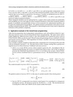
ELECTRIC DEMAND STATISTICAL MODEL
This section develops the statistical–and–math
model for the economical sizing of an electrical peak–

shaving generator set (PSG) for a given facility. The fun-
damental question is: What is the most economical genera-
tor–set size—g* in kW—for a given site demand proﬁ le?
Figure 1 shows a sample record for a facility’s electrical
demand, which is uniformly distributed between 2000
and 5300 kW. Next, Figure 2 shows the corresponding
statistical distributions.
The statistical model of electrical demand is ex-
pressed graphically in Figure 2, in terms of two func-
tions:
• The load–duration curve D(t), is the demand as a
function of cumulative time t (i.e. the accumulated
annual duration t in hrs/year of a given D(t) load
in kW), and
• The load frequency distribution f(D) (rectangular
shaded area in Figures 1 and 2) is the “uniform”
probability density function.
MODEL ASSUMPTIONS
This statistical model is based upon the following
assumptions:
1. The electrical demand is represented by a linear
load–duration curve, as shown in Figure 2. Thus,
for a typical year, the facility has a demand D
that varies between an upper value D
u
(annual
maximum) and a lower value D
1
(annual mini-
mum). This implies the electrical load is uniformly

distributed between the maximum and minimum
demands. The facility operates T hours per year.
COGENERATION AND DISTRIBUTED GENERATION 189
2. There is an even energy or consumption rate Ce
($/kWh) throughout the year.
3. There is an even demand rate Cd ($/kW/month)
for every month of the year.
4. There is a same demand peak D
u
for every month.
Demand ratchet clauses are not applicable in this
case.
5. The equipment’s annual ownership or amortiza-
tion unit installed cost ($/kW/year) is constant for
all sizes of PSGs. The unit ownership or rental cost
($/kW/year) is considered independent of unit
size. Ownership, rental or lease annualized costs
are denoted by A
c
.
6. A PSG set is installed to reduce the peak demand
by a maximum of g kW, operating t
g
hours per
year.
BASE CASE ELECTRICITY ANNUAL
COST—WITHOUT PEAK–SHAVING
Consider a facility with the load–duration charac-
teristic shown in Figures 1 and 2. For a unit consump-
tion cost Ce, the annual energy or consumption cost (with-

out PSG) for the facility is
AEC = T• D
1
• Ce + 1/2 T (D
u
– D
1
) Ce
Which is equivalent to
Figure 1. Sample record for a uniformly distributed random demand.
Figure 2. Load—Duration Curve for uniformly distributed demand.
190 ENERGY MANAGEMENT HANDBOOK
AEC = T/2 • Ce (D
u
+ D
1
) [1]
Next, considering a peak demand D
u
occurs every
month, the annual demand cost is deﬁ ned by
ADC = 12 D
u
• Cd [2]
Thus, the total annual cost for the facility is
TAC = AEC + ADC [3a]
Substituting [1] and [2] in equation [3], we have the base
case total annual cost:
TAC
1

= T/2 (D
u
+ D
1
) Ce + 12 D
u
• Cd [3b]
ELECTRICITY ANNUAL COST WITH
PEAK–SHAVING
If a peak shaving generator of size g is installed in
the facility to run in parallel with the utility grid dur-
ing peak–load hours, so the maximum load seen by the
utility is (D
u
– g), then the electric bill cost is
EBC = T/2 (D
u
– g + D
1
) Ce + 12 (D
u
– g) • Cd
In addition, the facility incurs an ownership (amor-
tization) unit cost Ac ($/kW/yr) and operation and
maintenance unit cost O&M ($/kWh). Hence, the total
annual cost with demand peak shaving is
TAC
2
= [T• D
1

+ (T+ t
g
)/2 (D
u
– g – D
1
)]Ce +
12 (D
u
– g) Cd + (Ac + 1/2 O&M • t
g
)g [4]
ANNUAL WORTH OF THE PEAK-
SHAVING GENERATOR
The annual worth or net savings AW ($/yr) of the
PSG set are obtained by subtracting equation [4] from
equation [3]. That is AW = TAC
1
– TAC
2
. So,
AW = 1/2 t
g
• g • Ce + 12 • g• Cd –
(Ac + 1/2 • O&M • t
g
)g [5]
From Figure 2 we obtain g: t
g
= (D

u
– D
1
): T
So, the expected PSG operating time is
t
g
= g • T/(D
u
– D
1
) [6]
Substituting the value of t
g
in equation [5], we have:
AW = g
2
• T/[2(D
u
– D
1
)] Ce + 12 • g • Cd –
{Ac + O&M • g • T/[2(D
u
– D
1
)]} g [7]
OPTIMUM CONDITIONS
We next determine the necessary and sufficient
conditions for an optimal PSG size g* and the corre-

sponding maximum AW to exist.
Necessary Condition
By taking the derivative of AW, Equation [7], with
respect to g and equating it to zero we obtain the nec-
essary condition for the maximum annual worth or net
saving per year. That is:
AW’ = g
• T • Ce/(D
u
– D
1
) + 12 Cd – Ac –
g • T • O&M/(D
u
– D
1
) = 0 [8]
Sufﬁ cient Condition. If the second derivative of
AW with respect to g is negative, i.e. AW”<0, then AW
(g) is a strictly convex function of g with a global maxi-
mum point. So, by taking the second derivative of AW
with respect to g and evaluating AW” as an inequality
(<0) we have:
AW” = T
• Ce/(D
u
– D
1
) – T • O&M/(D
u

– D
1
) < 0
Multiplying this equation by (D
u
– D
1
)/T we have the
sufﬁ cient condition for a maximum AW is
Ce – O&M < 0
or
Ce < O&M
Therefore, for a global maximum AW to exist, the
energy rate Ce must be less than the per unit O&M cost
(including fuel) to operate the peak shaving generator
($/kWh). Since this is the case for most utility rates Ce
and commercial PSGs O&M, we can say there is maxi-
mum AW and an optimal g* for the typical electrical
demand case.
OPTIMUM PEAK SHAVING GENERATOR SIZE
From equation [6] we can solve for g and ﬁ nd the
optimal PSG size, g* (in kW):
g* = (12 Cd – Ac) (D
u
– D
1
)/[T (O&M – Ce)] [9]
COGENERATION AND DISTRIBUTED GENERATION 191
FOR FURTHER RESEARCH
Further research is underway to develop enhanced

models which consider:
• Demand profile flexibility. Other load–duration
shapes with different underlying frequency dis-
tributions (e.g. triangular, normal and auto–cor-
related loads).
• Economies of Scale. The fact that larger units have
better fuel–to–electricity efﬁ ciencies (lower heat
rates) and lower per unit installed cost ($/kW).
__________________________________________________
EXAMPLE. A manufacturing plant operates 7500 hours
per year and has a fairly constant electrical (billing) peak
demand every month (See Figure 1). The actual load,
however, varies widely between a minimum of 2000 kW
and a maximum of 5300 kW (See Figure 2). The demand
charge is $10/kW/month and the energy charge is
$0.05/kWh. The installed cost of a diesel generator set,
the auxiliary electrical switch gear and peak–shaving
controls is about $300 per kW. Alternatively, the plant
can lease a PSG for $50/kW/yr. The operation and
maintenance cost (including diesel fuel) is $0.10/kWh.
Assuming the plant leases the PSG, estimate (1) the op-
timal PSG size, (2) the annual savings and (3) the PSG
annual operation time.
1) The optimal generator size is calculated using equa-
tion [9]
(12. $10 – $50/kWh) (5300 – 2000 kW)
g* = —————————————————
7500 h/yr ($0.10/kWh –$0.05/kWh)
= 616 kW
2) Using a commercially available PSG of size g* = 600

kW, the potential annual savings are estimated using
equation [7]
AW = g
2
• T • Ce/[2(D
u
– D
1
)] + 12 • g • Cd
– {Ac + O&M • g • T/[2(D
u
– D
1
)]} g
= 600
2
× 7500 x 0.05/(2(5300 – 2000)) + 12 × 600 × 10
– ($50 + 0.10 × 600 × 7500/(2 (5300 – 2000))) 600
= $20,455 + $72,000 – $70,909
= $21,546/year
3) The expected annual operating time for the PSG is
estimated using Equation [6]
Figure 3. PSG-1 Spreadsheet and Chart
192 ENERGY MANAGEMENT HANDBOOK
t
g
= g • T/(D
u
– D
1

)
= 600 × 7500/(5300–2000)
= 1,364 hours/year
The Excel spreadsheet and chart used to solve this case
example is shown in Figure 3.
CONCLUDING REMARKS
The reader should note that the underlying statis-
tical and optimization model is quite “responsive and
robust.” That is, the underlying methodology can be
used in, or adapted to, a variety of demand proﬁ les and
rates, while the results remain relatively valid. A forth-
coming paper by this author will show how to adapt
the linear load– duration models of Figures 1 and 2 to
more complex demand proﬁ les. Thus, for example, one
typical case is when the electrical load is represented by
a Gauss or normal distribution. Also, we will show how
to apply equation [9] to more involved industrial cases
with multiple billing seasons and demand rates.
Appendix References
Beightler, C.S., Phillips, D.T., and Wilde, D.J., Founda-
tions of Optimization, Prentice–Hall, Englewood
Cliffs, 1979.
Turner, W.C., Energy Management Handbook, 4th Edition,
the Fairmont Press, Lilburn, GA, 2001.
Hahn & Shapiro, Statistical Models in Engineering, John
Wiley 1967, Wiley Classics Library, reprinted in
1994.
Witte, L.C., Schmidt, P.S., and Brown, D.R, Industrial
Energy Management and Utilization, Hemisphere
Publishing Co. and Springer–Verlag, Berlin, 1988.

Appendix Nomenclature
Ac Equipment ownership, lease or rental cost ($/kW/
year)
ADC Annual Demand Cost ($/year)
AEC Annual Energy Cost ($/year)
AW Annual Worth ($/year)
Cd Electric demand unit cost ($/kW/month)
Ce Electric energy unit cost ($/kWh)
D Electric demand or load (kW)
D
1
Lower bound of a facility’s electric demand or
minimum load (kW)
D
u
Upper bound of a facility’s electric demand or
maximum load (kW)
EBC Electric bill cost for a facility with PSG, ($/
year)
f(D) Frequency of occurrence of a demand, (unit less)
O&M Operation and Maintenance cost, including fuel
cost ($/kWh)
g Peak shaving generator size or rated output capac-
ity (kW)
g* Optimal peak shaving generator size or output
capacity (kW)
t Time, duration of a given load, (hours/year)
t
g
Expected time of operation for a PSG, hours/

year
T Facility operation time using power(hours/year)
TAC Total annual electric cost
TAC
1
Total annual cost, base case w/o PSG ($/year)
TAC
2
Total annual cost, with PSG ($/year)
Jorge B. Wong, Ph.D., PE, CEM is an energy management
advisor and instructor. Jorge helps facility managers and
engineers. Contact Jorge:
CHAPTER 8
WASTE-HEAT RECOVERY
WESLEY M. ROHRER, JR.
Emeritus Associate Professor of
Mechanical Engineering
University of Pittsburgh
Pittsburgh, Pennsylvania
8. 1 INTRODUCTION
8.1.1 Deﬁ nitions
Waste heat, in the most general sense, is the energy
associated with the waste streams of air, exhaust gases,
and/or liquids that leave the boundaries of a plant or
building and enter the environment. It is implicit that
these streams eventually mix with the atmospheric air or
the groundwater and that the energy, in these streams,
becomes unavailable as useful energy. The absorption
of waste energy by the environment is often termed
thermal pollution.

In a more restricted deﬁ nition, and one that will
be used in this chapter, waste heat is that energy which
is rejected from a process at a temperature high enough
above the ambient temperature to permit the economic
recovery of some fraction of that energy for useful pur-
poses.
8.1.2 Beneﬁ ts
The principal reason for attempting to recover
waste heat is economic. All waste heat that is success-
fully recovered directly substitutes for purchased energy
and therefore reduces the consumption of and the cost
of that energy. A second potential beneﬁ t is realized
when waste-heat substitution results in smaller capacity
requirements for energy conversion equipment. Thus
the use of waste-heat recovery can reduce capital costs
in new installations. A good example is when waste heat
is recovered from ventilation exhaust air to preheat the
outside air entering a building. The waste-heat recovery
reduces the requirement for space-heating energy. This
permits a reduction in the capacity of the furnaces or
boilers used for heating the plant. The initial cost of the
heating equipment will be less and the overhead costs
will be reduced. Savings in capital expenditures for
the primary conversion devices can be great enough to
completely offset the cost of the heat-recovery system.
Reduction in capital costs cannot be realized in retroﬁ t
installations unless the associated primary energy con-
version device has reached the end of their useful lives
and are due for replacement.
A third beneﬁ t may accrue in a very special case.

As an example, when an incinerator is installed to
decompose solid, liquid, gaseous or vaporous pollut-
ants, the cost of operation may be signiﬁ cantly reduced
through waste-heat recovery from the incinerator ex-
haust gases.
Finally, in every case of waste-heat recovery, a
gratuitous beneﬁ t is derived: that of reducing thermal
pollution of the environment by an amount exactly
equal to the energy recovered, at no direct cost to the
recoverer.
8.1.3 Potential for Waste-Heat Recovery in Industry
It had been estimated
1
that of the total energy
consumed by all sectors of the U.S. economy in 1973,
that fully 50% was discharged as waste heat to the
environment. Some of this waste is unavoidable. The
second law of thermodynamics prohibits 100% efﬁ ciency
in energy conversion except for limiting cases which are
practically and economically unachievable. Ross and
Williams,
2
in reporting the results of their second-law
analysis of U.S. energy consumption, estimated that in
1975, economical waste-heat recovery could have saved
our country 7% of the energy consumed by industry, or
1.82 × 10
16
Btus (1.82 quads.)
Roger Sant

3
estimated that in 1978 industrial heat
recovery could have resulted in a national fuel savings
of 0.3%, or 2.65 × 10
16
Btus (2.65 quads). However, his
study included only industrial furnace recuperators.*
In terms of individual plants in energy-intensive indus-
tries, this percentage can be greater by more than an
order of magnitude.
The Annual Energy Review 1991
4
presents data to
show that although U.S. manufacturing energy intensity
increased by an average of 26.7% during the period 1980
to 1988, the manufacturing sector’s energy use efﬁ ciency,
for all manufacturing, increased by an average of 25.1%.
In reviewing the Annual Energy Reviews over the years,
it becomes quite clear that during periods of rising fuel
*Recuperators are heat exchangers that recover waste heat from the stacks
of furnaces to preheat the combustion air. Section 8.4.2 subjects this device
to more detailed scrutiny.
193
194 ENERGY MANAGEMENT HANDBOOK
prices energy efﬁ ciency increases, while in periods of
declining fuel prices energy efﬁ ciency gains are eroded.
Although the average gain in energy use efﬁ ciency, in
the 7-year period mentioned above, is indeed impres-
sive, several industrial groups accomplished much less
than the average or made no improvements at all dur-

ing that time. As economic conditions change to favor
investments in waste-heat recovery there will be further
large gains made in energy use efﬁ ciency throughout
industry.
8.1.4 Quantifying Waste Heat
The technical description of waste heat must nec-
essarily include quantiﬁ cation of the following charac-
teristics: (1) quantity, (2) quality, and (3) temporal avail-
ability.
The quantity of waste heat available is ordinarily
expressed in terms of the enthalpy ﬂ ow of the waste
stream, or

H = mh
(.1)

where

H = total enthalpy flow rate of waste stream, Btu ⁄ hr
m = mass flow rate of waste stream, lb ⁄ hr
h = specific enthalpy of waste stream, Btu ⁄ lb
The mass ﬂ ow rate, m, can be calculated from the ex-
pression

m = ρQ
(8.2)
where ρ = density of material, lb/ft
3
Q = volumetric ﬂ ow rate, ft
3

/hr
The potential for economic waste-heat recovery, how-
ever, does not depend as much on the quantity available
as it does on whether its quality ﬁ ts the requirements of
the potential heating load which must be supplied and
whether the waste heat is available at the times when
it is required.
The quality of waste heat can be roughly char-
acterized in terms of the temperature of the waste
stream. The higher the temperature, the more available
the waste heat for substitution for purchased energy.
The primary source of energy used in industrial plants
are the combustion of fossil fuels and nuclear reaction,
both occurring at temperatures approaching 3000°F.
Waste heat, of any quantity, is ordinarily of little use
at temperatures approaching ambient, although the use
of a heat pump can improve the quality of waste heat
economically over a limited range of temperatures near
and even below ambient. As an example, a waste-heat
stream at 70°F cannot be used directly to heat a ﬂ uid
stream whose temperature is 100°F. However, a heat
pump might conceivably be used to raise the tempera-
ture of the waste heat stream to a temperature above
100°F so that a portion of the waste-heat could then be
transferred to the ﬂ uid stream at 100°F. Whether this is
economically feasible depends upon the ﬁ nal tempera-
ture required of the ﬂ uid to be heated and the cost of
owning and operating the heat pump.
8.1.5 Matching Loads to Source
It is necessary that the heating load which will ab-

sorb the waste heat be available at the same time as the
waste heat. Otherwise, the waste heat may be useless,
regardless of its quantity and quality. Some examples of
synchrony and non-synchrony of waste-heat sources and
loads are illustrated in Figure 8.1. Each of the graphs in
that ﬁ gure shows the size and time availability of a waste-
heat source and a potential load. In Figure 8.1a the size
of the source, indicated by the solid line, is an exhaust
stream from an oven operating at 425°F during the sec-
ond production shift only. One possible load is a water
heater for supplying a washing and rinsing line at 135°F.
As can be seen by the dashed line, this load is available
only during the ﬁ rst shift. The respective quantities and
qualities seem to ﬁ t satisfactorily, but the time availability
of the source could not be worse. If the valuable source
is to be used, it will be necessary to (1) reschedule either
of the operations to bring them into time correspondence,
(2) generate the hot water during the second shift and
store it until needed at the beginning of the ﬁ rst shift
the next day, or (3) ﬁ nd another heat load which has an
overall better ﬁ t than the one shown.
In Figure 8.1b we see a waste-heat source (solid
line) consisting of the condenser cooling water of an
air-conditioning plant which is poorly matched with its
load (dashed line)—the ventilating air preheater for the
building. The discrepancy in availability is not diurnal
as before, but seasonal.
In Figure 8.1c we see an almost perfect ﬁ t for
source and load, but the total availability over a 24 hour
period is small. The good ﬁ t occurs because the source,

the hot exhaust gases from a heat-treat furnace, is used
to preheat combustion air for the furnace burner. How-
ever, the total time of availability over a 24-hour period
is so small as to cast doubt on the ability to pay off the
capital costs of this project.
8.1.6 Classifying Waste-Heat Quality
For convenience, the total range of waste-heat
temperatures, 80 to 3000°F, is broken down into three
WASTE-HEAT RECOVERY 195
subranges: high, medium, and low. These classes are
designed to match a similar scale which classiﬁ es com-
mercial waste-heat-recovery devices. The two systems
of classes allow matches to be made between industrial
process waste heat and commercially available recovery
equipment. Subranges are deﬁ ned in terms of tempera-
ture range as:
High range 1100 ≤ T ≤ 3000
Medium range 400 ≤ T < 1100
Low range 80 ≤ T < 400
Waste heat in the high-temperature range is not
only the highest quality but is the most useful, and costs
less per unit to transfer than lower-quality heat. How-
ever, the equipment needed in the highest part of the
range requires special engineering and special materials
and thus requires a higher level of investment. All of the
applications listed in Table 8.1 result from direct-ﬁ red
processes. The waste heat in the high range is available
to do work through the utilization of steam turbines or
gas turbines and thus is a good source of energy for
cogeneration plants.*

Table 8.2 gives the temperatures of waste gases
primarily from direct-ﬁ red process equipment in the
medium-temperature range. This is still in the tempera-
ture range in which work may be economically extracted
using gas turbines in the range 15 to 30 psig or steam
turbines at almost any desired pressure. It is an eco-
nomic range for direct substitution of process heat since
requirements for equipment are reduced from those in
the high-temperature range.
The use of waste heat in the low-temperature range
is more problematic. It is ordinarily not practical to
extract work directly from the waste-heat source in this
temperature range. Practical applications are generally
for preheating liquids or gases. At the higher tempera-
tures in this range air preheaters or economizers can be
Figure 8.1 Matching waste-heat sources and loads.
*The waste heat generates high-pressure steam in a waste-heat boiler which
is used in a steam turbine generator to generate electricity. The turbine
exhaust steam at a lower pressure provides process heat. Alternatively,
the high-temperature gases may directly drive a gas turbine generator
with the exhaust generating low-pressure steam in a waste-heat boiler
for process heating.
Table 8.1 Waste-heat sources in the high-temperature
range.
Type of Device Temperature (°F)
Nickel reﬁ ning furnace 2500-3000
Aluminum reﬁ ning furnace 1200-1400
Zinc reﬁ ning furnace 1400-2000
Copper reﬁ ning furnace 1400-1500
Steel heating furnaces 1700-1900

Copper reverberatory furnace 1650-2000
Open hearth furnace 1200-1300
Cement kiln (dry process) 1150-1350
Glass melting furnace 1800-2800
Hydrogen plants 1200-1800
Solid waste incinerators 1200-1800
Fume incinerators 1200-2600
196 ENERGY MANAGEMENT HANDBOOK
utilized to preheat combustion air or boiler make-up
water, respectively. At the lower end of the range heat
pumps may be required to raise the source temperature
to one that is above the load temperature. An example
of an application which need not involve heat pump
assistance would be the use of 95°F cooling water from
an air compressor to preheat domestic hot water from
its ground temperature of 50°F to some intermediate
temperature less than 95°F. Electric, gas-ﬁ red, or steam
heaters could then be utilized to heat the water to the
temperature desired. Another application could be the
use of 90°F cooling water from a battery of spot welders
to preheat the ventilating air for winter space heating.
Since machinery cooling can’t be interrupted or dimin-
ished, the waste-heat recovery system, in this latter case,
must be designed to be bypassed or supplemented when
seasonal load requirements disappear. Table 8.3 lists
some waste-heat sources in the low-temperature range.
8.1.7 Storage of Waste Heat
Waste heat can be utilized to adapt otherwise
mismatched loads to waste-heat sources. This is pos-
sible because of the inherent ability of all materials to

absorb energy while undergoing a temperature increase.
The absorbed energy is termed stored heat. The quantity
that can be stored is dependent upon the temperature
rise that can be achieved in the storage material as well
as the intrinsic thermal qualities of the material, and can
be estimated from the equation

Q= mC dT =
T
1
T
2
ρ VC dT
T
1
T
2
= ρ VC (T – T
0
) for constant speciﬁ c heat (8.3)
where m = mass of storage material, lb
m
ρ = density of storage material, lb/ft
3
V = volume of storage material, ft
3
C = speciﬁ c heat of storage material, Btu/lb
m
°R

T = temperature in absolute degrees, °R
The speciﬁ c heat for solids is a function of temperature
which can usually be expressed in the form
C
0
= C
0
[1 + α (T – T
0
)] (8.4)
where C
0
= speciﬁ c heat at temperature T
0
T
0
= reference temperature
α = temperature coefﬁ cient of speciﬁ c heat
It is seen from equation 8.3 that storage materials should
have the properties of high density and high speciﬁ c
heat in order to gain maximum heat storage for a given
temperature rise in a given space. The rate at which
heat can be absorbed or given up by the storage mate-
rial depends upon its thermal conductivity, k, which is
deﬁ ned by the equation

δ
Q
δ
t

=–kA
dT
dx
x =0
= Q
(8.5)
Table 8.2 Waste-heat sources in the medium-temperature
range.
Type of Device Temperature (°F)
Steam boiler exhausts 450-900
Gas turbine exhausts 700-1000
Reciprocating engine exhausts 600-1100
Reciprocating engine exhausts 450-700
(turbocharged)
Heat treating furnaces 800-1200
Drying and baking ovens 450-1100
Catalytic crackers 800-1200
Annealing furnace cooling systems 800-1200
Selective catalytic reduction
systems for NO
x
control 525-750
Table 8.3 Waste-heat sources in the low-temperature
range.
Source Temperature (°F)
Process steam condensate 130-190
Cooling water from:
Furnace doors 90-130
Bearings 90-190
Welding machines 90-190

Injection molding machines 90-190
Annealing furnaces 150-450
Forming dies 80-190
Air compressors 80-120
Pumps 80- 190
Internal combustion engines 150-250
Air conditioning and 90-110
refrigeration condensers
Liquid still condensers 90-190
Drying, baking, and curing ovens 200-450
Hot-processed liquids 90-450
Hot-processed solids 200-450

ENERGY MANAGEMENT HANDBOOKS phần 3 ppt

Tài liệu liên quan

Tài liệu bạn tìm kiếm đã sẵn sàng tải về