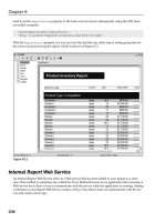
Electrical Power Systems Quality, Second Edition phần 7 pdf
Bạn đang xem bản rút gọn của tài liệu. Xem và tải ngay bản đầy đủ của tài liệu tại đây (286.37 KB, 53 trang )
island. Therefore, some means of direct transfer trip is generally
required to ensure that the generator disconnects from the system
when certain utility breakers operate.
A more normal connection of DG is to use power and power factor
control. This minimizes the risk of islanding. Although the DG no
longer attempts to regulate the voltage, it is still useful for voltage reg-
ulation purposes during constrained loading conditions by displacing
some active and reactive power. Alternatively, customer-owned DG
may be exploited simply by operating off-grid and supporting part or all
of the customer’s load off-line. This avoids interconnection issues and
provides some assistance to voltage regulation by reducing the load.
The controls of distributed sources must be carefully coordinated
with existing line regulators and substation LTCs. Reverse power flow
can sometimes fool voltage regulators into moving the tap changer in
the wrong direction. Also, it is possible for the generator to cause regu-
lators to change taps constantly, causing early failure of the tap-chang-
ing mechanism. Fortunately, some regulator manufacturers have
anticipated these problems and now provide sophisticated microcom-
puter-based regulator controls that are able to compensate.
To exploit dispersed sources for voltage regulation, one is limited in
options to the types of devices with steady, controllable outputs such as
reciprocating engines, combustion turbines, fuel cells, and battery stor-
age. Randomly varying sources such as wind turbines and photo-
voltaics are unsatisfactory for this role and often must be placed on a
relatively stiff part of the system or have special regulation to avoid
voltage regulation difficulties. DG used for voltage regulation must
also be large enough to accomplish the task.
Not all technologies are suitable for regulating voltage. They must be
capable of producing a controlled amount of reactive power.
Manufacturers of devices requiring inverters for interconnection some-
times program the inverter controls to operate only at unity power factor
while grid-connected. Simple induction generators consume reactive
power like an induction motor, which can cause low voltage.
7.7 Flicker*
Although voltage flicker is not technically a long-term voltage varia-
tion, it is included in this chapter because the root cause of problems is
the same: The system is too weak to support the load. Also, some of the
solutions are the same as for the slow-changing voltage regulation
problems. The voltage variations resulting from flicker are often within
the normal service voltage range, but the changes are sufficiently rapid
to be irritating to certain end users.
316 Chapter Seven
*This section was contributed by Jeff W. Smith.
Long-Duration Voltage Variations
Downloaded from Digital Engineering Library @ McGraw-Hill (www.digitalengineeringlibrary.com)
Copyright © 2004 The McGraw-Hill Companies. All rights reserved.
Any use is subject to the Terms of Use as given at the website.
Flicker is a relatively old subject that has gained considerable
attention recently due to the increased awareness of issues concern-
ing power quality. Power engineers first dealt with flicker in the
1880s when the decision of using ac over dc was of concern.
2
Low-fre-
quency ac voltage resulted in a “flickering” of the lights. To avoid this
problem, a higher 60-Hz frequency was chosen as the standard in
North America.
The term flicker is sometimes considered synonymous with voltage
fluctuations, voltage flicker, light flicker, or lamp flicker. The phenom-
enon being referred to can be defined as a fluctuation in system voltage
that can result in observable changes (flickering) in light output.
Because flicker is mostly a problem when the human eye observes it, it
is considered to be a problem of perception.
In the early 1900s, many studies were done on humans to deter-
mine observable and objectionable levels of flicker. Many curves, such
as the one shown in Fig. 7.14, were developed by various companies
to determine the severity of flicker. The flicker curve shown in Fig.
7.14 was developed by C. P. Xenis and W. Perine in 1937 and was
based upon data obtained from 21 groups of observers. In order to
account for the nature of flicker, the observers were exposed to vari-
ous waveshape voltage variations, levels of illumination, and types of
lighting.
3
Long-Duration Voltage Variations 317
1.0
2.0
3.0
4.0
5.0
6.0
7.0
0.1 1.0 10.0 100.0
Frequency of Flicker in Seconds
Voltage Change (in Volts) on 120-V System
T
h
r
e
s
h
o
l
d
o
f
P
e
r
c
e
p
t
i
o
n
T
h
r
e
s
h
o
l
d
o
f
O
b
j
e
c
t
i
o
n
Figure 7.14 General flicker curve.
Long-Duration Voltage Variations
Downloaded from Digital Engineering Library @ McGraw-Hill (www.digitalengineeringlibrary.com)
Copyright © 2004 The McGraw-Hill Companies. All rights reserved.
Any use is subject to the Terms of Use as given at the website.
Flicker can be separated into two types: cyclic and noncyclic. Cyclic
flicker is a result of periodic voltage fluctuations on the system, while
noncyclic is a result of occasional voltage fluctuations.
An example of sinusoidal-cyclic flicker is shown in Fig. 7.15. This
type of flicker is simply amplitude modulation where the main signal
(60 Hz for North America) is the carrier signal and flicker is the modu-
lating signal. Flicker signals are usually specified as a percentage of
the normal operating voltage. By using a percentage, the flicker signal
is independent of peak, peak-to-peak, rms, line-to-neutral, etc.
Typically, percent voltage modulation is expressed by
Percent voltage modulation ϭϫ100%
where V
max
ϭ maximum value of modulated signal
V
min
ϭ minimum value of modulated signal
V
0
ϭ average value of normal operating voltage
The usual method for expressing flicker is similar to that of percent
voltage modulation. It is usually expressed as a percent of the total
change in voltage with respect to the average voltage (⌬V/V) over a cer-
tain period of time.
V
max
Ϫ V
min
ᎏᎏ
V
0
318 Chapter Seven
–200
–150
–100
–50
0
50
100
150
200
0.000
0.058
0.117
0.175
0.233
0.292
0.350
0.408
0.467
0.525
0.583
0.642
0.700
0.758
0.817
0.875
0.933
Time (s)
Voltage (V)
Figure 7.15 Example flicker waveform.
Long-Duration Voltage Variations
Downloaded from Digital Engineering Library @ McGraw-Hill (www.digitalengineeringlibrary.com)
Copyright © 2004 The McGraw-Hill Companies. All rights reserved.
Any use is subject to the Terms of Use as given at the website.
The frequency content of flicker is extremely important in determin-
ing whether or not flicker levels are observable (or objectionable).
Describing the frequency content of the flicker signal in terms of mod-
ulation would mean that the flicker frequency is essentially the fre-
quency of the modulating signal. The typical frequency range of
observable flicker is from 0.5 to 30.0 Hz, with observable magnitudes
starting at less than 1.0 percent.
As shown in Fig. 7.14, the human eye is more sensitive to luminance
fluctuations in the 5- to 10-Hz range. As the frequency of flicker
increases or decreases away from this range, the human eye generally
becomes more tolerable of fluctuations.
One issue that was not considered in the development of the tradi-
tional flicker curve is that of multiple flicker signals. Generally, most
flicker-producing loads contain multiple flicker signals (of varying
magnitudes and frequencies), thus making it very difficult to accu-
rately quantify flicker using flicker curves.
7.7.1 Sources of flicker
Typically, flicker occurs on systems that are weak relative to the
amount of power required by the load, resulting in a low short-circuit
ratio. This, in combination with considerable variations in current over
a short period of time, results in flicker. As the load increases, the cur-
rent in the line increases, thus increasing the voltage drop across the
line. This phenomenon results in a sudden reduction in bus voltage.
Depending upon the change in magnitude of voltage and frequency of
occurrence, this could result in observable amounts of flicker. If a light-
ing load were connected to the system in relatively close proximity to
the fluctuating load, observers could see this as a dimming of the lights.
A common situation, which could result in flicker, would be a large
industrial plant located at the end of a weak distribution feeder.
Whether the resulting voltage fluctuations cause observable or objec-
tionable flicker is dependent upon the following parameters:
■
Size (VA) of potential flicker-producing source
■
System impedance (stiffness of utility)
■
Frequency of resulting voltage fluctuations
A common load that can often cause flicker is an electric arc furnace
(EAF). EAFs are nonlinear, time-varying loads that often cause large
voltage fluctuations and harmonic distortion. Most of the large current
fluctuations occur at the beginning of the melting cycle. During this
period, pieces of scrap steel can actually bridge the gap between the elec-
trodes, resulting in a highly reactive short circuit on the secondary side
Long-Duration Voltage Variations 319
Long-Duration Voltage Variations
Downloaded from Digital Engineering Library @ McGraw-Hill (www.digitalengineeringlibrary.com)
Copyright © 2004 The McGraw-Hill Companies. All rights reserved.
Any use is subject to the Terms of Use as given at the website.
of the furnace transformer. This meltdown period can generally result in
flicker in the 1.0- to 10.0-Hz range. Once the melting cycle is over and the
refining period is reached, stable arcs can usually be held on the elec-
trodes resulting in a steady, three-phase load with high power factor.
4
Large induction machines undergoing start-up or widely varying
load torque changes are also known to produce voltage fluctuations on
systems. As a motor is started up, most of the power drawn by the
motor is reactive (see Fig. 7.16). This results in a large voltage drop
across distribution lines. The most severe case would be when a motor
is started across the line. This type of start-up can result in current
drawn by the motor up to multiples of the full load current.
An example illustrating the impact motor starting and torque changes
can have on system voltage is shown in Fig. 7.17. In this case, a large
industrial plant is located at the end of a weak distribution feeder. Within
the plant are four relatively large induction machines that are frequently
restarted and undergo relatively large load torque variations.
5
Although starting large induction machines across the line is gener-
ally not a recommended practice, it does occur. To reduce flicker, large
motors are brought up to speed using various soft-start techniques
such as reduced-voltage starters or variable-speed drives.
In certain circumstances, superimposed interharmonics in the sup-
ply voltage can lead to oscillating luminous flux and cause flicker.
Voltage interharmonics are components in the harmonic spectrum that
are noninteger multiples of the fundamental frequency. This phenom-
enon can be observed with incandescent lamps as well as with fluores-
cent lamps. Sources of interharmonics include static frequency
converters, cycloconverters, subsynchronous converter cascades,
induction furnaces, and arc furnaces.
6
320 Chapter Seven
1.0 0.9 0.8 0.7 0.6 0.5
Slip
0.4 0.3 0.2 0.1 0.0
Active Power
Reactive Power
Q
P
Figure 7.16 Active and reactive power during induction machine
start-up.
Long-Duration Voltage Variations
Downloaded from Digital Engineering Library @ McGraw-Hill (www.digitalengineeringlibrary.com)
Copyright © 2004 The McGraw-Hill Companies. All rights reserved.
Any use is subject to the Terms of Use as given at the website.
7.7.2 Mitigation techniques
Many options are available to alleviate flicker problems. Mitigation
alternatives include static capacitors, power electronic-based switch-
ing devices, and increasing system capacity. The particular method
chosen is based upon many factors such as the type of load causing the
flicker, the capacity of the system supplying the load, and cost of miti-
gation technique.
Flicker is usually the result of a varying load that is large relative to
the system short-circuit capacity. One obvious way to remove flicker
from the system would be to increase the system capacity sufficiently
to decrease the relative impact of the flicker-producing load. Upgrading
the system could include any of the following: reconductoring, replac-
ing existing transformers with higher kVA ratings, or increasing the
operating voltage.
Motor modifications are also an available option to reduce the
amount of flicker produced during motor starting and load varia-
tions. The motor can be rewound (changing the motor class) such
that the speed-torque curves are modified. Unfortunately, in some
cases this could result in a lower running efficiency. Flywheel energy
systems can also reduce the amount of current drawn by motors by
delivering the mechanical energy required to compensate for load
torque variations.
Recently, series reactors have been found to reduce the amount of
flicker experienced on a system caused by EAFs. Series reactors help sta-
bilize the arc, thus reducing the current variations during the beginning
of melting periods. By adding the series reactor, the sudden increase in
current is reduced due the increase in circuit reactance. Series reactors
Long-Duration Voltage Variations 321
Motor Starting and Load Torque Variations
40
60
80
100
120
140
299000 302000 305000 308000 311000 314000
Time (ms)
Figure 7.17 Voltage fluctuations caused by induction machine operation.
Long-Duration Voltage Variations
Downloaded from Digital Engineering Library @ McGraw-Hill (www.digitalengineeringlibrary.com)
Copyright © 2004 The McGraw-Hill Companies. All rights reserved.
Any use is subject to the Terms of Use as given at the website.
also have the benefit of reducing the supply-side harmonic levels.
7
The
design of the reactor must be coordinated with power requirements.
Series capacitors can also be used to reduce the effect of flicker on an
existing system. In general, series capacitors are placed in series with
the transmission line supplying the load. The benefit of series capacitors
is that the reaction time for the correction to load fluctuations is instan-
taneous in nature. The downside to series capacitors is that compensa-
tion is only available beyond the capacitor. Bus voltages between the
supply and the capacitor are uncompensated. Also, series capacitors
have operational difficulties that require careful engineering.
Fixed shunt-connected capacitor banks are used for long-term volt-
age support or power factor correction. A misconception is that shunt
capacitors can be used to reduce flicker. The starting voltage sag is
reduced, but the percent change in voltage (⌬V/V) is not reduced, and
in some cases can actually be increased.
A rather inexpensive method for reducing the flicker effects of motor
starting would be to simply install a step-starter for the motor, which
would reduce the amount of starting current during motor start-up.
With the advances in solid-state technology, the size, weight, and cost
of adjustable-speed drives have decreased, thus allowing the use of
such devices to be more feasible in reducing the flicker effects caused
by flicker-producing loads.
Static var compensators (SVCs) are very flexible and have many
roles in power systems. SVCs can be used for power factor correction,
flicker reduction, and steady-state voltage control, and also have the
benefit of being able to filter out undesirable frequencies from the sys-
tem. SVCs typically consist of a TCR in parallel with fixed capacitors
(Fig. 7.18). The fixed capacitors are usually connected in ungrounded
wye with a series inductor to implement a filter. The reactive power
that the inductor delivers in the filter is small relative to the rating of
the filter (approximately 1 to 2 percent). There are often multiple filter
stages tuned to different harmonics. The controls in the TCR allow con-
tinuous variations in the amount of reactive power delivered to the sys-
tem, thus increasing the reactive power during heavy loading periods
and reducing the reactive power during light loading.
SVCs can be very effective in controlling voltage fluctuations at
rapidly varying loads. Unfortunately, the price for such flexibility is
high. Nevertheless, they are often the only cost-effective solution for
many loads located in remote areas where the power system is weak.
Much of the cost is in the power electronics on the TCR. Sometimes this
can be reduced by using a number of capacitor steps. The TCR then
need only be large enough to cover the reactive power gap between the
capacitor stages.
322 Chapter Seven
Long-Duration Voltage Variations
Downloaded from Digital Engineering Library @ McGraw-Hill (www.digitalengineeringlibrary.com)
Copyright © 2004 The McGraw-Hill Companies. All rights reserved.
Any use is subject to the Terms of Use as given at the website.
Thyristor-switched capacitors (TSCs) can also be used to supply reac-
tive power to the power system in a very short amount of time, thus
being helpful in reducing the effects of quick load fluctuations. TSCs
usually consist of two to five shunt capacitor banks connected in series
with diodes and thyristors connected back to back. The capacitor sizes
are usually equal to each other or are set at multiples of each other,
allowing for smoother transitions and increased flexibility in reactive
power control. Switching the capacitors in or out of the system in dis-
crete steps controls the amount of reactive power delivered to the sys-
tem by the TSC. This action is unlike that of the SVC, where the
Long-Duration Voltage Variations 323
Fixed Capacitors and Tuning Reactors TCR
Fixed Capacitors (Single-Phase)
Tuning
Reactors
5th
Harmonic
7th
Harmonic
11th
Harmonic
13th
Harmonic
High-Pass
Filter
Figure 7.18 Typical SVC configuration.
Long-Duration Voltage Variations
Downloaded from Digital Engineering Library @ McGraw-Hill (www.digitalengineeringlibrary.com)
Copyright © 2004 The McGraw-Hill Companies. All rights reserved.
Any use is subject to the Terms of Use as given at the website.
capacitors are static and the reactors are used to control the reactive
power. An example diagram of a TSC is shown in Fig. 7.19.
The control of the TSC is usually based on line voltage magnitude,
line current magnitude, or reactive power flow in the line. The control
circuits can be used for all three phases or each phase separately. The
individual phase control offers improved compensation when unbal-
anced loads are producing flicker.
7.7.3 Quantifying flicker
Flicker has been a power quality problem even before the term power
quality was established. However, it has taken many years to develop
an adequate means of quantifying flicker levels. Chapter 11 provides
an in-depth look at power quality monitoring, with a section that
describes modern techniques for measuring and quantifying flicker.
7.8 References
1. L. Morgan, S. Ihara, “Distribution Feeder Modification to Service Both Sensitive
Loads and Large Drives,” 1991 IEEE PES Transmission and Distribution Conference
Record, Dallas, September 1991, pp. 686–690.
2. E. L. Owen, “Power Disturbance and Power Quality—Light Flicker Voltage
Requirements,” Conference Record, IEEE IAS Annual Meeting, Denver, October
1994, pp. 2303–2309.
3. C. P. Xenis, W. Perine, “Slide Rule Yields Lamp Flicker Data.” Electrical World, Oct.
23, 1937, p. 53.
4. S. B. Griscom, “Lamp Flicker on Power Systems,” Chap. 22, Electrical Transmission
and Distribution Reference Book, 4th ed., Westinghouse Elec. Corp., East Pittsburgh,
Pa., 1950.
5. S. M. Halpin, J. W. Smith, C. A. Litton, “Designing Industrial Systems with a Weak
Utility Supply,” IEEE Industry Applications Magazine, March/April 2001, pp. 63–70.
6. Interharmonics in Power Systems, IEEE Interharmonic Task Force, Cigre
36.05/CIRED 2 CC02, Voltage Quality Working Group.
7. S. R. Mendis, M. T. Bishop, T. R. Day, D. M. Boyd, “Evaluation of Supplementary
Series Reactors to Optimize Electric Arc Furnace Operations,” Conference Record,
IEEE IAS Annual Meeting, Orlando, Fla., October 1995, pp. 2154–2161.
324 Chapter Seven
Figure 7.19 Typical TSC configuration.
Long-Duration Voltage Variations
Downloaded from Digital Engineering Library @ McGraw-Hill (www.digitalengineeringlibrary.com)
Copyright © 2004 The McGraw-Hill Companies. All rights reserved.
Any use is subject to the Terms of Use as given at the website.
7.9 Bibliography
IEEE Standard 141-1993: Recommended Practice for Power Distribution in Industrial
Plants, IEEE, 1993.
IEEE Standard 519-1992: Recommended Practices and Requirements for Harmonic
Control in Electrical Power Systems, IEEE, 1993.
IEC 61000-4-15, Electromagnetic Compatibility (EMC). Part 4: Testing and Measuring
Techniques. Section 15: Flickermeter—Functional and Design Specifications.
Long-Duration Voltage Variations 325
Long-Duration Voltage Variations
Downloaded from Digital Engineering Library @ McGraw-Hill (www.digitalengineeringlibrary.com)
Copyright © 2004 The McGraw-Hill Companies. All rights reserved.
Any use is subject to the Terms of Use as given at the website.
Long-Duration Voltage Variations
Downloaded from Digital Engineering Library @ McGraw-Hill (www.digitalengineeringlibrary.com)
Copyright © 2004 The McGraw-Hill Companies. All rights reserved.
Any use is subject to the Terms of Use as given at the website.
327
Power Quality Benchmarking
Foreword EPRI has been studying power quality (PQ) problems and
solutions for over 15 years. This chapter presents many new and
innovative approaches to PQ monitoring, analysis, and planning that
have been developed since the First Edition of this book. The authors
have been intimately involved in this research. Tremendous progress
has been made and readers can gain a better understanding of the
state-of-the-art of this research, which continues.
Power quality benchmarking is an important aspect in the overall
structure of a power quality program. The benchmarking process begins
with defining the metrics to be used for benchmarking and evaluating
service quality. The EPRI Reliability Benchmarking Methodology
project (EPRI Reliability Benchmarking Methodology, EPRI TR-
107938, EPRI, Palo Alto, California) defined a set of PQ indices that
serve as metrics for quantifying quality of service. These indices are
calculated from data measured on the system by specialized
instrumentation. Many utilities around the world have implemented
permanent PQ monitoring systems for benchmarking power quality.
However, there are still considerably large gaps in coverage of the power
system with PQ monitors. As part of the EPRI Reliability
Benchmarking Methodology project, investigators explored the idea of
estimating the voltages at locations without monitors given the data at
only one monitor or a few monitors. This resulted in the development of
the concept of the EPRI Power Quality State Estimator (PQSE), which
uses feeder models and recorded data to estimate what would have been
recorded on the customer side of the service transformer.
This chapter will serve as a useful reference for identifying suitable
indices for benchmarking the quality of service and analytical methods
for extending the capabilities of PQ monitoring instrumentation. We
Chapter
8
Downloaded from Digital Engineering Library @ McGraw-Hill (www.digitalengineeringlibrary.com)
Copyright © 2004 The McGraw-Hill Companies. All rights reserved.
Any use is subject to the Terms of Use as given at the website.
Source: Electrical Power Systems Quality
applaud the authors for presenting this information in an easily
understandable manner. In the overall context of a PQ program,
benchmarking is an essential ingredient.
Ashok Sundaram, EPRI
Arshad Mansoor, EPRI-PEAC Corporation
8.1 Introduction
Because of sensitive customer loads, there is a need to define the qual-
ity of electricity provided in a common and succinct manner that can be
evaluated by the electricity supplier as well as by consumers or equip-
ment suppliers. This chapter describes recent developments in meth-
ods for benchmarking the performance of electricity supply.
One of the basic tenets of solving power quality problems is that dis-
turbances in the electric power system are not restricted by legal
boundaries. Power suppliers, power consumers, and equipment suppli-
ers must work together to solve many problems. Before they can do
that, they must understand the electrical environment in which end-
use equipment operates. This is necessary to reduce the long-term eco-
nomic impact of inevitable power quality variations and to identify
system improvements that can mitigate power quality problems.
1–3
A comprehensive set of power quality indices was defined for the
Electric Power Research Institute (EPRI) Reliability Benchmarking
Methodology (RBM) project
1
to serve as metrics for quantifying quality
of service. The power quality indices are used to evaluate compatibility
between the voltage as delivered by the electric utility and the sensi-
tivity of the end user’s equipment. The indices were patterned after the
indices commonly used by utilities to describe reliability to reduce the
learning curve. A few of the indices have become popular, and software
has been developed to compute them from measured data and estimate
them from simulations. We will examine the definitions of some of the
indices and then look at how they might be included in contracts and
planning.
8.2 Benchmarking Process
Electric utilities throughout the world are embracing the concept of
benchmarking service quality. Utilities realize that they must under-
stand the levels of service quality provided throughout their distribu-
tion systems and determine if the levels provided are appropriate. This
is certainly becoming more prevalent as more utilities contract with
specific customers to provide a specified quality of service over some
period of time. The typical steps in the power quality benchmarking
process are
328 Chapter Eight
Power Quality Benchmarking
Downloaded from Digital Engineering Library @ McGraw-Hill (www.digitalengineeringlibrary.com)
Copyright © 2004 The McGraw-Hill Companies. All rights reserved.
Any use is subject to the Terms of Use as given at the website.
1. Select benchmarking metrics. The EPRI RBM project defined sev-
eral performance indices for evaluating the electric service quality.
4
A select group are described here in more detail.
2. Collect power quality data. This involves the placement of power
quality monitors on the system and characterization of the perfor-
mance of the system. A variety of instruments and monitoring sys-
tems have been recently developed to assist with this
labor-intensive process (see Chap. 11).
3. Select the benchmark. This could be based on past performance, a
standard adopted by similar utilities, or a standard established by a
professional or standards organization such as the IEEE, IEC,
ANSI, or NEMA.
4. Determine target performance levels. These are targets that are
appropriate and economically feasible. Target levels may be limited
to specific customers or customer groups and may exceed the bench-
mark values.
The benchmarking process begins with selection of the metrics to be
used for benchmarking and evaluating service quality. The metrics
could simply be estimated from historical data such as average number
of faults per mile of line and assuming the fault resulted in a certain
number of sags and interruptions. However, electricity providers and
consumers are increasingly interested in metrics that describe the
actual performance for a given time period. The indices developed as
part of the EPRI RBM project are calculated from data measured on
the system by specialized instrumentation.
Electric utilities throughout the world are deploying power quality
monitoring infrastructures that provide the data required for accurate
benchmarking of the service quality provided to consumers. These are
permanent monitoring systems due to the time needed to obtain accu-
rate data and the importance of power quality to the end users where
these systems are being installed. For most utilities and consumers,
the most important power quality variation is the voltage sag due to
short-circuit faults. Although these events are not necessarily the most
frequent, they have a tremendous economic impact on end users. The
process of benchmarking voltage sag levels generally requires 2 to 3
years of sampling. These data can then be quantified to relate voltage
sag performance with standardized indices that are understandable by
both utilities and customers.
Finally, after the appropriate data have been acquired, the service
provider must determine what levels of quality are appropriate and
economically feasible. Increasingly, utilities are making these decisions
in conjunction with individual customers or regulatory agencies. The
Power Quality Benchmarking 329
Power Quality Benchmarking
Downloaded from Digital Engineering Library @ McGraw-Hill (www.digitalengineeringlibrary.com)
Copyright © 2004 The McGraw-Hill Companies. All rights reserved.
Any use is subject to the Terms of Use as given at the website.
economic law of diminishing returns applies to increasing the quality
of electricity as it applies to most quality assurance programs. Electric
utilities note that nearly any level of service quality can be achieved
through alternate feeders, standby generators, UPS systems, energy
storage, etc. However, at some point the costs cannot be economically
justified and must be balanced with the needs of end users and the
value of service to them.
Most utilities have been benchmarking reliability for several
decades. In the context of this book, reliability deals with sustained
interruptions. IEEE Standard 1366-1998 was established to define the
benchmarking metrics for this area of power quality.
5
The metrics are
defined in terms of system average or customer average indices regard-
ing such things as the number of interruptions and the duration of
interruption (SAIDI, SAIFI, etc.). However, the reliability indices do
not capture the impact of loads tripping off-line for 70 percent voltage
sags nor the loss of efficiency and premature equipment failure due to
excessive harmonic distortion.
Interest in expanding the service quality benchmarking into areas
other than traditional reliability increased markedly in the late 1980s.
This was largely prompted by experiences with power electronic loads
that produced significant harmonic currents and were much more sensi-
tive to voltage sags than previous generations of electromechanical
loads. In 1989, the EPRI initiated the EPRI Distribution Power Quality
(DPQ) Project, RP 3098-1, to collect power quality data for distribution
systems across the United States. Monitors were placed at nearly 300
locations on 100 distribution feeders, and data were collected for 27
months. The DPQ database contains over 30 gigabytes of power quality
data and has served as the basis for standards efforts and many stud-
ies.
1,6
The results were made available to EPRI member utilities in 1996.
Upon completion of the DPQ project in 1995, it became apparent that
there was no uniform way of benchmarking the performance of specific
service quality measurements against these data. In 1996, the EPRI
completed the RBM project, which provided the power quality indices
to allow service quality to be defined in a consistent manner from one
utility to another.
4
The indices were patterned after the traditional reli-
ability indices with which utility engineers had already become com-
fortable. Indices were defined for
1. Short-duration rms voltage variations. These are voltage sags,
swells, and interruptions of less than 1 min.
2. Harmonic distortion.
3. Transient overvoltages. This category is largely capacitor-switching
transients, but could also include lightning-induced transients.
330 Chapter Eight
Power Quality Benchmarking
Downloaded from Digital Engineering Library @ McGraw-Hill (www.digitalengineeringlibrary.com)
Copyright © 2004 The McGraw-Hill Companies. All rights reserved.
Any use is subject to the Terms of Use as given at the website.
4. Steady-state voltage variations such as voltage regulation and
phase balance.
This chapter describes methodologies for determining target levels of
quality for various applications based on the statistical distribution of
quality indices values calculated from actual measurement data. We
will concentrate on the more popular indices for rms voltage variations
and harmonics. Readers are referred to the documents cited in the ref-
erences to this chapter for more details.
8.3 RMS Voltage Variation Indices
For many years, the only indices defined to quantify rms variation ser-
vice quality were the sustained interruption indices (SAIFI, CAIDI,
etc.). Sustained interruptions are in fact only one type of rms variation.
IEEE Standard 1159-1995
7
defines a sustained interruption as a reduc-
tion in the rms voltage to less than 10 percent of nominal voltage for
longer than 1 min (see Chap. 2).
Sustained interruptions are of great importance because all cus-
tomers on the faulted section are affected by such disturbances.
Indices for evaluating them have been in use informally by utilities for
many years and were recently standardized by the IEEE in IEEE
Standard 1366-1998.
5
Long before, some utilities had been required to
report certain indices to regulatory agencies. The standard also
defines indices quantifying momentary interruption performance,
which quantifies another very important type of rms voltage variation.
Momentary interruptions are due to clearing of temporary faults and
the subsequent reclose operation (see Chap. 3). While they are not cap-
tured in the traditional reliability indices, they affect many end-user
classes. The rms voltage variation indices take this one step farther
and define metrics for voltage sags, which can also affect many end
users adversely.
8.3.1 Characterizing rms variation events
IEEE Standard 1159-1995
7
provides a common terminology that can be
used to discuss and assess rms voltage variations, defining magnitude
ranges for sags, swells, and interruptions. The standard suggests that
the terms sag, swell, and interruption be preceded by a modifier
describing the duration of the event (instantaneous, momentary, tem-
porary, or sustained). These definitions are summarized in Chap. 2.
RMS variations are classified by the magnitude and duration of the
disturbances. Therefore, before rms variation indices can be calculated,
magnitude and duration characteristics must be extracted from the
Power Quality Benchmarking 331
Power Quality Benchmarking
Downloaded from Digital Engineering Library @ McGraw-Hill (www.digitalengineeringlibrary.com)
Copyright © 2004 The McGraw-Hill Companies. All rights reserved.
Any use is subject to the Terms of Use as given at the website.
332 Chapter Eight
raw waveform data recorded for each event. Characterization is a term
used to describe the process of extracting from a measurement useful
pieces of information which describe the event so that not every detail
of the event has to be retained.
Characterization of rms variations can be very complicated. It is
structured into three levels, each of which is identified as a type of
event as follows:
1. Phase or component event
2. Measurement event
3. Aggregate event
Component event level. Each phase of each rms variation measure-
ment may contain multiple components. Most rms variations have a
simple rectangular shape and are accurately characterized by a single
magnitude and duration. Approximately 10 percent of rms variations
are nonrectangular
1
and have multiple components. Consider the rms
variation shown in Fig. 8.1. It exhibits a voltage swell followed by two
levels of voltage sag. This event was the result of clearing a temporary
single-line-to-ground fault that evolved into a double-line-to-ground
Phase A Voltage
RMS Variation
February 20, 1994 at 12:52:52 Local
Trigger
0
20
40
60
80
100
120
140
% Volts
% Volts
–150
–100
–50
0
50
100
150
0
0 25 50 75 100 125 150 175 200
0.25 0.5 0.75 1 1.25 1.5 1.75 2
Time (s)
Time (ms)
Duration
0.633 s
Min 0.166
Ave 75.50
Max 138.8
Ref Cycle
43760
Figure 8.1 Multicomponent, nonrectangular rms variation.
Power Quality Benchmarking
Downloaded from Digital Engineering Library @ McGraw-Hill (www.digitalengineeringlibrary.com)
Copyright © 2004 The McGraw-Hill Companies. All rights reserved.
Any use is subject to the Terms of Use as given at the website.
Power Quality Benchmarking 333
fault before the breaker tripped. The breaker then reclosed successfully
in about 0.2 s. Note that only about 10 cycles of the initial voltage swell
are shown in the waveform plot on the bottom. The entire event lasted
nearly 1.5 s, although the instrument reports only the duration of the
voltage swell. Other software is required to postprocess the waveform
off-line to determine the other characteristics of this event. Variations
like this are much more difficult to characterize because no single mag-
nitude-duration pair completely represents the phase measurement.
Most of the methods for characterization agree that the magnitude
reported must be the maximum deviation from nominal voltage. The dif-
ficulty lies in assigning a duration associated with the magnitude. The
method defined here is called the specified voltage method. This method
designates the duration as the period of time that the rms voltage exceeds
a specified threshold voltage level used to characterize the disturbance.
Thus, events like the one in Fig. 8.1 would be assigned different dura-
tion values depending on the specified voltage threshold of interest.
Figure 8.2 illustrates this concept for three voltage levels: 80, 50, and 10
percent. T
80%
is the duration of the event for an assessment of sags hav-
ing magnitudes Յ80 percent. Likewise, T
50%
and T
10%
are the durations
associated with sags of the corresponding voltage levels. Notice that
T
80%
and T
50%
are both 800 ms because both of the sag components of this
nonrectangular event have magnitudes well below 50 percent. T
10%
,
however, comprises only the duration of the second component, 200 ms.
0
20
40
60
80
100
120
140
0.000 0.167 0.333 0.500 0.667 0.833 1.000 1.167 1.333 1.500 1.667
Time (s)
% Volts
Measurement
Event #1
T
10%
T
50%
T
80%
Figure 8.2 Illustration of specified voltage characterization of rms variation phase mea-
surements.
Power Quality Benchmarking
Downloaded from Digital Engineering Library @ McGraw-Hill (www.digitalengineeringlibrary.com)
Copyright © 2004 The McGraw-Hill Companies. All rights reserved.
Any use is subject to the Terms of Use as given at the website.
Measurement event level. A power system occurrence such as a fault
can affect one, two, or all three phases of the distribution system. The
magnitude and duration of the resulting rms variation may differ sub-
stantially for different phases. A determination must be made concern-
ing how to report three-phase measurement events. For an assessment
of single-phase performance, each of the three phases are reported sep-
arately. Thus, for some faults, three different rms variations are
included in the indices. This will be inappropriate for loads that see
this as a single event.
The method defined here for characterizing measurement events is a
three-phase method. A single set of characteristics are determined for
all affected phases. For each rms variation event, the magnitude and
duration are designated as the magnitude and duration of the phase
with the greatest voltage deviation from nominal voltage.
Aggregate event level. An aggregate event is the collection of all mea-
surements associated with a single power system occurrence into a sin-
gle set of event characteristics. For example, a single distribution system
fault might result in several measurements as the overcurrent protec-
tion system operates to clear the faults and restore service. An aggregate
event associated with this fault would summarize all the associated mea-
surements into a single set of characteristics (magnitude, duration, etc.).
While there may be many individual events, many end-user devices will
trip or misoperate on the initial event. The succeeding rms variations
have no further adverse effect on the end-user process. Thus, aggrega-
tion provides a truer assessment of service quality. RMS variation per-
formance indices are usually based on aggregate events.
A good method of aggregating measurements is to consider all events
that occur within a defined interval of the first event to be part of the
same aggregate event. One minute is a typical time interval, which cor-
responds to the minimum length of a sustained interruption. The mag-
nitude and duration of the aggregate event are determined from the
measurement event most likely to result in customer equipment failure.
This will generally be the event exhibiting the greatest voltage deviation.
8.3.2 RMS variation performance indices
The rms variation indices are designed to assess the service quality for a
specified circuit area. The indices may be scaled to systems of different
sizes. They may be applied to measurements recorded across a utility’s
entire distribution system resulting in SAIFI-like system averages, or the
indices may be applied to a single feeder or a single customer PCC.
There are many properties of rms variations that could be useful to
quantify—properties such as the frequency of occurrence, the duration of
334 Chapter Eight
Power Quality Benchmarking
Downloaded from Digital Engineering Library @ McGraw-Hill (www.digitalengineeringlibrary.com)
Copyright © 2004 The McGraw-Hill Companies. All rights reserved.
Any use is subject to the Terms of Use as given at the website.
disturbances, and the number of phases involved. Many rms variation
indices were defined in the EPRI RBM project to address these various
issues. Space does not permit a description of all of these, so we will con-
centrate on one index that has, perhaps, become the most popular. The
papers and reports included in the references contain details on others.
System average rms (variation) frequency index
Voltage
(SARFI
x
). SARFI
x
represents the average number of specified rms variation measure-
ment events that occurred over the assessment period per customer
served, where the specified disturbances are those with a magnitude
less than x for sags or a magnitude greater than x for swells:
SARFI
x
ϭ
where x ϭ rms voltage threshold; possible values are 140, 120, 110, 90,
80, 70, 50, and 10
N
i
ϭ number of customers experiencing short-duration volt-
age deviations with magnitudes above X percent for X Ͼ
100 or below X percent for X Ͻ 100 due to measurement
event i
N
T
ϭ total number of customers served from section of system to
be assessed
Notice that SARFI is defined with respect to the voltage threshold x.
For example, if a utility has customers that are only susceptible to sags
below 70 percent of nominal voltage, this disturbance group can be
assessed using SARFI
70
. The eight defined threshold values for the
index are not arbitrary. They are chosen to coincide with the following:
140, 120, and 110. Overvoltage segments of the ITI curve.
90, 80, and 70. Undervoltage segments of ITI curve.
50. Typical break point for assessing motor contactors.
10. IEEE Standard 1159 definition of an interruption.
An increasing popular use of SARFI is to define the threshold as a
curve. For example, SARFI
ITIC
would represent the frequency of rms
variation events outside the ITI curve voltage tolerance envelope.
Three such curve indices are commonly computed:
SARFI
CBEMA
SARFI
ITIC
SARFI
SEMI
∑ N
i
ᎏ
N
T
Power Quality Benchmarking 335
Power Quality Benchmarking
Downloaded from Digital Engineering Library @ McGraw-Hill (www.digitalengineeringlibrary.com)
Copyright © 2004 The McGraw-Hill Companies. All rights reserved.
Any use is subject to the Terms of Use as given at the website.
This group of indices is similar to the System Average Interruption
Frequency Index (SAIFI) value that many utilities have calculated for
years. SARFI
x
, however, assesses more than just interruptions. The
frequency of occurrence of rms variations of varying magnitudes can be
assessed using SARFI
x
. Note that SARFI
x
is defined for short-duration
variations as defined by IEEE Standard 1159.
There are three additional indices that are subsets of SARFI
x
. These
indices assess variations of a specific IEEE Standard 1159 duration
category:
1. System Instantaneous Average RMS (Variation) Frequency Index
(SIARFI
x
).
2. System Momentary Average RMS (Variation) Frequency Index
(SMARFI
x
).
3. System Temporary Average RMS (Variation) Frequency Index
(STARFI
x
).
8.3.3 SARFI for the EPRI DPQ project
Table 8.1 shows the statistics for various forms of SARFI computed
for the measurements taken by the EPRI DPQ project. These partic-
ular values are rms variation frequencies for substation sites in num-
ber of events per 365 days. One-minute temporal aggregation was
used, and the data were treated using sampling weights. This can
serve as a reference benchmark for distribution systems in the United
States.
8.3.4 Example index computation
procedure
This example is based on actual data recorded on one of the feeders
monitored during the EPRI DPQ project.
1
This illustrates some of the
practical issues involved in computing the indices.
336 Chapter Eight
SARFI
90
SARFI
80
SARFI
70
SARFI
50
SARFI
10
SARFI
CBEMA
SARFI
ITIC
SARFI
SEMI
Minimum 0.000 0.000 0.000 0.000 0.000 0.000 0.000 0.000
CP05† 11.887 5.594 0.000 0.000 0.000 5.316 2.791 2.362
CP50† 43.987 22.813 12.126 5.165 1.525 25.465 18.765 13.619
Mean 56.308 28.729 18.422 8.926 3.694 33.293 25.390 18.535
CP95† 135.185 66.260 51.000 27.037 13.519 71.413 51.500 38.238
Maximum 207.644 103.405 70.535 56.311 35.689 149.488 140.768 140.768
*Submitted for IEEE Standard P1564.
8
†CP05, CP50, and CP95 are abbreviations that indicate that the value exceeds 5, 50, and 95 percent of the sam-
ples in the database. For example, 50 percent of the sites in the project had more than 18.765 events per year that
were outside the ITI curve voltage tolerance envelope (SARFI
ITIC
).
TABLE 8.1 SARFI Statistics from the EPRI DPQ Project*
Power Quality Benchmarking
Downloaded from Digital Engineering Library @ McGraw-Hill (www.digitalengineeringlibrary.com)
Copyright © 2004 The McGraw-Hill Companies. All rights reserved.
Any use is subject to the Terms of Use as given at the website.
First, one must know how many customers experience a voltage
exceeding the index threshold for each rms variation that occurs.
Obviously, every customer will not be individually monitored.
Consequently, one must approximate the voltage experienced by each
customer during a disturbance. This is accomplished by segmenting
the circuit into small areas across which all customers are assumed to
experience the same voltage. Obviously, the smaller the segments, the
better the approximation.
One method of determining voltages for many circuit segments based
on a limited number of monitoring points is power quality state esti-
mation. A special section (8.7) is included on this topic later. State esti-
mation provides pseudomeasurements for those segments not
containing a measuring instrument. Such state estimation requires a
moderately detailed circuit model and known monitored data. Without
the pseudomeasurements provided by state estimation, the number of
physical monitoring locations becomes the number of constant-voltage
segments upon which the indices that are calculated. This is referred
to as monitor-limited segmentation (MLS) and results in only a few seg-
ments per circuit. Although the calculated index values are less accu-
rate, MLS still yields indices that are informative.
Figure 8.3 illustrates the three MLS segments for the example cal-
culation feeder corresponding to the three power quality monitors, M1,
M2, and M3. The exact number of customers served from each MLS
Power Quality Benchmarking 337
Figure 8.3 Circuit for example rms varia-
tion calculation.
Power Quality Benchmarking
Downloaded from Digital Engineering Library @ McGraw-Hill (www.digitalengineeringlibrary.com)
Copyright © 2004 The McGraw-Hill Companies. All rights reserved.
Any use is subject to the Terms of Use as given at the website.
segment was not available, so values of 500, 100, and 400 were
assumed for segments 1, 2, and 3, respectively, based on the load. With
these assumptions, 1 year of monitoring data yielded the results sum-
marized in Table 8.2.
The sag indices are typical of what would be expected. The number
of customer disturbances decrease as the voltage threshold decreases.
There were very few voltage swells on this feeder. The total number of
sags per customer is estimated at 27.5 per year. Of these, only 7.3 are
below 70 percent and 4.8 are below 50 percent. These two levels are
typically where end users begin to experience problems, and utilities
that use these indices typically set benchmark targets close to these
values.
The SARFI
10
value of 4.3 cannot be compared to SAIFI because
SAIFI reflects only sustained interruptions. The duration-based
indices—SIARFI, SMARFI, and STARFI—are also quite interesting.
The majority of the disturbances are classified as instantaneous by
IEEE Standard 1159. Only 4.8 of the 27.5 sag disturbances are either
momentary or temporary. However, these tend to be the more severe
sags (magnitude of 50 percent and less).
8.3.5 Utility applications
Utilities are using the discussed rms variation indices to improve their
systems.
9
One productive use of the indices is to compute the separate
indices for individual substations as well as the system index for sev-
eral substations. The individual substation values are then compared
to the system value. Those substations that exhibit significantly poor
performance as compared to the system performance are targeted for
maintenance efforts. Based on the sensitivity and needs of the cus-
tomers served from the targeted substations, the economic viability of
potential mitigating actions is assessed. The indices have also proven
338 Chapter Eight
TABLE 8.2 Example RMS Variation Index Values
Calculated for Circuit of Fig. 8.3 Based on 1 Year
of Actual Monitored Data
x SARFI
x
SIARFI
x
SMARFI
x
STARFI
x
140 0.0 0.0 0.0 0.0
120 0.0 0.0 0.0 0.0
110 0.5 0.5 0.0 0.0
90 27.5 22.7 4.3 0.5
80 13.6 8.8 4.3 0.5
70 7.3 2.5 4.3 0.5
50 4.8 0.5 3.8 0.5
10 4.3 Undefined 3.8 0.5
Power Quality Benchmarking
Downloaded from Digital Engineering Library @ McGraw-Hill (www.digitalengineeringlibrary.com)
Copyright © 2004 The McGraw-Hill Companies. All rights reserved.
Any use is subject to the Terms of Use as given at the website.
to be excellent tools for communicating performance of the power deliv-
ery system in a simplified manner to key industrial customers.
8.4 Harmonics Indices
Power electronic devices offer electrical efficiencies and flexibility but
present a double-edged coordination problem with harmonics. Not only
do they produce harmonics, but they also are typically more sensitive
to the resulting distortion than more traditional electromechanical
load devices. End users expecting an improved level of service may
actually experience more problems. This section discusses power qual-
ity indices for assessing the quality of service with respect to harmonic
voltage distortion. Before we get into the definition of the indices, some
issues regarding sampling are discussed.
8.4.1 Sampling techniques
Power quality engineers typically configure power quality monitors to
periodically record a sample of voltage and current for each of the three
phases and the neutral. The measurements typically consist of a single
cycle, but longer samples may be needed to capture such phenomena as
interharmonics. The power quality monitors take samples at intervals
of 15 to 30 min and record thousands of measurements that are sum-
marized by the indices. Besides harmonic distortion, the recorded
waveforms yield information about other steady-state characteristics
such as phase unbalance, power factor, form factor, and crest factor. We
will focus here on harmonic content.
The fundamental quantity used to form the indices is the THD of the
voltage. The definition of THD may be found in Chap. 5 and is repeated
here in Eq. (8.1):
V
THD
ϭ (8.1)
Voltage distortion is not a constant value. On a typical system, the
harmonic distortion follows daily, weekly, and seasonal patterns. An
example of daily patterns of total harmonic voltage distortion for 1 week
is shown in Fig. 8.4. This is typical for many residential feeders where
the voltage distortion is highest late at night when the load is low.
A useful method of summarizing the THD samples of trends like that
in Fig. 8.4 is to create a histogram like that shown in Fig. 8.5. Note the
two distinct peaks in the distribution, which reflects the bimodal
nature of the harmonic distortion trend.
Ί
Α
∞
h ϭ 2
V
h
2
ᎏᎏ
V
1
Power Quality Benchmarking 339
Power Quality Benchmarking
Downloaded from Digital Engineering Library @ McGraw-Hill (www.digitalengineeringlibrary.com)
Copyright © 2004 The McGraw-Hill Companies. All rights reserved.
Any use is subject to the Terms of Use as given at the website.
Once the histogram is prepared, the cumulative frequency curve is
computed. This is shown overlaying the histogram in Fig. 8.5 and has
been pulled out separately in Fig. 8.6 to demonstrate the computation of
the 95th percentile value, known as CP95. In this example, a voltage
THD of 3.17 percent is larger than 95 percent of all other samples in the
distribution. CP95 is frequently more valuable than the maximum value
of a distribution because it is less sensitive to spurious measurements.
Usually an electric utility will collect measurements at more than
one location and compute a different CP95 value for each monitoring
location. Figure 8.7 shows a histogram of CP95 values compiled from
different sites, which serves to summarize the measurements both
340 Chapter Eight
0%
1%
2%
3%
4%
5/1/95 5/3/95 5/5/95 5/7/95 5/9/95
V
THD
Figure 8.4 Trend of voltage total harmonic distortion demonstrat-
ing daily cycle for 1 week.
0
50
100
150
200
250
300
0.0%
0.4%
0.8%
1.2%
1.6%
2.0%
2.4%
2.8%
3.2%
3.6%
4.0%
0%
10%
20%
30%
40%
50%
60%
70%
80%
90%
100%
Cumulative Frequency
Count of Samples
V
THD
Figure 8.5 Histogram of voltage total harmonic distortion for 1 month
demonstrating bimodal distribution.
Power Quality Benchmarking
Downloaded from Digital Engineering Library @ McGraw-Hill (www.digitalengineeringlibrary.com)
Copyright © 2004 The McGraw-Hill Companies. All rights reserved.
Any use is subject to the Terms of Use as given at the website.