In air X
N
2
/X
O
2
= 3.76. Furthermore,
(X
O
2( )l
/X
N
2( )l
) = (X
O
2
/X
N
2
)/(
P
N
sat
2
(T)/
P
O
sat
2
(T)) (C)
Since

P
N
sat
2
(T) ≈
P
O
sat
2
(T),
(X
O
2( )l
/X
N
2( )l
) = (X
O
2
/X
N
2
) = 3.76.
Remarks
As the temperature rises, the value of
P
k
sat
for a substance increases. Hence X
k,

l
de-
creases. The warming of river water decreases the O
2
and N
2
concentrations in it.
j. Example 10
cuss the effects with salt addition at 111.4ºC.
Solution
P
sat
(111.4ºC) = 1.5 bar. The total volume
V = m
g
v
g
+ m
f
v
f
= m (x v
g
+ (1–x) v
f
) (A)
= m (0.2× 1.159 +0.8× 0.001053) = m (0.233).
Therefore,
m = 20×0.001/0.233 = 0.0858 kg
Using the ideal gas law for the vapor phase

m = V
f
/v
f
+ (V – V
f
)/(RT/P
o
), (B)
V
f
= (m – P
o
V/RT)/(1/v
f
– P
o
/RT) ≈ v
f
(m – P
o
V/RT). (C)
The pressure increases as additional gas is injected, thereby increasing the Gibbs en-
ergy of the liquid and vapor phases.
In case of liquid water,
g
l
(T,P) = g
l
(T,P

sat
) + v
l
(P – P
sat
).
For an ideal gas mixture in the vapor phase,
ˆ
g
HO
2
(T,P,X
H2O
) =
g
HO
2
(T,p
HO
2
) =
g
H2O
(T,P
sat
) + ∫
v
H2O(g)
dP
=

g
g
(T,P
sat
) +
R
T ln(p
HO
2
/P
sat
). (D)
Equating Eq. ( C) with Eq. (D)
v
(P – P
sat
) = RT ln (p
HO
2
/P
sat
), or ln(p
HO
2
/P
sat
) = (v
l
(P – P
sat

))/(RT) (E)
This relation is known as the Kelvin–Helmholtz formula which shows the effect of
total pressure on partial pressure of vapor. Note that the partial pressure of H
2
O in the
vapor phase is not the same as saturation pressure at T.
For water, v
l
= 0.001053 m
3
kmole
–1
, P
sat
= 1.5 bar, and for this case P = 2 bar, and T
= 384.56 K. Therefore, the partial pressure of H
2
O in vapor phase,
p
HO
2
= 1.500445 bar.
a value close to saturation pressure at T= 384.6K since v
f
is small. Further
A 20-liter rigid volume consists of 80% liquid and 20% vapor by mass at 111.4ºC and
1.5 bar. A pin is placed on piston to prevent its motion. Gaseous nitrogen is isother-
mally injected into the volume until the pressure reaches 2 bar. What is the nitrogen
mole fraction in the gas phase? Assume that N
2

does not dissolve in the liquid.
What happens if there is no pin during the injection of N
2
. Instead of adding N
2
, dis-
X
HO
2
= 0.75022, and X
N2
= 0.24798.
The vapor mass
m
v
= p
v
V
v
/RT = p
v
(V – V
f
)/RT, and
the liquid mass
m
f
= V
f
/v

f
.
Adding the two masses,
m = p
v
(V – V
f
)/RT + V
f
/v
f
.
Therefore,
V
f
= (m – p
v
V/RT)/(1/v
f
– p
v
/RT) ≈ v
f
(m – p
v
V/RT). (F)
Since P
v
after N
2

injection is slightly higher than P
v
before N
2
injection, there should
be more vapor; thus the volume of liquid decreases. According to Le Chatelier, the
system counteracts the pressure increase by increasing the volume of the vapor phase.
If we ignore the term (v
f
(P – P
sat
))/(RT), in Eq. (A) this implies that p
H2O
= P
sat
and X
v
= 0.75.
The injection of nitrogen implies that X
H2O
<1. Pressure remains constant. Therefore,
)
g
HO
2
=
g
HO
2
(T,P) +

R
T ln X
H2O
. Since X
H2O
<1,
)
g
HO
2
<
)
l
g
HO
2
()
(T,P), as long as the
temperature and pressure are maintained, vaporization continues until all of the liquid
vaporizes.
Similarly when we add salt in water( or an impurity), the Gibbs function of the liquid
H
2
O decreases which causes the vapor molecules to cross over from the vapor into the
liquid phase.
Remarks
At a specified temperature, an increase in pressure causes the "g" of liquid to increase
slightly. The Gibbs free energy of the vapor equals that of the liquid. If the vapor is
an ideal gas, the enthalpy of the vapor will remain unchanged. The slight Gibbs en-
0

0.05
0.1
0.15
0.2
0.25
0.3
0.35
0.4
0.45
300 350 400 450 500 550
T, K
X
2
0
0.2
0.4
0.6
0.8
1
1.2
X
1
Figure 7: The variation of the mole fraction of heptane vapor with droplet temperature
for a mixture containing 60 % n–heptane and 40 % hexadecane at 100 kPa.
ergy increase must then cause the entropy of vapor to decrease which corresponds to
an increase in the partial pressure of vapor.
Consider a component k of a liquid mixture that exists in equilibrium with a vapor
phase that also contains a mixture of insoluble inert gases. In this case,
µ
k(l)

(T,P) = µ
k(g)
(T, P).
If the vapor phase is isothermally pressurized, then
µ
k(l)
(T,P) + dµ
k(l)
= µ
k(g)
(T,P) + dµ
k(g(
, v
k(l)
dP
l
= v
k(g)
dP
g
and dP
l
/dP
g
= v
k
g
/v
k
l

.
An increase in the pressure in the vapor phase requires a large change in the liquid
phase pressure to ensure that liquid–vapor equilibrium is maintained.
2. Immiscible Mixture
a. Immiscible Liquids and Miscible Gas Phase
This case is illustrated through the following example.
k. Example 11
pressure and temperature. You may assume that
ln
P
sat
2
= 13.97 – 5205.2/T (K), and (A)
ln
P
sat
1
= 13.98 – 4719.2/T (K). (B)
Solution
Employing Eqs. (A) and (B), the normal boiling points of species 1 (methanol) and 2
(water) are, respectively, 64.4 and 100ºC.
We will employ Raoult’s Law, in which the liquid mole fractions for water and
methanol must be set to unity, since they are immiscible. Therefore,
P
sat
2
(T) = X
2
P, and (C)
P

sat
1
(T) = X
1
P. (D)
Upon adding Eqs. (C) and (D), we obtain the expression
P
sat
2
(T) +
P
sat
1
(T) = P. (E)
Figure 8 shows the T- X
k(
l
)
-X
k
diagram.
Remarks
In case of immiscible mixtures, partial pressures are only a function of temperature
alone. Irrespective of the liquid phase composition, at a specified temperature,
P
sat
2
can be obtained from Eq. (A), while
P
sat

1
can be, likewise, obtained using Eq. (B).
Using Eqs. (C) and (D), we obtain the values of X
1
and X
2
for a specified pressure,
and plots of temperature can be plotted with respect to composition, as shown in
Figure 8. The lines BME and EJGA in that figure are called the dew lines for species
1 and 2, respectively. The region above the curve BMEJGA is the superheated vapor
mixture region while that below the curve CELD is the compressed liquid region.
Consider the following scenario. A vapor mixture is contained in a pis-
ton–cylinder–weight assembly, such that P = 1 bar, X
2
= 0.6, and T = 100ºC (cf. point
S). Species 2 exists in the form of superheated vapor, since p
2
= 0.6 bar at T = 100ºC.
The cylinder is now cooled. The saturation temperatures
T
sat
2
= 86.5ºC at p
2
= 0.6 bar,
and
T
sat
1
= 43.87ºC at p

1
= 0.4 bar. The assembly contains a vapor mixture only, as
long as T>86.5ºC. As the vapor mixture is cooled, a liquid drop appears at T = 86.5ºC
Consider binary vapor mixture of methanol (species 1) and water (species 2) that are
assumed to be immiscible in the liquid phase. Illustrate their behavior with respect to
(point G). (If the gas phase composition is changed to X
2
= 0.2, in that case the first
liquid drop appears at 61ºC (point E)). If the mixture is cooled to 70ºC (cf. point H),
phase equilibrium – that is manifested in the form of Eq. (C) – implies that vapor
phase mole fraction must reduce to X
2
= 0.3 (cf. point J), i.e., more of species 2 must
condense. It also implies that X
1
must increase to 0.7 from the initial mole fraction of
0.4. Eqs (D) and (B) dictate that
T
sat
1
= 52ºC, so that species 1 at 70ºC exists in the
form of a superheated vapor. Upon further cooling to 60ºC, phase equilibrium re-
quires that X
2
= 0.19 (cf. point E), and
T
sat
1
increases to 60ºC. Any further cooling
causes both species 1 and 2 to condense, where the condensate phase is an immiscible

binary mixture. Within the region EJGADE (i.e., for X
2
> 0.19, 60ºC <T < 100ºC),
liquid species 2 and vapor mixture must coexist. In region BMEC (X
2
< 0.19, 60ºC <
T <64.7ºC), liquid species 1 and vapor mixture must coexist. At 60ºC, X
2
= 0.19,
and both the liquid and vapor mixture coexist.
At point E there are two liquid phases and one vapor phase. According to Gibbs phase
rule, F = K + 2 – π = 2 + 2 – 3 = 1. Therefore, there is one independent variable in the
set (P, T, X
2
). In case the pressure is fixed, then the temperature and X
2
are fixed (i.e.,
60ºC, and X
2
= 0.19) for coexistence the three phases to coexist. If the mixture is
cooled from 100ºC (cf. point K), species 1 condenses, increasing the mole fraction of
species 2 until X
2
= 0.19.
Now assume that the liquid mixture is heated at the condition X
2(
l
)
= 0.6 and P = 1 bar
in a piston–cylinder–weight assembly. At low temperatures, the sum of the saturation

pressures (cf. Eq. (E)) is insufficient to create the imposed 1 bar pressure. Therefore,
at T < 60ºC (point Q), the fluid exists as a compressed liquid. At ≈60ºC (cf. point L),
the sum of the saturation pressures is roughly 1 bar. The temperature at this condition
can be predicted using Eqs. (A), (B), and (E) as 60ºC. Consequently, the values of X
1
and X
2
can be determined as 0.81 and 0.19 using Eqs. (C) and (D). Thus first vapor
bubble at a 1 bar pressure appears at 60ºC. At this point there are three phases (two
40
50
60
70
80
90
100
0 0.2 0.4 0.6 0.8 1
X
2
, Z
2
T,
C
T dew of 1
Vapor Mixture
Separate Liquid Species 1 and 2
Vapor Mixture+Liquid 2
Vapor Mixture+Liquid 1
Species 1
Species 2

T vs X
2
S
G
H
L
Q
B
M
E
J
AK
D
C
Figure 8: A T–X
l
–X diagram for an immiscible liquid solution.
immiscible liquid phases, since they are immiscible, and a vapor phase). As more heat
is isobarically added, the temperature cannot rise according to Eq. (E), but the vapor
bubble can grow. If the heating process begins with 0.4 kmole of species 1 and 0.6
kmole of species 2 and vaporization occurs until the vapor phase is at state E (i.e.,
T
sat
1
= 60ºC), since the vapor phase mole fraction of species 1 is 0.81, the ratio of the
moles of species 2 that are vaporized to those of species 1 is 0.19÷0.81. Therefore, for
every 0.4 kmole of species 1 that are vaporized, the moles of species 2 that are va-
porized equal 0.4×0.19÷0.81 = 0.094 kmole. Hence, the vapor mixture contains 0.4
kmole of species 1, 0.094 kmole of species 2, and 0.6–0.094 = 0.506 kmole of species
2 remain in the liquid phase. Now the species 1 from liquid have been completely va-

porized. Once T>60ºC, further vaporization of species 2 occurs, thereby increasing
the mole fraction of species 2 in the vapor state, and it is possible to determine the
value of X
2
along the curve EJGA. As the temperature reaches 86.5ºC (cf. point G),
all of the initial 0.6 kmole of species 2 in the liquid phase vaporize so that X
2
= 0.6.
b. Miscible Liquids and Immiscible Solid Phase
Oftentimes two species 1 and 2 are miscible in the liquid phase, but are immiscible in
the solid phase and each species forms its own aggregate in the solid phase (i.e., upon cooling
of the liquid mixture, the two species form two separate solid phases). In this case, at phase
equilibrium,
ˆ
f
1(
l
)
=
ˆ
f
1(s)
, and
ˆ
f
2(
l
)
=
ˆ

f
2(s)
(17a)
Under the ideal solution assumption and since X
1(s)
= 1 due to immiscibility
X
1,
l
f
1(
l
)(
T,P) = f
1(s)(
T,P). (17b)
For example, pure H
2
O at a temperature of –5ºC and a pressure of 1 bar should exist as ice.
However, if the water is a component of a binary solution (e.g. salt addition), then
ˆ
f
HO
2
()l
=
X
HO
2
(

l
)
f
H2O(
l
)
(–5ºC, 1 bar) = X
HO
2
(
l
)
f
H2O(
l
)
(–5ºC, P
sat
) POY
(
l
)
, where POY = exp (v
(
l
)
(P –
P
sat
)/RT). Generalizing,

X
1(
l
)
f
1(
l
)(
T,P) = X
1(
l
)
f
1(
l
)
(T,P
1

sat
) POY
1
(
l
)
= f
1,s
(T,P
1
sat

) POY
1
(s)
. (18)
Since f
1(
l
)
(T,P
1
sat
) = f
1(s)
(T,P
1
sat
),
X
1(
l
)
POY
1
(
l
)
= POY
1(s)
, and X
2(

l
)
POY
2
(
l
)
= POY
2(
s)
. (19)
However, X
1(
l
)
+ X
2(
l
)
= 1, so that
POY
1(s)
/POY
1
(
l
)
+ POY
2(s)
/POY

2
(
l
)
= 1 (20)
Following example 11, the pressure can be determined from Eq. (20) at a specified tempera-
ture. The mole fractions X
1(
l
)
or X
2(
l
)
at that pressure can be obtained using Eq. (19).
3. Partially Miscible Liquids
a. Liquid and Gas Mixtures
Many liquids are miscible within a certain range of concentrations. The solubility of
liquids with one another generally increases with the temperature. The corresponding pres-
sure–temperature relationships are a combination of the corresponding relationships for misci-
ble and immiscible liquids. Figure 9 illustrates the T-X
k(
l
)
-X
k
diagram for a partially miscible
liquid.
In the context of Figure 9 assume that methanol and water are partially miscible. Let
X

1(
l
)
denote the methanol mole fraction and X
2,
l
the water mole fraction in the liquid. Suppose
that water (species 2) is soluble in methanol (species 1) up to 10% by mole fraction at 40ºC.
As the temperature is increased, the increased “ve” can overcome the attractive forces between
methanol molecules and hence its solubility increases as the temperature approaches 60ºC.
Line FLC represents the boundary between miscibility and immiscibility. When solubility re-
mains constant, the line is vertically oriented (cf. line VF). Water is insoluble from X
2(
l
)
= 0.1
to X
2(
l
)
= 0.8 say at temperatures less than 40ºC, but at 60ºC it is immiscible for values of X
2(
l
)
< 0.7. Region I is a miscible liquid mixture but rich in species 2, while region II is a miscible
liquid mixture but rich in species 1. The boundary DQG represents the variation of miscibility
with temperature in the region richer in X
2,
l
. The region above line CED is similar to the im-

miscible case we have just discussed.
Consider the vapor mixture at a 90% water vapor concentration (point K). As we cool
the vapor from state K to M, first a liquid drop appears containing both species that has a com-
position corresponding to point R, while the vapor has a composition corresponding to point M
as discussed for miscible liquids. As the temperature is decreased to point N, the last liquid
will have composition at N (at the bubble line) while the vapor is at state T. If temperature is
further decreased, a liquid mixture fixed at a composition N forms.
If we start at point S, then we obtain the first drop at point T with drop composition
corresponding to N, which is in the miscible region. As we cool further to point U, the liquid
composition is at D (miscible limit at 60ºC) while the vapor is at E. However there is still wa-
ter and methanol vapor left in the mixture. Condensation will occur at a constant vapor com-
position with the liquid-I composition at D (rich in species 2) and liquid-II composition C (rich
in species 1). If the temperature drops below 60ºC, there are two separate liquid phases I
(composition rich in species 2 along DQG) and II (composition lean in species 2 along FLC).
However, the fraction of species 2 in liquid–II will increase since the solubility of species 2
increases (DQG) while the fraction of species 2 in liquid–II will decrease (FLC).
b. Liquid and Solid Mixtures
When a solid (a solute, such as salt) is dissolved in a liquid (a solvent, e.g., water), the
dissolved solid can be considered as a liquid in the liquid solution. It is pertinent to know the
maximum amount of solute that can be dissolved in a solvent. We will denote the salt in solid
phase as s(s) and that in the liquid as s(l). At the equilibrium state of a saturated liquid solution
with a solid salt,
ˆ
f
s(
l
)
= X
s
l


f
s(
l
)(
T,P) = f
s(s)
(T,P), where (21)
f
s(s)(
T,P) = f
s(s)
(T,P
sub
) POY
s(s)
, and (22)
POY
s(s)
= exp [v
s(s)
(P–P
sub
)/RT]. (23)
The P
sub
denotes the saturation pressure for the sublimation of a salt at a specified temperature.
Since f
s(s)
(T,P) = f

s(g)
(T,P
sub
),
f
s(s)
(T,P) = f
s(g)
(T, P
sub
) POY
s(s)
. (24)
If the vapor phase behaves as an ideal gas,
f
s(s)
(T,P) = P
sub
POY
s(s)
. (25)
Similarly,
f
s(
l
)(
T,P) = φ
s(
l
)(

T,P) P. (26)
Employing Eqs. (21) and (26)
X
s(
l
)
φ
s(
l
)(
T,P) P = P
sub
(T) POY
s(s)
, and (27)
X
s(
l
)
= (P
sub
(T) POY
s(s)
)/(P φ
s(
l
)
). (28)
At low pressures, an increase in the pressure causes the solubility to decrease while at higher
pressures the value of

φ
s(
l
)
may decrease and, consequently, the solubility may also increase.
D. DISSOLVED GASES IN LIQUIDS
Gases dissolve in liquid solutions through a process called absorption. (This should
not be confused with adsorption, which is a process during which molecules are attached to a
the surface of a solid material due to strong intermolecular forces.) The solubility of a compo-
nent in a mixture is expressed as a ratio of the maximum amount of solute that can be present
in a specified amount of solvent. In case of gases, the solubility is typically expressed in units
of ppm. We will treat dissolved gaseous species within a liquid as though they behave like
liquids.
→
60
C
40
C
20 C
Immiscible
L Q
V
X
G
I
II
Vapor
Liq
S
T

U
N
M
K
R
Rich 1::V
Rich2:V
0.10
0.20
0.70 0.80
0.90
X
2(l)
,
X
2
F
Figure 9: T–X
k,,
l
–X
k
diagram for partially immiscible liquid mixture, where I denotes the
miscible vapor, II the miscible liquid, AE and BMTE the dew lines; AC and BRND the
bubble lines, and CLF and DQG the boundaries separating the miscible and immiscible
regions. (From Smith and Van Ness, Introduction to Chemical Engineering Thermody-
namics, 4th Edition, McGraw Hill Book Company, 1987, p. 455. With permission.)
1. Single Component Gas
As carbon dioxide is dissolved in water, at some concentration a vapor bubble con-
taining pure CO

2
will start to form. At that saturated condition.
ˆ
f
CO
2
(
l
)(
T,P,X
CO
2
,
l
) = f
CO
2
(T,P). (29)
Employing the ideal solution model,
X
CO
2
(
l
)
f
CO
2
(
l

)
(T,P) = f
CO
2
(T,P).
If the gas phase behaves as an ideal gas X
CO
2
,
l
f
CO
2
(
l
)
(T,P) = P, else
f
CO
2
(
l
)(
T,P) = f
CO
2
(
l
)(
T,P

sat
)POY
CO
2
(
l
)
, where
POY
CO
2
(
l
)
= exp {v
CO
2
(
l
)
(P – P
sat
)/RT}, and f
CO
2
(
l
)(
T,P
sat

) = f
CO2(g)
(T,P
sat
) = P
sat
.
Therefore,
X
CO
2
(
l
)
= P/ {P
CO2
sat
POY
CO
2
(
l
)
}. (30)
In general, POY
CO
2
(
l
)

≈ 1, and
X
CO
2
(
l
)
= P/P
CO2
sat
. (31)
Generalizing for solute k dissolved in a solvent,
X
k (
l
)
= P/P
k
sat
.
This methodology works for values of P
sat
(T) > P. In the case of carbon dioxide dissolved in
soda water at 25ºC, P
sat
= 66.7 bar. Consequently, at P=1 bar, X
CO
2
(
l

)
= 1÷67 = 0.015, imply-
ing a solubility of 1.5%. As the temperature increases, P
sat
increases and the solubility of gases
decreases. This is an opposite trend to the solubility of liquid components in liquids or of sol-
ids in liquid. Recall that chemical potentials of solute in vapor and liquid phases determine
whether k is absorbed in or distilled from the solvent. For example, when the pure distilled
water is exposed to pure carbon dioxide, if µ
CO
2
,g
> µ
CO
2
(
l
)
, the carbon dioxide is transferred
(absorbed) from the gas into the liquid phase. If µ
CO
2
,g
< µ
CO
2
(
l
)
, carbon dioxide is transferred

(distilled) from the liquid to the gas phase.
The relation shown in Eq. (31) presumes Raoult’s law or ideal solution behavior. At
low carbon dioxide mole fractions, since a relatively large number of water molecules sur-
round the molecules of carbon dioxide, the liquid water molecules dominate the intermolecular
attraction forces. If the attractive forces between water molecules significantly differ from
those between the CO
2
molecules, the ideal solution model breaks down. The ideal solution
model is also not applicable at higher pressures, since the dioxide no longer behaves as an
ideal gas.
2. Mixture of Gases
Consider a gaseous mixture (e.g., of carbon dioxide and oxygen) above a liquid sur-
face. In that case
ˆ
f
CO
2
(
l
)
=
ˆ
f
CO
2
(g)
, and using the ideal solution model
X
CO
2

(
l
)
f
CO
2
(
l
)(
T,P) = X
CO
2
f
CO
2
(g)
(T,P)
Treating the gases as ideal,
X
CO
2
(
l
)
f
CO
2
(
l
)

(T,P) = X
CO
2
P = p
CO
2
,
and proceeding as before
X
CO
2
(
l
)
POY
CO
2
(
l
)
P
CO
sat
2
= X
CO
2
P = p
CO
2

, i.e.,
X
CO
2
= p
CO
2
/(
P
CO
sat
2
POY
CO
2
(
l
)
), or (32)
p
CO
2
= X
CO
2
(
l
)

P

CO
sat
2
POY
CO
2
(
l
)
. (33)
In this case, the total pressure that appears in Eq. (31) is replaced by the partial pres-
sure. In power plants, water exists under large pressures and hence air may be dissolved in it
in the boiler drums. Since solubility decreases at low pressures, the air is released in the con-
denser sections (Eq. (31)). Oxygen is corrosive to metals, and it, therefore, becomes necessary
to remove the dissolved air or oxygen from water prior to sending water to the boiler. Deaera-
tors are used to remove the dissolved gases from water. They work by heating the water with
steam (P
sat
increases, Eq. (31)), and then allowing it to fall over a series of trays in order to
expose the water film so that the gases are removed from the liquid phase as much as possible.
Another example pertains to diving in deep water. The human body contains air cavi-
ties (e.g., the sinuses and lungs). As a diver proceeds to greater depths, the surrounding pres-
sure increases. In order to prevent the air cavities from collapsing at greater depths, the divers
must adjust the air pressure they breathe in. They do so by manipulating their diving equip-
ment to equalize the cavity pressures with the surrounding water pressure. Consequently, the
pressurized air gets dissolved in the blood (Eq. (31)). Upon rapid depressurization, in the
process of reaching phase equilibrium, the dissolved air is released into the blood stream in the
form of bubbles that can be very harmful to human health. Raoult’s Law may be applied to
estimate the concentration of air in blood. Similarly when a person develops high blood pres-
sure, the amount of soluble O

2
and CO
2
may increase.
If we assume blood to have the same properties as water, we can determine the solu-
bility of oxygen at a 310 K temperature and 1 atm pressure as follows. The vapor pressure data
of oxygen can be extrapolated from a known or reference condition to 310 K using Clau-
sius–Clayperon equation (which is valid if (h
fg
/Z
fg
) is constant), namely,
(
P
k
sat
/P
ref
) = exp ((h
fg,k
/(R
k
Z
fg,k
))(1/T
ref
– 1/T)). (34)
The saturation pressure at 310 K can be determined using the relation ln (P
sat
) = 9.102 – 821/T

(K) bar, i.e., P
sat
(310 K) = 635 bar. In air, at 1 atm p
O
2
= 0.21 bar, and the resulting solubility
of O
2
in water is 300 ppm.
Another example pertains to hydrocarbon liquid fuels (e.g., fuel injected engines)
that are injected into a combustion chamber at high pressures (≈ 30 bar). The gaseous carbon
dioxide concentration in these chambers is of the order of 10%. At 25ºC, the solubility of the
dioxide in the fuels is ≈0.1×3 MPa÷61MPa = 0.005. This solubility increases as the pressure is
increased.
3. Approximate Solution–Henry’s Law
Rewrite Eq. (33) as,
p
k
= X
k,
l
H
k
(T,P), where (35)
H
k
(T,P) =
P
k
sat

(POY)
k(
l
)
. (36)
Where “k is the solute dissolved in a liquid solvent. The symbol H
k
denotes Henry’s constant
for the k–th gaseous species dissolved in the liquid solution. The units used for H
k
are typically
those of pressure. Since v
f
has a relatively small value, POY ≈ 1. Therefore,
H
k
(T,P) ≈ H
k
(T) =
p
k
sat
(T), i.e., (37)
Hence Eq. (35) is written as,
p
k
= H
k
(T)
p

k
sat
(T). (38)
At 25ºC, for molecular oxygen and nitrogen, respectively, H(25ºC) = 4.01×10
4
and
8.65×10
4
bar when p
O
2
<1 bar, and p
N
2
<1 bar. The ideal solubility of oxygen in water is X
k,
l
=
0.21x10
6
/40100 = 5.2 ppm. This result is only approximate. The solubility of O
2
in water is
found to be as high as 170 ppm.
Rewriting Eq. (35)
X
k,
l
= p
k

/H
k
(T,P). (39)
Multiplying Eq. (39) by the number of moles per unit volume n
l
,
X
k(
l
)
n
l
= p
k
n
l
/H
k
(T,P), so that (40)
n
k(
l
)
= (X
k
n
l
/H
k
(T,P)) P, i.e., n

v,k
= H
k
´ P, where (41)
H
k
´ = X
k(
l
)
/H
k
(T,P) ≈ X
k
n
l
/H
k
(T) = X
k
n
l
/
p
k
sat
(T). (42)
Eq. (41) states that moles of gas dissolved in a unit volume liquid is proportional to total pres-
sure. For carbon dioxide that exists in a liquid solution with water, H
k

´ = 0.0312 k mole of
CO
2
m
–3
bar
–1
at 25ºC. Since the volume at STP for the gas is 24.5 m
3
, H
k
´ = 0.764 m
3
of CO
2
(STP) per m
3
of liquid per bar. The solubility of oxygen in blood is 0.03 mL (STP) per liter of
blood per mm of Hg. If partial pressure of oxygen in the lungs is 100 mm of Hg, the dissolved
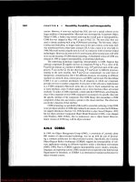
oxygen is 3 mL per liter of blood or 4 mg per liter of blood. Figure 10 presents the variation of
H(T) for various dissolved gases in liquid water.
E. DEVIATIONS FROM RAOULT’S LAW
Consider two species k and j that form a binary mixture. The attraction force between
similar molecules of species k is denoted as F
kk
and between dissimilar molecules as F
kj
. The
following scenarios ensue: (1) F
kj

= F
kk
so that the ideal solution model and Raoult’s Law ap-
ply, e.g., toluene–benzene mixtures and mixtures of adjacent homologous series; (2) F
kj
> F
kk
implying a nonideal solution in which contraction occurs upon mixing, e.g., acetone–water
mixtures and other examples of hydrogen bonding; and (3) F
kj
< F
kk
, which corresponds to a
nonideal solution in which the volume expands upon mixing, e.g., ethanol–hexane and other
polar–non polar liquids. In case of the second scenario, since the intermolecular attraction
forces are stronger between k–j pairs than between k–k molecular pairs, the vapor pressure of
species k can be lower than that predicted using Raoult’s Law, which is referred to as a nega-
tive deviation from the Law. In case (3) the attraction forces are lower, and a larger amount of
vapor may be produced as compared with the Raoult’s Law prediction, i.e., both the second
and third scenarios suggest that we must involve activity coefficients, γ
k(
l
)
. It will now be
shown that
p
k
= γ
k(
l

)
X
k,
l

p
k
sat
. (43)
where γ
k(
l
)
=
ˆ
f
k(
l
)
(T,P)/
ˆ
f
k(
l
)
id
(T,P) =
ˆ
f
k(

l
)
(T,P)/(X
k(
l
)
f
k(
l
)
(T,P)).
1. Evaluation of the Activity Coefficient
We have previously employed the ideal solution model to predict the vapor pressure
of a component k in an ideal solution. If the measured component vapor pressure differs from
that prediction, then it is apparent that the ideal solution model is not valid. We can determine
the activity coefficient (that represents the degree of non-ideality from the measured vapor
pressure data) as follows.
γ
k
=
ˆ
f
k
/
ˆ
f
k,id
=
ˆ
f

k
/X
k
f
k
(T,P). (44)
At phase equilibrium,
ˆ
f
k(g)
= γ
k(g)
X
k
f
k(g)
(T,P) =
ˆ
f
k(
l
)
and (45)
γ
k(g)
X
k
f
k(g)
(T,P)=

ˆ
f
k(
l
)
= γ
k (
l
)
X
k,
l
f
k(
l
)
(T,P). (46)
Since the vapor is assume to be an ideal gas mixture γ
k(g)
=1, and
f
k(g)(
T,P) = P. Therefore,
p
k
= γ
k(
l
)
X

k,
l
f
k(
l
)(
T,P), where (47)
f
k,
l
(T,P) = f
k(
l
)
(T,P
sat
) POY ≈ f
k(
l
)
(T,P
sat
) = P
sat
, i.e.,
p
k
= γ
k(
l

)
X
k,
l
f
k(
l
)(
T,P) = γ
k(
l
)
X
k,
l
P
sat
= γ
k(
l
)
p
k,Raoult
. (48)
Thus, γ
k(
l
)
is a measure of the deviation from Raoult’s law. With respect to the measured vapor
pressure at a specified value of X

k
, namely,
γ
k(
l
)
= p
k
/(X
k,
l
p
k
sat
), or γ
k,
l
= p
k
/p
k,Raoult
. (49)
Figure 10: Henry’s constant H(T) for the solubility of gases in water. (From S. S. Zum-
dahl, Chemistry, DC Heath and Company, Lexington, Mass, 1986. With permission.)
Recall that the γ
k
’s for any phase are related to (
g
E
/(

R
T)) (see Eqs. (114) to (117), Chapter 8).
If,
X
1(
l
)
X
2(
l
)

R
T/
g
E
= B´ + C´ (X
1(
l
)
- X
2(
l
)
), (50)
then we obtain the Van Laar Equations:
ln γ
1
= A(T) X
2(

l
)
2
/((A(T)/B(T)) X
1(
l
)
+ X
2(
l
)
)
2
, ln γ
2
= B(T) X
1(
l
)
2
/((X
1(
l
)

+ (B(T)/A(T)) X
2(
l
)
)

2
, where (51)
A (T) = 1/(B´- C´), and (52)
B(T) = 1/(B´ + C´). (53)
The constants A and B are generally weak functions of temperature, and for the bi-
nary mixture, one can solve for A and B as
A = ln γ
1(
l
)
(1+ (X
2(
l
)
ln γ
2(
l
)
)/(X
1(
l
)
ln γ
1(
l
)
))
2
, (54)
B= ln γ

2(
l
)
(1+ (X
1(
l
)
ln γ
1(
l
)
)/(X
2(
l
)
ln γ
2(
l
)
))
2
. (55)
At the azeotropic condition, at which X
k(
l
)
= X
k
, Eq. (47 ) assumes the form
p

k
= X
k(
l
)
P = γ
k(
l
)
X
k(
l
)

p
k
sat
. (56)
Thus,
γ
k(
l
)(
X
k,azeotropic
)= P/
p
k
sat
(T). (57)

The Wilson equation for activity coefficient has the form
ln γ
1(
l
)
= AX
2,
l
2
/((A/B) X
1(
l
)
+X
2(
l
)
)
2
, ln γ
2
(58)
= B X
1(
l
)

2
/(X
1(

l
)
+(B/A)X
2(
l
)
)
2
, (59)
ln γ
2(
l
)
= – ln(X
2(
l
)
+ X
1(
l
)
A
21
)+ X
1(
l
)(
A
12
/(X

1(
l
)
+ X
2(
l
)
A
12
)
– A
21
/(X
2(
l
)
+ X
1(
l
)
A
21
)).
As X
1(
l
)
→ 0,
ln γ
1(

l
)
= – ln A
12
+ 1 – A
21
,and ln γ
2(
l
)
= – ln A
21
+ 1– A
12
, where (60)
A
ij
= (v
j
/v
i
) exp (– a
ij
/R T),
and v
j
denotes the molal volume of species j, and a
ij
is a known constant that is independent of
composition and temperature, where a

ij
≈ a
ji
.
F. SUMMARY
This chapter summarizes relations for obtaining saturation properties for miscible and
immiscible mixtures. Using the phase equilibrium criteria of equal fugacities of any given
component in all phases, the composition in any phase can be determined at specified values of
T and P. Relations for dew point, bubble point, vapor/liquid composition, solubilities, etc., are
obtained. The methodology is extended to nonideal solutions.
G. APPENDIX
1. Phase Rule for Single Component
a. Single Phase
Both pressure and temperature can be varied independently for a single phase for a single
component. The system is bivariant with two degrees of freedom, i.e., F = 2.
b. Two Phases
If water is maintained at 180ºC with the condition that two phases must coexist, the pres-
sure P must be held at 1 MPa. Likewise, at 170ºC, P = 0.8 Mpa. Therefore, only one of the
two properties (P,T) is an independent variable in a two phase system. This system is
monovariant with a single degree of freedom.
c. Three Phases
The three phases of water coexist only at T = 0.01ºC and P = 0.006 bar. It is not pos-
sibly to vary either T or P if the three phase condition is desired. This system is invariant with
a zero degree of freedom.
d. Theory
We have seen that the phase rule
F = 3–π (Α)
applies, where π denotes the number of phases. At phase equilibrium between three phases,
say, the α, β, and γ phases,
µ

α
(P,T) = µ
β
(P,T) = µ
γ
(P,T). (Β)
Eqs. (B) represent two equations µ
α
=µ
β
and µ
β
= µ
γ
and, since there are two unknowns P and
T, the solutions are uniquely fixed so that F = 0.
2. General Phase Rule for Multicomponent Fluids
In a K component system,
Σ
K
X
k
= 1. (Β)
In this case, the number of variables specifying the chemical potential of each component in
each phase is ((K–1) +2). Thus for any phase j
µ
kj j j K j
XX X PT
() () () ()
(, ,, ,,)

12 1
K
−
, j = 1,2, …, π, and k = 1,2, …, K–1. (C)
The mole fractions of any component in the different phases are, in general, different.
From the phase equilibrium condition for any species k
µ
kK
XXPT
() () ()
(,, ,,)
111 11
K
−
=
µ
kK
XXPT
() () ()
(,, ,,)
212 12
K
−
=…=
µ
ππ πKK
XXPT
() () ()
(,, ,,)
11

K
−
, (D)
which represents a set of (π–1) equations. Overall, there are (π–1)K equations available that
relate the composition variables
1
1
k
1
2
K-1 2 K-1
X , X
X

X
X
X
(, ),(,, ),,(,, )
()
()
()
()
()
−1
1
1 π
π
and the
two intensive variables P and T. The total number of variables then equals (π(K–1)+2). Since
these variables are related by (π–1)K equations, the number of degrees of freedom is

F = π (K–1) + 2 – (π–1)K = K – π + 2, (E)
which is known as Gibbs phase rule. The phase rule is usually applied to a system of K com-
ponents and π phases at specified values of P and T.
l. Example 12
steam.?
Solution
K = 1 (for a single component), π = 1 (for a single phase). Therefore, F = 2.
Remarks
For a mixture of liquid water and steam, K = 1, π = 2, and F = 1. It is a monovariant
system.
Likewise, for a mixture of ice, liquid water, and steam, F = 0.
m. Example 13
grees of freedom.
F = 2 + 2 – 1 = 3.
Solution
This is a trivariant system, e.g., we can independently assign the variables T, P, X
1
.
F = 2 + 2 –2 = 2
n. Example 14
namely, liquid and gaseous. Determine the number of degrees of freedom.
Solution
If the system is nonreacting,
F = 3 + 2 – 2 = 3
If the system is reacting according to the chemical reaction
H
2
SO
4
(l) + Ca(s) → H

2
(g) + CaSO
4
(s),
the chemical equilibrium condition requires that
ˆ
g
HSO
24
+
ˆ
g
Ca(s)
=
ˆ
g
H
2
+
ˆ
g
CaSO s
4
()
.
This restriction reduces the number of freedom by 1, and
F = 3 – 1 = 2.
If the number of equilibrium reactions are R (Chapter 12), the number of degrees of
freedom is modified to be
F = K +2 – π – R.

Generalizing for all work modes,
F = K + 1 + work modes – π – R
o. Example 15
rium with the liquids. What is the phase rule for this case?
Solution
F = K + 2 – π, where π = 3 (the two pure solid phases and the one liquid phase) and K
= 2, so that
F = 2 + 2 – 3 = 1.
3. Raoult’s Law for the Vapor Phase of a Real Gas
If a liquid mixture exists at a high pressure and low temperature, its vapor phase must
be treated as a real gas mixture, i.e.,
ˆ
f
k
1
(T,P,X
k,
l
) =
ˆ
f
k
g
(T,P,X
k
).
Applying an ideal solution and ideal mixture model,
Consider a binary mixture of species 1 and 2 in the liquid phase, which on cooling
forms two separate pure solids, one for each component. These solids are in equilib-
Consider a nonreacting system containing H

2
SO
4
(l), Ca(s), and H
2
(g) in two phases,
A single liquid phase is desired for a mixture of water and alcohol. Determine the de-
How many independent intensive variables are required to fix the state of superheated
X
k,
l
ˆ
f
k
1
(T,P) = X
k
ˆ
f
k
g
(T,P).
A species may exist as a gas at a specified temperature and pressure when alone (e.g., water at
110ºC, 100 kPa), but as a liquid in a liquid mixture with another higher boiling temperature
component. In that case,
ln (f
k
(T,P)/f
k
(T,P

sat
)) =
P
P
sat
∫
(v
k
/(RT)) dP.
If the hypothetical state is a liquid, then
ln (
f
k
l
(T,P)/
f
k
l
(T,P
sat
)) =
P
P
sat
∫
(
v
k
l
/(RT)) dP.

Since
v
k
l
is a small quantity,
f
k
l
(T,P) =
f
k
l
(T,P
sat
).
Similarly, for the gaseous state,
ln (
f
k
g
(T,P)/
f
k
g
(T,P
sat
)) =
P
P
sat

∫
(
v
k
g
/(RT)) dP.
Since ∫Z d(ln P) = ∫(v/RT) dP = (Pv/RT) – ∫((P/RT) dv)), applying the RK equation either
for the liquid or gaseous state, we can apply the expression
∫(v/RT)dP = (v/(v–b) – a/(RT
3/2
(v+b))) – ln (v–b) + (a/(RT
3/2
b)) ln (v/(v+b)).
Chapter 10
10. STABILITY
A. INTRODUCTION
The entropy maximum and energy minimum principles will be used to derive the sta-
bility criteria for a fluid that exists at a specified state. This will allow us to stipulate the phase
change conditions (e.g., evaporation and condensation) for single and multicomponent fluids.
Applications will also be presented.
The various equilibrium states of mechanical systems are illustrated in Figure 1.
States B, C, D, and F represent mechanical equilibrium positions (or states) while A is a non-
equilibrium position (and, hence, not a state). The equilibrium states B, C, and D can be classi-
fied according to their stability behavior by conducting perturbation tests as follows. An equi-
librium state is disturbed from its initial state by a small amplitude perturbation that changes
the potential energy. If a ball returns to its original state, that state is stable. The mechanical
stability behavior can be characterized by several states. Figure 1 illustrates a stable state (e.g.,
state D corresponding to a minimum potential energy), an unstable state (e.g., state C that has a
locally maximum potential energy), a metastable state (e.g., state B that can be perturbed to
potential energy levels, but which have finite constraints that require a relatively large distur-

bance to overcome), and a neutrally stable state (e.g., state F that has an invariant potential
energy). A disturbance at state C that is a point of maximum potential energy will cause a ball
placed there to move to either of positions B or D that are more stable. Therefore, stability can
also be defined with respect to a disturbance from an equilibrium state. State C is unstable
since any disturbance causes the ball to move towards either State B or State D which are the
next equilibrium states in the immediate vicinity of State C. Thus State C is impossible to
achieve in a practical system. The state C is equivalent to a nickel standing on its edge in the
absence of a disturbance. A slight disturbance, however, can cause the nickel to fall flat on the
surface.
If the ball at B is disturbed (e.g., by a potential energy disturbance) by a finite
amount, then ball may move to a more stable state D which has the lowest energy of all states
illustrated in Figure 1. The rate at which the ball returns to its original state depends upon the
friction between the ball and surface. If the potential energy constraint mgZ

is removed, the
ball will eventually roll to position D. State D is the most stable equilibrium state, state C is
unstable and state B is
a metastable equilib-
rium state. As long as
constraints exist in the
mechanical system of
Figure 1 and the distur-
bances are minor, a
metastable system is
also a stable system.
During a me-
chanical disturbance
test the potential energy
is changed from its
initial level in order to

determine if its value
increases or decreases.
In that context, state C
is unstable since d(PE)
< 0, but state D is sta-
Z
c
Z
D
Z
B
Figure 1: Illustration of various mechanical states.
ble since d(PE) > 0 with disturbance. A distur-
bance to State D (cf. Figure 1) creates a non-
equilibrium situation (i.e., towards higher poten-
tial energy locations as d(PE) > 0), which induces
the ball to roll back. This process brings the ball
back to state D and decreases the potential energy
by converting it into kinetic energy. Any pertur-
bation of a stable equilibrium state causes a proc-
ess that tends to attenuate the disturbance. This is
also known as the Le Chatelier principle and is a
consequence of the Second Law.
Consider a thermodynamic system with
water as working fluid (cf. Figure 2). The path
AFGH is a 40 bar isobar and all states along
AFGH are stable analogous to the state D in
Figure 1. However, it is possible to reach superheated liquid states along FM (except the point
M) which are analogous to state B in Figure 1. Similarly, if vapor at state H is cooled. Simi-
larly if vapor at state G is cooled, it can be cooled to a vapor state to along GN in the form of

subcooled vapor. Again, states along path GN (except at point N) are analogous to state B.
Likewise, the states along the path MN are analogous to state C in Figure 1. In a manner simi-
lar to mechanical stability tests, we can test the stability of fluids along the paths HGN or AFM
by perturbing the system (e.g., by disturbing the volume from a value V to V + dV) and deter-
mining if the system returns to its original state. The rate of return to the stable equilibrium
state for any fluid depends upon transport rate processes, e.g., heat and mass transfer, which is
beyond the scope of classical thermodynamics.
If one strikes a match in air, the match simply burns and extinguishes. This implies
that the constituents of air do not react at a significant rate. On the other hand, if a match is
ignited in air in the presence of a significant amount of gasoline vapors (i.e., if the reactive
mixture is in metastable equilibrium), small temperature disturbances can ignite the mixture. In
general, if a disturbance decreases the entropy of an isolated system at specified values of U, V
and m, then the system must initially have been at a stable equilibrium state (SES). Note that
what is known as “equilibrium” in the context of classical thermodynamics yields only an av-
erage state (e.g., an average system temperature or pressure) while any real system is inces-
santly dynamic at its microscopic level. Thus, a system should be stable with inherent micro-
scopic and small natural disturbances.
B. STABILITY CRITERIA
1. Isolated System
An example of an isolated system is one constrained by rigid adiabatic and impermeable
walls, i.e., with specified values of U, V, and m. An isolated system is at equilibrium when its
entropy reaches a maximum value so that δS = 0. At this state, if the system is perturbed such
that the values of U, V, and m of the system are unchanged (e.g., by increasing the temperature
or internal energy by an infinitesimal amount), the perturbations are dampened since the sys-
tem is stable. The perturbations at fixed values of U, V, and m actually decrease the entropy,
i.e., δS < 0 at stable equilibrium. (e.g., consider adiabatic chemical reactions, Chapter 11).
a. Single Component
In Chapters 6 and 7 we employed the real gas state equation and evaluated various
thermodynamic properties. Let us consider the compression of water in the context of the RK
equation of state is, say, at 593 K and 1 bar. The volume of water decreases (or its intermo-

lecular spacing decreases) and the pressure first increases, then decreases with a further de-
crease in the volume, and again increases. Since the intermolecular spacing continuously de-
creases, stability analysis can help determine the state at which the fluid becomes a liquid.
T
v
Figure 2: Thermodynamic states of wa-
ter.
First, let us consider an isolated system with specified values of U, V and m and ex-
press S = S(U, V, m). From Chapter 7,
s = s (T,v) and u = u(T,v), i.e., s = s(u,v), (1)
which is the entropy fundamental equation.
a. Example 1
28 kJ kmole
–1
. Select the reference condition such that
s = c
v0
ln (u/c
v0
+ a/(v c
v0
)) + R ln (v–b).
Plot the entropy vs. volume for an internal energy value of 7000 kJ kmole
–1
.
Solution
Since
du = c
v
dT + (T (∂P/∂T)

v
– P) dv,
du
T
= (T(∂P/∂T)
v
– P) dv. (A)
Using
P = RT/(v–b) – a/v
2
(B)
in Eq. (A),
du
T
= T(R/(v–b)) – (RT/(v–b) – a/v
2
) = (a/v
2
) dv
Integrating at constant temperature,
u(T,v) = –a/v + f(T). (C)
In case a = 0,
u
0
(T) = f(T). (D)
Eliminating f(T) between Eqs. (C) and (D),
u(T,v) = u
0
(T) – a/v. (E)
Assuming constant (ideal gas) specific heats and u = u

ref,0
at T = T
ref
,
u
0
(T) – u
ref,0
= c
v0
(T – T
ref
), (F)
Eq. (E) assumes the form
u = c
v0
(T–T
ref
) + u
ref,0
– a/v, i.e., (G)
T = ((u–u
ref,0
) + a/v)/c
v0
+ T
ref
. (H)
Similarly, we can integrate the expression
ds = c

v
dT/T + ∂P/∂T dv
at constant temperature to obtain the relation
s(T,v) = s
0
(T,v) – R ln (v/(v–b)). (I)
Using the ideal gas relation for s
0
(T,v),
s
0
(T,v) – s
ref,0
(T
Ref
,v
ref
) = c
v0
ln (T/T
Ref
) + R ln (v/v
ref
),
Consider the Van der Waals equation of state. Obtain an expression for s = s(u,v) for
water assuming the specific heat to be constant and equal to the ideal gas value c
v0
=
s(T,v) = c
v0

ln (T/T
Ref
) + R ln (v/v
ref
) + s
ref,0
(T,v
ref
)– R ln (v/(v–b)). (J)
Further, using Eqs. (H) and (J) to eliminate the temperature,
s =c
v0
ln((u–u
ref,0
)/(c
v0
T
ref
)+(a/(vc
v0
T
ref
) + 1)+R ln((v–b)/v
ref
+s
ref,0
(T
Ref
,v
ref

). (K)
Setting ,
s
ref,0
(T
ref
,v
ref
) =c
v0
ln(c
v0
T
ref
) + R ln v
ref
, u
ref,0
= c
v0
T
ref
we obtain the expression
s = c
v0
ln (u + a/v) + R ln ((v–b)). (L)
For ideal gases, a = b =0, and Eq. (K) leads to the relation
s
0
= c

v0
ln (u/(c
v0
T
Ref
)) + R ln (v/v
Ref
) (M)
This expression leads to a plot of s vs. both u and v for a real or ideal gas.
Using the values
¯a
= 5.3 bar m
6
kmole
–2
,
¯b
= 0.0305 m
3
kmole
–1
,
u
= 7000 kJ
kmole
–1
, T
ref
= 1 K,
v

ref
= 1 m
3
kmole
–1
,
c
v0
= 28 kJ kmole
–1
K
–1
,
u
ref,0
=
c
v0
T
ref
= 28
kJ kmole
–1
in Eq. (K), a plot of s vs. v at u = 7500 kJ kmole
–1
is presented in Figure 3.
Remarks
The relation s =s (u,v) is the entropy fundamental equation. It is somewhat more diffi-
cult to manipulate the RK equation and obtain an explicit expression for s = s(u,v)
using Eq. (L).

b. Example 2
internal energy. What is the entropy change during the process? (Use Figure 3.)
Solution
The fluid molecules are distributed uniformly in the tank and initially,
v
1
=
v
2
=
v
=
0.4÷4 = 0.1 m
3
kmole
–1
. Using Figure 3 or Eq. (K) of Example 1, we note that

¯s
=
149.83 kJ kmole
–1
. The state is represented by point D in the figure, and the extensive
146
146.5
147
147.5
148
148.5
149

149.5
150
150.5
151
0.04 0.05 0.06 0.07 0.08 0.09 0.1 0.11 0.12 0.13 0.14 0.15 0.16 0.17 0.18 0.19 0.2
v, m
3
/ kmol
e
s, kJ/ kmole K
L
C
M
K
B
H
A
N
D
E
L
iqui
d
G
as
y
Figure 3: Variation in the entropy vs. volume for water
modeled as a VW fluid at u = 7500 kJ kmole
–1
.

Consider a rigid and insulated 0.4 m
3
volume tank filled with 4 kmole (24×10
26
mole-
cules) of water, and an internal energy of 7500 kJ kmole
–1
. Divide the tank into two
equal 0.2 m
3
parts. Assume that water follows the VW state equation. What is the en-
tropy of each section? Assume that section 1 is slightly compressed to 0.14 m
3
while
the section 2 is expanded to 0.26 m
3
, but maintaining the same total volume and total
entropy of each section is initially
S
D
= (S
1
= N
1

¯s
1
) = (S
2
= N

2

¯s
2
) = 2×149.83 =299.7 kJ. (A)
The total entropy of the tank is S = 2S
D
= 299.7 + 299.7 = 599.4 kJ. After the pertur-
bation,
v
1
= 0.14÷2 = 0.07 m
3
kmole
–1
, u
1
= 7500 kJ kmole
–1
, and
v
2
= 0. 26÷2 = 0.13 m
3
kmole
–1
, u
2
= 7500 kJ kmole
–1

.
The corresponding states are represented by points M and N in Figure 3, i.e.,
S
M
= S
1
= N
1

¯s
1
= 2×149.8 = 299.6 kJ, and
S
N
= S
2
= N
2

¯s
2
= 2×149.9 = 299.9 kJ.
The total entropy after the disturbance
S = S
1
+ S
2
= S
M
+ S

N
= 599.5 kJ.
Remarks
We note that the entropy (at specified values of U, V and m) increases after the dis-
turbance, i.e., S
M
+ S
N
> 2 S
D
. Therefore, the initial state is unstable and changes in
the direction of increasing entropy. At states B and E disturbances no longer cause a
further increase in the entropy.
2. Mathematical Criterion for Stability
a. Perturbation of Volume
i. Geometrical Criterion
Consider the state B illustrated in Figure 3 which undergoes a small disturbance ∆V at
a specified value of U. Due to the disturbance, Section 1 of the system in Example 2 reaches
state L while Section 2 reaches state M (Figure 3) . With respect to stability
δS = δS
1
+ δS
2
< 0, i.e., (2)
δS = (S
L
(U,V–∆V,N) – S
B
(U,V,N)) + (S
M

(U,V+∆V,N) – S
B
(U,V,N)) < 0.
Since
δS = S
L
(U,V–∆V,N) + S
M
(U,V–∆V,N) – 2S
B
(U,V,N) < 0, i.e.,
(S
L
(U,V–∆V,N) + S
M
(U,V–∆V,N))/2 < (S
B
(U,V,N). (3)
The entropy after a disturbance decreases in order that the initial state of the system is stable.
In the context of Figure 3, the ordinate of the midpoint C of the chord LCM that connects the
points L and M is represented by the LHS of Eq. (3) while the RHS represents the ordinate of
the point B. Therefore, the chord LCM must lie below the curve LBM for the system to be
stable. The curve LKBHM satisfying the criteria given by Eq. (3), is a concave curve with re-
spect to the chord LCM. On the other hand, the midpoint of the chord MAN lies above the
convex curve MDN, thereby violating this stability criterion. We find that for a system to be
stable the fundamental relation for S = S (U, V, N) one must satisfy the concave condition,
which is established by Eq. (3).
ii. Differential Criterion
The discussion so far pertains to disturbances, which are of large magnitude ∆V. Con-
sider a disturbance is in the neighborhood of state B (cf. Figure 3) that extends from state K at

(U, V–∆V, N) to state H at (U, V + ∆V, N). In that case
(δS = (S
K
(U,V–∆V,N)–S
B
(U,V,N)) + (S
H
(U,V+∆V,N)–S
B
(U,V,N))) < 0, (4)
where δS denotes the entropy change due to the disturbance. The entropy should decrease fol-
lowing disturbance at the stable points A, B and E illustrated in Figure 4. Expanding S
K
and
S
H
in a Taylor series
S
K
(U, V–∆V, N) = S
B
+ (∂S/∂V)
B
(–dV) + (1/2!)(∂
2
S/∂V
2
)
B
(–dV)

2
+ , and
S
H
(U, V+dV, N) = S
B
+ (∂S/∂V)
B
(dV) + (1/2!) (∂
2
S/∂V
2
)
B
(dV
2
) + , i.e.,
δS = S
B
+ (∂S/∂V)
B
(–dV) + (1/2!)(∂
2
S/∂V
2
)
B
(–dV)
2
+ +

S
B
+ (∂S/∂V)
B
(dV) + (1/2!)(∂
2
S/∂V
2
)
B
(dV)
2
+ – 2 S
B
(U, V, N) < 0.
We will represent the contribution to the disturbance by the first derivatives in the form
dS
B
= (∂S/∂V)
B
(–dV) + ((∂S/∂V)
B
(dV) = 0,
and by the higher–order derivatives as
d
2
S
B
= (1/2!)(∂
2

S/∂V
2
)
B
(–dV)
2
+ (1/2!)(∂
2
S/∂V
2
)
B
(dV)
2
+ ….
So that Eq. (4) assumes the form
(δS = (dS)
B
+ (d
2
S)
B
) < 0.
Since (dS)
B
= 0,
(δS = (d
2
S)
B

= (∂
2
S/∂V
2
)
B
(dV)
2
) < 0.
Omitting the subscript B, the general criteria for stability at any given state that
(dS) = 0, and (d
2
S) < 0, (5)
which are the same as the conditions for entropy being maximized at specified values of U, V
and N (stable points A, B and E and unstable point D in Figure 4). Since (dV)
2
> 0, the rela-
tion
(∂
2
S/∂V
2
) < 0 (6)
must be satisfied in the neighborhood of an equilibrium state for it to be stable. If case the sec-
ond derivatives are zero, the third derivatives in Taylor series are included to obtain the stabil-
ity condition d
3
S < 0, and so on.
c. Example 3
s

vv
= ∂
2
s/∂v
2
< 0 at all volumes.
Solution
We will employ the relations
Tds – P dv = du and ds = du/T + P/T dv.
At constant internal energy
Assume that water follows the ideal gas state equation and show that for a unit mass,
(∂s/∂v)
u
= P/T, and
since for ideal gases, P/T = R/v,
s
v
= (∂s/∂v)
u
= R/v = f(v) alone, and
s
vv
=(∂
2
s/∂v
2
)
u
= –R/v
2

< 0
Remark
This illustrates that ideal gases are stable at all states.
Figure 5 contains plots of

¯s
vs.

¯v
at various values of

¯u
. At very high values of
¯u
(e.g., at temperatures larger than the critical temperature), the fluid is stable for any vol-
ume, i.e., there is no increase in entropy in the presence of a disturbance at any state. For a
solid there are certain regimes in which stability criteria are not satisfied and disturbances re-
sult in phase transitions. e.g., in case of water from ice–phase I, to ice–phase II.
Since, in our illustrations, U, V and N (or m) were specified during a disturbance, the
D
U(D) plane
d
2
S>0
d
2
S < 0
d
2
S < 0

Disturbed
Volume
D
Figure 4: Illustration of the entropy perturbation following a disturbance in the vol-
ume of sections 1 and 2 of a rigid container.
relation
δW
opt
= – dU + T
0
δS,
with disturbance at a stable state yields
δW
opt
= T
0
δS < 0. (7)
If the system is initially unstable (cf. State D in Figure 1), then δW
opt
> 0, i.e., the system could
have performed work during the entropy increase in the isolated system.
b. Perturbation of Energy
Repeating the procedure outlined in the previous section, but with the disturbance pa-
rameter in terms of U, it is again possible to show that for stability
S
UU
= (∂
2
S/∂U
2

) < 0, (8)
which is identical to the “concavity condition” described previously.
Consider the plot of entropy vs. internal energy at specified values of N (or m) illus-
trated by the curve ABCDEFGH in Figure 6 for a fluid following a real gas equation of state.
At some equilibrium states d
2
S >0 (i.e., these states are unstable) and at others, d
2
S < 0 (stable
states). In the context of Figure 6 consider the fluid at state B at which the curve ABC is con-
cave with respect to U. Here, the stability criterion is satisfied. On the other hand, curve DEF
is convex, the criterion is violated.
A plot of (∂S/∂U)
V
= 1/T vs. U is presented in Figure 6b and that of T vs. U is illus-
trated in Figure 6c. It is apparent that for certain ranges of U (U
D
to U
F
), T decreases with in-
creasing U. Mathematically, the stability condition ∂
2
S/∂U
2
< 0 is equivalent to the condition
(∂/∂U)(∂S/∂U) < 0, i.e., ∂/∂U(1/T) < 0 or –1/T
2
(∂T/∂U) < 0. (9)
In the context of Eq. (9), since (∂U/∂T) = mc
v

, then mc
v
> 0, and at a specified value of either
m or N,
c
v
> 0 (10)
145
147
149
151
153
155
157
159
0.02 0.07 0.12 0.17 0.22 0.27
v, m
3
/ kmole
s, kJ/ kmole K
u
= 7500 kJ/kmole
1
0000
9
500
9
000
8
500

8
000
10000
Figure 5: Variation of s vs. v in case of water according to the VW state equation.
for a state to be stable. In Figure 6c, c
v
has positive values along the branch ABCD but nega-
tive values along DEF, which violates the thermal stability criterion provided by Eq. (10). The
negative c
v
values imply that temperature decreases when energy is added and increase when
heat is removed. Consider water at 25ºC and 1 bar in an insulated cup and assume that it has
negative specific heat. Divide the water into two equal sections A and B. We now discuss the
meaning of thermal stability. If the water is thermally disturbed with a small amount of heat
transfer δQ from A to B, then A will continue to become warmer than B (due to larger storage
of energy as intermolecular potential energy and less as vibrational energy) with the distur-
bance. The entropy generation is still positive for the adiabatic cup since δσ = δQ (1/T
A
–1//T
B
) > 0 as T
A
> T
B
. It still satisfies Second Law with entropy generation indicating that the
initial state is thermally unstable.
The specific heat c
v
> c
vo

for fluids following the RK equation, where c
vo
> 0. This
implies that a curve representing variations in S vs. U must be concave (i.e., it must have a
decreasing radius of curvature) with respect
to U at a specified value of V. In other
words, thermal stability is always satisfied
for satisfying most of the real gas state
equations. Read Example 17 for instances
when this may be violated.
d. Example 4
(s
uu
= ∂
2
s/∂u
2
) < 0 at all volumes.
Solution
Consider the relation T ds – P dv =
du. At fixed volume
∂s/∂u = 1/T.
Differentiating this expression,
∂
2
s/∂u
2
= –1/T
2
(∂T/∂u)

v
.
Since
(∂u/∂T)
v
= c
v
,
(∂
2
s/∂u
2
= –1/(c
v
T
2
)) < 0.
Remarks
For a real gas,
(∂c
v
/∂v)
T
= T(∂P/∂T
2
)
v
,
i.e., for a VW gas
(∂c

v
/∂v)
T
= 0,
which implies that c
v
= f(T) = c
v0
(T) >0
A VW gas is thermally stable at all points.
c. Perturbation with Energy and Volume
The discussion so far has pertained to disturbance in the internal energy at specified
volume or in the volume at specified values of U. If the volume and energy are both perturbed,
the following conditions must be satisfied, i.e.,
δS = S(U+dU, V+dV, N) + S(U–dU, V–dV, N) – 2 S(U, V, N) < 0, i.e.,
S(U+dU, V+dV, N) + S(U–dU, V–dV, N) < 2 S(U, V, N).
Expanding this expression in a Taylor series, and retaining terms up to the second derivative,
G
H
H
F
F
G
Figure 6: Qualitative illustration of the varia-
tion of a) entropy, b) ∂S/∂U=1/T and c) tem-
perature with respect to the internal energy.
Consider a VW gas and show that
δS = (∂S/∂U dU + ∂S/∂V dV + (∂/∂U + ∂/∂V)
2
S) +

(–∂S/∂U dU – ∂S/∂VdV +(∂/∂U + ∂/∂V)
2
S) < 0
Since,
dS = (∂S/∂U dU + ∂S/∂V (–dU)) + (∂S/∂V dV + ∂S/∂V (–dV)) = 0, then
(∂/∂U + ∂/∂V)
2
S < 0
Expanding this relation, we obtain the expression,
(d
2
S = ∂
2
S/∂U
2
dU
2
+ 2(∂
2
S/∂U∂V)dU dV + ∂
2
S/∂V
2
dV
2
) < 0, i.e.,
(d
2
S = S
UU

dU
2
+ 2 S
UV
dU dV + S
VV
dV
2
) < 0. (11)
Multiplying Eq. (11) by S
UU
, since S
UU
< 0, Eq. (11) assumes the form
(d
2
S = S
UU
2
dU
2
+ 2 S
UU
S
UV
dU dV + S
UU
S
VV
dV

2
) > 0, i.e., (12)
(S
UU
dU + S
UV
dV)
2
+ (S
UU
S
VV
– S
UV
2
) dV
2
> 0 (13)
Now, (S
UU
dU + S
UV
dV)
2
> 0, and since dV
2
> 0, it is apparent from the perspective of stability
that
(S
UU

S
VV
– S
UV
2
) > 0, (14)
which is the stability condition in the presence of volumetric and energetic fluctuations within
a system. The stability criterion at a given state can be summarized as
D
1,U
= S
UU
= ∂
2
S/∂U
2
< 0, and D
1,V
= S
VV
= ∂
2
S/∂V
2
< 0, (15)
In determinant form, the stability criterion is
D
SS
SS
UU UV

VU VV
2
0=>
(16)
where D
2
is determinant of second order. If D
1,U
< 0, and D
2
> 0, then D
1,V
< 0. It is noted that
since ∂s/∂u = 1/T, then s
vu
=(∂
2
s/∂v ∂u)= –(∂T/∂v)
u
/T
2
.
e. Example 5
For an ideal gas show that Eq. (16) applies for all volumes.
Solution
From Example 1 we note that s
vv
< 0, and from Example 2 that s
uu
< 0.

Since ∂s/∂u = 1/T, then s
vu
= ∂
2
s/∂v ∂u = –(∂T/∂v)
u
/T
2
.
If the energy of an ideal gas is specified, its temperature cannot change with respect to
changes in the volume. For this reason (∂T/∂v)
u
= 0. Therefore,
s
vu
= 0, and
using Eq. (16)
s
uu
s
uu –
s
vu
s
vu
> 0,
which satisfies the stability criterion.
f. Example 6
Apply the RK equation of state