ADVANCED THERMODYNAMICS ENGINEERING phần 6 ppt
Bạn đang xem bản rút gọn của tài liệu. Xem và tải ngay bản đầy đủ của tài liệu tại đây (1.36 MB, 80 trang )
jj. Example 36
temperature?
Solution
µ
JT
= (∆h/c
p
)/∆P = ∆T/∆P = (T
e
–203)/(40 – 60) = 0.31 K bar
–1
. Therefore, T
e
=
–73.2ºC.
a. Evaluation of
µ
JT
Recall that
dh = c
p
dT + (v – T(∂v/∂T)
P
)dP.
Since dh ≈ 0 during throttling, we obtain the relation
µ
JT
= (dT/dP)
h
= –(v – T(∂v/∂T)
P
)/c
P
= (T
2
/c
P
) ∂(v/T)/∂T, or (156)
µ
JT
= (dT/dP)
h
= –(1 – Tβ
P
)/(c
P
/v). (157)
b. Remarks
For ideal gases, v = RT/P so that T(∂v/∂T) = v and, hence, µ
JT
= 0. There is no tem-
perature change due to throttling for ideal gases.
For incompressible fluids ∂v/∂T = β
P
= 0, and µ
JT
= –v/c
P
has a negative value. There-
fore, liquids generally heat up upon throttling.
If v < T(∂v/∂T)
P
or T β
P
< 1, µ
JT
> 0, and vice versa.
At the inversion point, µ
JT
= 0. Inversion occurs when T
inv
β
P
= (T/v)(∂v/∂T)
P
= 1. For
a real gas Pv = ZRT, i.e., ∂v/∂T = ZR/P + (RT/P)∂Z/∂T. If (T/v)(∂v/∂T)
P
= 1, this im-
plies that ZRT/Pv + (RT
2
/Pv)∂Z/∂T = 1, or (∂Z/∂T)
P
= 0.
For cooling to occur, the inlet pressure must be lower than the inversion pressure.
Cooling of a gas can also be accomplished using isentropic expansion. We define µ
s
=
(∂T/∂P)
s
that is related to the temperature decrease due to the work delivered during
an isentropic process. Recall that
ds = c
p
dT/T – (∂v/∂T)
P
dP.
For an isentropic process, ds = 0, and
µ
s
= T(∂v/∂T)
P
/c
P
= Tvβ
P
/c
P
. (158)
Dividing Eq.(157) by Eq.(158),
µ
JT
/µ
s
= 1 – (1/(Tβ
P
)) (159)
Equation (159) provides a relation to indicate relative degree of heating of the isen-
tropic to isenthalpic throttling process.
For substances that expand upon heating β
P
> 0 and, hence, µ
s
> 0. If β
P
T > 1, then
µ
JT
< µ
s
, i.e., the isentropic expansion results in greater cooling than isenthalpic ex-
pansion for the same pressure ratio.
The values of T
inv
, β
P
, β
T
, and P
sat
can be directly obtained from the state equations,
while µ
JT
, h, u, c
v
, and other such properties depend both on the equations of state and
The experimentally determined value of µ
JT
for N
2
is 0.31 K bar
–1
at–70°C and 5
MPa. If the gas is throttled from 6 MPa and –67ºC to 4 MPa, what is the final exit
the ideal gas properties. Therefore, the accuracy of the state equations of state can be
directly inferred by comparing the predicted values of T
inv
, β
P
, β
T
, and P
sat
with ex-
perimental data.
The entropy change during an adiabatic throttling process equals the entropy gener-
ated. Therefore, its value must be positive, since throttling is an inherently irreversible
process. We can determine ds by using the following relation:
dh = T ds + v dP.
Since dh = 0,
K
L
A
B
µµ
µµ
JT
= 0
µµ
µµ
JT
<0
µµ
µµ
JT
> 0
Inversion
Curve
(b)
P
i
P
e
P
A
P
B
(a)
Exit
Figure 20: (a) Illustration of a throttling process. (b) The
variation of temperature with respect to pressure during throt-
tling.
(∂s/∂P)
h
= – (v/T). (160)
During throttling, dP
h
< 0 and v/T > 0; hence Eq.(160) dictates that ds
h
>0. From second
law for fixed mass adiabatic system, ds
h
(= δσ) =-(v/T) dP
h
> 0.
kk. Example 37
Obtain an expression for µ
JT
for a VW gas in terms of v and T.
Solution
The Joule Thomson coefficient
µ
JT
= – (∂h/∂p)
T
/c
p
, where (A)
(∂h/∂p)
T
= v – T (∂v/∂T)
p
. (B)
Using the VW equation of state
dP = R dT/(v – b) + (–RT/(v – b)
2
+ 2 a/v
3
)dv. (C)
Since dP = 0,
(dv/dT)
p
= (R/(v – b))/(RT/(v – b)
2
– 2 a/v
3
) (D)
Therefore,
µ
JT
= – (1/c
p
) (v – ((T R/(v–b))/(RT/(v–b)
2
– 2 a/v
3
))), i.e., (E)
µ
JT
= – (v/c
p
)(R T b v
2
– 2 a (v – b)
2
)/(RTv
3
– 2 a (v – b)
2
)). (F)
Remarks
For many liquids v ≈ b, i.e.,
µ
JT
≈ –v/c
p
for liquids.
Since µ
JT
< 0, incompressible liquids will heat up upon throttling.
In context of Eq.(F), if b « v, (v–b)
2
≈ v
2
. Consequently, using Eq.(F),
µ
JT
= –(v/c
p
) (RTbv
2
– 2 a v
2
)/(RTv
3
– 2 a v
2
)). (G)
Dividing the denominator and numerator by RTv
2
,
µ
JT
= – (v/c
p
)(b – 2a/RT)/(v –2a/RT) (H)
If v » (2a/RT), e.g., for high temperature vapors,
µ
JT
≈ ((2 a /RT)–b)/c
p
. (I)
At low temperatures, 2a/RT » b, and µ
JT
>0, i.e., cooling occurs upon throttling. At
higher temperatures, µ
JT
< 0 (i.e., the fluid is heated upon throttling).
In the limit T→∞ (when the fluid approaches ideal gas behavior), Eq. (F) implies that
µ
JT
= –b/c
p
, i.e., µ
JT
c
p
/v
c
´ = –b/v
c
´ = –1/8. This limiting value is based on the real gas
equation of state. However, for ideal gases, µ
JT
= 0, since b→0 for the ideal gas point
mass molecules. Recall that b equals the geometrical free volume available for mole-
cules to move around. The corresponding result using the RK equation is µ
JT
c
P
/v
c
´ ≈
–b/v
c
´≈ –0.08664.
2. Temperature Change During Throttling
Recall from Chapter 2 that the internal energy of unit mass of any fluid can be
changed by frictional process and by performing boundary deformation work (Pdv). For in-
compressible fluid, dv=0 and hence boundary deformation work is zero; thus "u" can change
only with a frictionless process (e.g., flow of liquids through pipes) where the mechanical part
of energy “vdP” is converted into internal energy using frictional processes. Thus a combi-
nation of both of the processes Pdv and vdP result in temperature change during the throttling
process.
a. Incompressible Fluid
Assume that an incompressible fluid is throttled from a higher to a lower pressure un-
der steady state conditions. Let us follow unit mass as it enters and exits the throttling device.
Since dv=0, there is no deformation work and hence u cannot change due to Pdv. However the
unit mass is pushed into the throttling device with a pump work of vP
i
, while the same mass is
pushed out with a pump work of vP
e
. Thus there must have been destruction of mechanical
energy from vp
i
to vP
e
which is converted into thermal energy (see Chapter 2) resulting in an
increase of u and hence an increase of T during throttling. The energy increases by an amount
du = –vdP ≈ –v(P
e
– P
i
). (Alternately dh =du+ pdv+ vdp = du +0+ vdp=0.) Also, recall that µ
JT
≈ – v/c
P
< 0. Further throttling is inherently irreversible process and hence entropy always in-
creases in adiabatic throttling process (e.g., increased T causes increased s).
b. Ideal Gas
Now consider a compressible ideal gas. Visualize the throttling process as a two step
procedure. First the specific volume is maintained as though fluid is incompressible and the
energy rises by the amount du = –vdP. This leads to gas heating. Now let the volume increase
during the second stage (i.e expansion to low pressure). The volume increase cannot change
the intermolecular potential energy, since the gas is ideal, but Pdv work is performed. This
leads to decrease in the internal energy. The total energy change is du = – vdP – Pdv = – d(Pv),
i.e., or du + d(Pv) = dh = 0. For ideal gases, dh = c
p
dT, and, hence, dT = 0. In this case, the
energy decrease by the Pdv deformation work equals the energy increase due to pumping (=-
vdP)
c. Real Gas
In a real gas the additional work required to overcome the intermolecular attraction
forces (or the increase in the molecular intermolecular potential energy, “ipe”) must be ac-
counted for. Then the temperature can decrease if increase in “ipe” is significant. Consider the
relation
dh = du + d(Pv) = du +P dv + v dP.
Since du = c
v
dT + (T (∂P/∂T)
v
– P) dv,
dh =c
v
dT + (T(∂P/∂T)
v
– P)dv + Pdv + vdP. (161)
The terms on the RHS of this equation, respectively, denote (1) the change in the temperature
due to change in the molecular translational, vibrational, and rotational energies, (2) the inter-
molecular potential energy change, (3) the deformation work, and (4) the work required for
pumping. During throttling, dh = 0, the intermolecular potential energy increases, the work
deformation is positive, and dP < 0 so that vdP <0. In case if vdP ≈ 0, then it is apparent that
the net change in the molecular translational, vibrational, and rotational energies is negative,
i.e., dT < 0. Recall (15), i.e.,
µ
JT
= – (v –T (∂v/∂T)
P
)/c
p
= – v/c
p
+ {T (∂v/∂T)
P
}/c
p
.
The first term on the RHS of this expression represents the heating effect due to flow work,
while the second term accounts for the entire Pdv work and the energy required to overcome
the intermolecular forces. Generally, both the terms are important for fluids.
3. Enthalpy Correction Charts
The Joule Thomson coefficient µ
JT
= – (∂h/∂P)
T
/c
P
. However,
– (∂h/∂P)
T
= –(∂(h–h
o
)/∂P)
T
– (∂h
o
/∂P)
T
= –(∂(h–h
o
)/∂P)
T
–0 = {∂h
C
/∂P}
T
.
Therefore,
µ
JT
= {∂h
C
/∂P}
T
/c
P
, and µ
JT,R
= µ
JT
c
P
P
c
/RT
c
= (∂h
R,C
/∂P
R
)
T
R
. (162)
where h
R,c
are given in enthalpy correction charts (Appendix, Figure B.3). The behavior of h
R,C
is illustrated in Figure 22. Its value increases with a decrease in the pressure at a specified
value of T
R
along the curve ABI. Consequently, (∂h
R,c
/∂P
R
)
T
R
< 0, and µ
JT
< 0. On the other
hand along curve ICD (∂h
R,c
/∂P
R
)
T
R
> 0. Point I represents the inversion point. The tempera-
ture change during throttling that accompanies a pressure change can be determined using the
enthalpy correction charts. Recall that ∆h ≈ 0, i.e., h
2
– h
1
= 0, i.e., (h
o2
– h
C,2
) – (h
o1
– h
C,1
) = 0.
Assuming a constant specific heat and considering ideal gases, this leads to the relation (T
2
–
T
1
) = (h
C,1
(T
R1
, P
R1
) – h
C,2
(T
R2
, P
R2
)) /c
P,o
.
ll. Example 38
sume that c
P,o
= 1.039 kJ kg
–1
K
–1
.
Solution
We will select pressures of 4.1 and 5.1 MPa (that lie in the vicinity of 4.6 MPa) at T
R
= 203/126.2 = 1.6, and P
R,1
= 41/33.9 = 1.2 and P
R,2
= 51/33.9 = 1.5.
At these conditions h
R,C,1
= 0.667, h
R,C,2
= 0.531, h
C,1
= 8.314× 126.2= 700 kJ kmole
-1
,
h
C,2
= 557 kJ kmole
-1
so that µ
JT,R
= (0.667 – 0.531)/(1.5 – 1.2)= 0.453.
Consequently, (c
P,o
– c
P
)/R = (∂h
R,C
/∂T
R
)
P
R
= 1.35
≈ (∂h
R,C
/∂T
R
)
P
R
= 1.5
= (0.583 –
0.774)/0.2 = –0.955.
Now R = (8.314/28.02)=0.297 kJ kg
–1
K
–1
,c
P
=0.955×0.297+1.039=1.322 kJ kg
–1
K
–1
,
i.e.,
µ
JT
= µ
JT,R
RT
c
/(P
c
c
P
)
[h
0
(T) -h(T,P)]/RT
c
A
B
I
C
D
P
Figure 21: Use of the enthalpy correction charts to de-
termine the inversion conditions.
Determine µ
JT
for N
2
at –70ºC and 4.6 MPa using the enthalpy correction charts. As-
= 0.453 × 0.297 (kJ kg
–1
K
–1
)126.2 K ÷(33.9 bar×1.322 kJ kg
–1
K
–1
) = 0.379 K bar
–1
.
4. Inversion Curves
a. State Equations
The inversion conditions can be obtained by several means. For instance, either of the
cubic equations of state, the enthalpy correction charts, or empirical state equations can be
used. Inversion occurs when 1= Tβ
P
= (T/v) (∂ v/∂T)
P
(cf. Eq. (157))
(∂ ln v/∂ ln(T))
P
= 1. (163)
mm. Example 39
Obtain an expression that describes the inversion curve of a VW gas.
Solution
We will use Eq. (F) developed in Example 37, namely,
µ
JT
= –(1/c
p
) (R T b v
3
– 2 a v (v – b)
2
)/(RTv
3
– 2a (v – b)
2
)). (A)
At the inversion, µ
JT
= 0, so that
T
inv
= 2 a (v – b)
2
/(R b v
2
). (B)
In dimensionless form,
T
inv,R
= (27/4) (v
R
´ – (1/8))
2
/v
R
´
2
(C)
If the value of v
R
´ is known, T
inv,R
can be obtained using Eq.(C). The corresponding
pressure P
inv,R
is obtained by applying the normalized VW equation of state, i.e.,
P
R
= T
R
/(v
R
´ – (1/8)) – (27/64)/v
R
´
2
. (D)
The inversion curve is obtained by assigning a sequence of values for v
R
´ and calcu-
lating the corresponding values of T
R
(cf. Eq. (C)), and then determining P
R
from the
state equation. Inversion curves for various state equations are presented in Figure 23.
Remarks
For a large specific volume, (v – b)
2
≈ v
2
(1 – 2b/v). Using Eq. (A) one can subse-
quently show that
µ
JT
≈ ((2a/RT)–b)/c
p
, and
T
inv
/T
c
≈ 2a/bR T
c
= 2 (27/64) (R
2
T
c
2
/P
c
)/((1/8)(RT
c
/P
c
)RT
c
) = 27/4. (D)
b. Enthalpy Charts
The enthalpy correction charts (Appendix, Figure B-3) that plot (h
o
– h)/RT
c
with re-
spect to P
R
with T
R
as a parameter can be used to determine the inversion points.
The Joule Thomson coefficient µ
JT
= 0 when (∂T/∂P)
h
= 0. The inversion condition
can be determined using the relation (∂h/∂P)
T
= 0, i.e., [∂ {(h
o
– h)/RT
c
}/∂P]
T
= 0. The peak
value of (h
o
– h)/RT
c
) with respect to P
R
at a specified value of T
R
yields the inversion point.
c. Empirical Relations
For several gases, such as CO
2
, N
2
, CO, CH
4
, NH
3
, C
3
H
8
, Ar, and C
2
H
4
, the inversion
curve is approximately described by the expression
P
R
= 24.21 – 18.54/T
R
– 0.825 T
R
2
. (164)
5. Throttling of Saturated or Subcooled Liquids
The cooling or heating of a vapor during throttling is partly due to the destruction of
the mechanical part of the energy as well as boundary deformation work that occurs. When a
saturated liquid is throttled from (P
1
,T
1
) with enthalpy h
f1
, the final pressure P
2
< P
1
and tem-
perature T
2
< T
1
. As the pressure decreases, T
sat
also decreases with decreased enthalpy of
saturated liquid to h
f2
. Then the difference h
f1
- h
f2
is used to evaporate a portion of the liquid
since h = h
f1
. Recall that ln P = A – B/T, (eq. (153)) i.e.,
ln (P
1
/P
2
) = B/T
1
(T
1
/T
2
–1) or T
2
– T
1
= – T
1
/(1 +B/(T
1
ln (P
1
/P
2
))).
Therefore, defining the average Joule Thomson coefficient,
µ
JT
= (T
2
– T
1
)/(P
2
– P
1
) = –T
1
/(P
2
– P
1
) (1 +B/(T
1
ln (P
1
/P
2
))), or
≈ (T
1
/(P
2
– P
1
) –BP
1
/T
1
) when (P
1
– P
2
) « P
1
. (A)
The quality x
2
at the exit can be determined as follows. Assuming state 1 is a saturated liquid,
h
2
= h
1
= h
f1
= x
2
h
g2
+ (1 – x
2
)h
f2
= x
2
h
fg,2
+ h
f1
+ c
l
(T
2
– T
1
), i.e.,
x
2
h
fg,2
= –c
l
(T
2
– T
1
), or
x
2
= c
l
(T
1
– T
2
)/h
fg,2
(B)
Using Eqs. (A) and (B)
x
2
= (c
l
T
1
/h
fg,2
)/(1 + B/(T
1
ln(P
1
/P
2
))). (C)
where B = h
fg
/R. If we assume that h
fg,2
= h
fg,1
, then
x
2
≈ (c
l
T
1
/h
fg,1
)/(1 + B/(T
1
ln(P
1
/P
2
))).
For water, B ≈ 529 K, while for R134 A, B ≈ 2762 K.
0
1
2
3
4
5
6
7
8
0246810121416
P
R
T
R
R
K
Mille
r
VW
Bert
h
Figure 22: Inversion curves for various state equations.
6. Throttling in Closed Systems
Consider a large insulated tank that is divided into two sections A and B. Section A
consists of high pressure gases at the conditions (P
A,1
, T
A,1
) and section B consists of low pres-
sure gases at the state (P
B,1
, T
B,1
). If the partition is ruptured, the tank will assume a new equi-
librium state. The state change occurs irreversibly and the entropy reaches a maximum value.
The new equilibrium state can be obtained either by differentiating S = S
A
+ S
B
with respect to
T
A
subject to the constraints that U,V and m are fixed, or by applying the energy balance
equations.
nn. Example 40
volume V
B
= 3V
A
.
Solution
Applying the RK equation to section A
119 = 0.08314×177÷(
v
A,1
–0.02681) – 15.59÷(177
1/2
v
A,1
(
v
A,1
+0.02681) bar. (A)
Therefore,,
v
A,1
= 0.0915 m
3
kmole
–1
. (Alternatively, we can use the values T
R
= 1.4
and P
R
= 3.5 to obtain Z = 0.74 from the appropriate charts. Thereafter, using the re-
lation P
v
= ZRT, that value of
v
can be obtained.)
Similarly,
v
B,1
= 0.167 m
3
kmole
–1
(for which, P
R,B,1
= 1.5 T
R,B,1
= 1.2, and Z = 0.68).
Using the relations, V
A
/
v
A,1
+ V
B
/
v
B,1
= 8 and V
B
= 3V
A
, we obtain the expression
V
A
(1/v
A,1
+ 3/v
B,1
) = 8, i.e.,
V
A
= 0.277 m
3
, V
B
= 0.831 m
3
so that V = 1.108 m
3
.
Thereafter,
v
2
= 0.139 m
3
kmole
–1
, N
A
= 3.024 kmole, and N
B
= 4.976 kmole.
Recall that the internal energy u – u
o
= (3/2 a/bT
1/2
) ln(v/(v+b)). In section A,
u – u
o
= –1684.7 kJ kmole
–1
, i.e., U
A,1
– U
A,1,o
= –5094.8 kJ.
Similarly, in section B,
u – u
o
= –1056.8 kJ kmole
–1
, i.e., U
B,1
– U
B,1,o
= –5258.6 kJ.
Applying the First law to the tank, Q – W = ∆U = 0, so that
U
A,1
+ U
B,1
= U
2
, i.e.,
U
2
= U
A,1,o
– 5094.8 + U
B,1,o
– 5258.6 = U
A,1,o
+ U
B,1,o
–10353.4 kJ.
Now,
U
2
– U
2,o
= U
A,1,o
+ U
B,1,o
– 10353.4 – U
2o
= N(3/2 a/bT
1/2
) ln (v/(v+b))
= 697799/T
2
1/2
ln(0.139÷(0.139+0.02681) = –123,070/T
2
1/2
kJ.
If c
vo
is a constant, then
N
A
c
vo
T
A1
+ N
B
c
vo
T
B1
– Nc
vo
T
2
– 10353.4 = –123,070/T
2
1/2
kJ.
Therefore,
12.5×(3.024 × 177 + 4.976×151 – 8× T
2
) = 10353.4 – 123,070/T
2
1/2
kJ, or
T
2
= 156 K.
Using the RK equation,
P
2
= 0.08314×156÷(0.139 – 0.02681)×15.59÷(156
1/2
×0.139×(0.139+0.0261))
= 61.45 bars
Remarks
Likewise, for isenthalpic throttling in sssf devices we can use the relation for (h – h
o
).
Eight kmole of molecular nitrogen is stored in sections A and B of a rigid tank. Sec-
tion A corresponds to a pressure P
A,1
= 119 bar and temperature T
A,1
= 177 K. In sec-
tion B, P
B,1
= 51 bar and T
B,1
= 151 K. The partition is suddenly ruptured. Determine
the final equilibrium temperature T
2
. Assume that c
v
= c
vo
= 12.5 kJ kmole
–1
K
–1
(c
vo
does not depend upon the temperature), and that the gas behavior can be described by
the RK equation of state P = RT/(v–b) – a/(T
1/2
v(v+b)), where a = 15.59 bar m
6
kmole
–2
, b = 0.02681 m
3
kmole
–1
, T
c
= 126.2 K, and P
c
= 33.9 bar. Assume that the
The entropy generated during adiabatic throttling can be determined using a similar
procedure.
Such calculations are useful in determining the final pressures and temperatures for
shock tube experiments. These experiments involve a pressurized gas in a section A
that is separated by a diaphragm from section B. During the experiment, this dia-
phragm is ruptured.
7. Euken Coefficient – Throttling at Constant Volume
During the adiabatic expansion of pressurized gases, the following relation applies.
du = c
v
dT +(T ∂P/∂T – P) dv.
The Euken coefficient µ
E
is related to a constant volume throttling process during which du =
0, i.e.,
µ
E
= (∂T/∂v)
u
= –(T ∂P/∂T – P)/c
v
= – T
2
(∂/∂T(P/T))
u
/c
v
. (165)
For an RK fluid,
µ
E
= –(3/2) a/(T
1/2
v (v–b))/c
v
. (166)
This coefficient is always negative, i.e., a specific volume increase is accompanied by a tem-
perature decrease during adiabatic irreversible expansion in a rigid system. The corresponding
entropy change is obtained by applying the relation
du = Tds – P dv, i.e.,
(∂s/∂v)
u
= P/T. (167)
Using Eqs. (165) and (167), we obtain the expression
µ
E
= –T
2
(∂
2
s/∂T∂v)
u
/c
v
.
For an adiabatic throttling process, ds = δσ. Hence from Eq. (167),
δσ = ds
u
= P/T dv
u
.
Since dv > 0 and P/T > 0, ds > 0.
For an equation of state P = RT/(v-b) - a/T
n
v
m
, Eq.(165) transforms to µ
E
= (∂T/∂v)
u
= - (n+1) a/(c
v
T
n
v
m
). If c
v
has a constant value, one can integrate and obtain T
(n+1)
= (n+1)
2
a/(c
v
(m-1) v
(m-1)
)+ C, m ≠ 1. If m=2, n=1, then for constant u, T
2
=(4 a/(c
v
v))+ C.
As per this model, at constant values of u, as v → 0, T→ ∞ and T → (T
ig
) (n+1)
as v →
∞, since attractive forces become negligible as we approach ideal gas (ig) limit. Hence, adia-
batic throttling of a closed system yields, T
(n+1)
- T
ig
(n+1)
= (n+1)
2
a/{c
v
(m-1) v
(m-1)
}
Recall from Chapter 6 that a = RT
c
(n+1)
(m+1)
2
v
c
(m-1)
/(4 m). Therefore, (T
R
(n+1)
- T
ig,R
(n+1)
)(c
v
/R)
= (n+1)
2
(m+1)
2
)
((m
2
-1)/4m)
(m-1)
/(4 m (m-1) v
R
’
(m-1)
). For m=2, n=1 (Berthelot
equation), the reduced temperature change with pseudo-reduced volume change at constant
energy is provided by the expression (T
R
(n+1)
- T
ig,R
(n+1)
)(c
v
/R) = (27/16) (1/ v
R
´).
a. Physical Interpretation
Consider a container with two sections A and B. Section A is filled with pressurized
gases and the second part B contains a vacuum. If the partition in Section A is instantaneously
removed, the gas in Section A expands into Section B. As a result of this process the overall
internal energy remains constant, but the intermolecular spacing increases (hence, the term
(T∂P/∂T – P)dv > 0). Consequently, thermal portion of the energy c
v
dT must decrease (i.e., dT
< 0) in order to compensate for the increase in the intermolecular potential energy. (In the case
of an ideal gas, there is a negligible change in the intermolecular potential energy, since the
specific volume is very large. Therefore, (T∂P/∂T – P) dv = 0 and there is no change in tem-
perature.) Note that no net boundary work is performed for a rigid system.
L. DEVELOPMENT OF THERMODYNAMIC TABLES
It is apparent from the information contained in the Chapters 6 and 7 thus far that a
set of expressions can be developed for the thermodynamic properties of a fluid that exists in
any phase if a state relation is known. For example, properties for superheated vapors as H
2
O
and R134 (Tables A-4 and A-5) can be generated using the real gas state equations.
Table 2: Reference conditions and ideal gas properties for a few fluids.
Property Steam Freon 22 R134A R152A Ammonia Nitrogen Carbon diox-
ide
Freon 12
Chemical for-
mula
H
2
O CF
3
CH
2
F NH
3
N
2
CO
2
W
m
18.015 86.476 102.03 66.05 17.03 28.013 44.01 120.92
P
c
(bar) 220.9 49.775 40.67 45.20 112.8 33.9 73.9 41.2
T
c
(K) 647.3 369.15 374.30 386.44 405.5 126.2 304.15 385.0
T
ref
(K) 273.16 233.14 233.14 233.15 64.143 216.55 233.15
P
ref
(bar) 0.006113 1.0495 0.512615 .7177 .1253 5.178 .6417
h
ref
(kJ kg
–1
) 0.01 0.0 0.0 150.3 301.45 0.0
u
ref
(kJ kg
–1
) 0.0 0.0 0.0 150.4 301.01 –0.04
0.0 0.0 0.0 2.431 3.72 0.0
h
fg
(kJ kg
–1
) 2501.3 233.18 1389.0 215.188 524.534 169.59
A
o
30.54 22.54 16.778 17.229 29.75 28.58 29.1519 26.765
†
B
o
0.01030 0.1141077 0.2865 0.4757 .025 .00377 –.001573 0.17594
†
C
o
0.0 130196.35 0 0 –154808. 50208
0.292×10
–6
–.27 10
–7†
D
o
0.0
–0.329×10
–4
–2.276×10
–4
2.893×10
–4
0.0 0.0
0.5283×10
–5
–0.103×10
–6†
E
o
1.135×10
–7
6.740×10
–8
1. Procedure for Determining Thermodynamic Properties
Thermodynamic properties can be determined, once the state equation, critical con-
stants, and corresponding ideal gas properties are known. Some useful formulas are listed be-
low and some thermodynamic data is listed in Table 2. The reference conditions should be
specified. For example for water, the reference condition is generally specified as that of the
saturated liquid at the triple point. The choice of reference conditions is arbitrary. Here,
v
R
´ = v/v
c
´, v
c
´ = RT
c
/P
c
v
R
= v/v
c
,
Z = P
R
v
R
´/T
R
u
c,R
= – u
Res
/(RT
c
) = (u
o
(T) –
u(T,P))/RT
c
,
h
c,R
= (h
o
(T) – h(T,P))/RT
c
,
s
c,R
= (s
o
(T,P) – s(T,P))/R,
c
P,c R
= (c
P
(T,P) – c
P,o
(T))/R,
c
v,c,R
= (c
v
(T,P) – c
v,o
(T))/R,
µ
JT,R
= µ
JT
c
p
/v
c
´,
g
c,R
= (g
o
(T,P) – g(T,P))/RT
c
,
a
c,R
= (a
o
(T,P) – a(T,P))/RT
c
φ = f/P = exp((g(T,P)– g
o
(T,P))/RT)
T
sat
with g
f
= g
g
and
T
inv
with µ
JT
= 0
The constants are used in the formula
c
po
=
A
o
+ B
o
T + C
o
T
–2
+ D
o
T
2
+ E
o
T
3
. In the
Figure 23: Schematic illustration of a method
of determining the thermodynamic properties
of a material using a P–h diagram.
s
ref
(kJ kg
–1
K
–1
)
range 0 K < T < 1000 K, the maximum error is less than 8%.
oo. Example 41
Determine the thermodynamic properties of water at 250 bar and 600ºC using the RK
equation of state. Assume that c
p,o
= 28.85 + 0.01206 T + 1.002×10
5
/T
2
kJ kmole
–1
K
–1
, h
fg,ref =
2501.3 kJ kg
–1
, P
c
= 220.9 bar, and T
c
= 647.3 K. The reference conditions
are those for the saturated liquid at its triple point, i.e., 273.15 K and 0.006113 bar.
The molecular weight of water is 18.02 kg kmole
–1
.
Solution
A schematic diagram of the procedure followed is illustrated in on a P–h diagram in
Figure 25 and Figure 24.
First, the reference condition is selected at which h
f
= s
f
= 0 (e.g., the saturated liquid
state at the triple point of water at point A in the figure).
At the reference condition h
g
= 0 + h
fg
= 2501 kJ kg
–1
(point B in Figure 25 and
Figure 24). Therefore,
s
g
= h
fg
/T = 2501.3÷273 = 9.17 kJ kg
–1
K
–1
,
The entropy of the saturated vapor at 273.15 K and 0.0061 bar is 9.17 kJ kg
–1
K
–1
above the entropy of saturated liquid at same temperature and pressure.
For the vapor at 273 K and 0.0061 bar (i.e., at P
R,ref
= 0.000028 and T
R,ref
= 0.422) the
reduced correction factor (h
o
– h)/RT
c
≈ 0, since the pressure is low and the intermo-
lecular attraction forces are weak. Therefore,
h
o
= h = 2501 kJ kg
–1
at the triple point (point B in Figure 25 and Figure 24). Similarly,
s
o
= s = 9.17 kJ kg
–1
K
–1
or 165.2 kJ kmole
–1
K
–1
.
The values of h
o
(873 K) and s
o
(873 K, 250 bar) can be obtained using the specific
heat relations for an ideal gas, i.e.,
h
fg
h(873,60
)
Figure 24: Schematic illustration of the determination of enthalpy of a
vapor or a real gas with respect to the values at the reference condi-
tion.
h
o
= 3706 kJ kg
–1
= 66782 kJ kmole
–1
.
This corresponds to the point D. Similarly,
s
o
(873 K, 250 bar) = 6.47 kJ kg
–1
K
–1
or 116.6 kJ kmole
–1
K
–1
.
The ideal gas internal energy u
o
at 873 K can be determined using the relation
u
o
= h
o
– RT = 66782 – 8.314 × 873 = 59,524 kJ kmole
–1
.
The correction or residual factors at 873 K and 250 bar can be obtained. From charts
we see that at P
R
= 1.13, T
R
= 1.35, Z = 0.845. Therefore,
(h
o
– h)/RT
c
= 0.735, (u
o
– u)/RT
c
= 0.526, and (s
o
– s)/R = 0.389.
Consequently,
u = 3146 kJ kg
–1
, and s = 6.29 kJ kg
–1
K
–1
.
Thereafter, the enthalpy can be determined using the relation h = u + Pv = u + ZRT.
Hence,
h = 3146 + 0.845 × (8.314 ÷ 18.02) × 873 = 3486 kJ kg
–1
,
which is represented by point C.
Other properties can be similarly obtained.
2. Entropy
Applying the relation at a temperature of absolute zero, (∂v/∂T)
P
= –∂s/∂P = 0. There-
fore, there is no entropy change with pressure at T = 0 K and s(P
ref
, 0 K) = 0. Two paths reach
state B from state “0”: path 0 FLMB, path 0 DEAB. Consider the path 0DEAB illustrated in
Figure 25. The entropy s(T,P) equals the sum of the entropy change along the paths 0D and
DE), the entropy addition at E due to the change from the solid to gas phase, entropy change
due to superheating EA and the entropy change along AB. Therefore, at any state (T,P)
ss+
s
P
dP +
cT
T
dT +
h
T
+
cP T
T
dT +
s
P
dP
o
0
P
T
0
T
sef
sg
T
T
p ref
P
P
T
ref s
s ref
=
∂
∂
∂
∂
∫∫
∫∫
(P , )
(,)
r
. (168)
D
Figure 25: Schematic illustration of an entropy calculation
starting from a temperature of absolute zero; C: critical
point.
where ∂s/∂P = –(∂v/∂T)
P
. Given a state equation, the above equation can be integrated to de-
termine the conditions at point B in Figure 25. If P
ref
is a small pressure, the entropy at point A
corresponds to the ideal gas value and, hence, c
p
(P
ref
, T) = c
p,o
and s
B
(T,P) – s
A
(T,P
ref
) = s(T,P)
– s
o
(T,P
ref
) = s(T,P) – s
0
(T,P) + R ln (P/P
ref
).
M. SUMMARY
Ideal and real models of gas behavior are important, since they can be used to obtain
the thermodynamic properties of substances, which are used in conservation and balance
equations. The ideal gas models are accurate at high temperatures and low pressures. In states
in the vicinity of saturated vapor and at relatively higher pressures, the real gas models provide
more accurate predictions of properties. Using the real gas state equations we are able to de-
termine differences in fluid behavior from its ideal state for properties, such as u, h, s, c
v
and
c
p
. However, determination of µ
JT
, inversion temperature, saturation temperature do not require
ideal gas properties. Further, the corresponding values of Z, h
R,c
, and s
R,c
and h
fg
along the
saturation lines can be obtained.
Chapter 8
8. THERMODYNAMIC PROPERTIES OF MIXTURES
A. PARTIAL MOLAL PROPERTY
In Chapter 7, we discussed how the thermodynamic properties of pure components of
a substance could be determined and used in the four important conservation and balance
equations for design of thermal systems (mass, energy, entropy and availability). Thermal
systems, however, generally involve mixtures of several substances, possibly in multiple
phases. In this chapter, we will discuss the state equations, generalized thermodynamic rela-
tions, and thermo-physical-chemical properties for species k in a mixture as well as non-
reacting mixtures.
For pure simple substances, a pair of properties can be used to determine the state of a
system. Using those two properties, we can then determine the other system properties. More
than two properties are required for a corresponding situation involving a mixture to account
for the mixture composition.
1. Introduction
The mixture composition can be represented by the mole fraction X
K
or mass fraction
Y
K
, or the molality Mo.
a. Mole Fraction
The mole fraction is denoted by X
k
for gases, and x
k
for liquids. For gases,
X
k
= X
k,g
= N
k,g
/N, and (1a)
for liquids,
X
k(
l
)
= N
k(
l
)
/N. (1b)
The subscript k denotes the k–th component of a mixture. The subscript “g” for the gas phase
is generally omitted herein.
b. Mass Fraction
Likewise, the mass fraction can be defined. For gases
Y
k,g
= m
k,g
/m, and (1c)
for liquids
Y
k(
l
)
= m
k(
l
)
/m. (1d)
c. Molality
The molality is used to describe liquid solutions, i.e.,
Mo = 10
–3
× kmole of solute ÷ kg of solvent (1e)
d. Molecular Weight of a Mixture
The mixture molecular weight M is the mixture per unit mole of the mixture, namely,
M = ΣX
k
M
k
(1f)
A solution is dilute if the mole fraction of the solute is much smaller than that of the solvent.
More generally, a mixture is dilute when the value of the mole fraction of a particular compo-
nent dominates the mole fractions of the other components.
a. Example 1
density is 1230 kg m
–3
. Determine the solution composition and molecular weight.
Solution
Mo = 3.75 gmole of H
2
SO
4
/kg of water
In a mixture containing a kg of solvent and 3.75×10
–3
kmole of H
2
SO
4
, the total moles
are
(1000÷18.02) + 3.75 = 59.24 gmole.
Since M for H
2
SO
4
is 98 kg kmol
–1
, the total mixture mass is
1000 g + 3.75 × 98 = 1367.5 g.
Therefore,
x
HSO
24
= 3.75÷59.24 = 0.063,
Y
HSO
24
= 367.5 ÷ 1367.5 = 0.27, and
M = 1367.5 ÷ 59.24 = 23.08 kg kmole
–1
.
2. Generalized Relations
Recall that the internal energy of a mixture containing K components is
U = U(S,V,N
1
, N
2
, , N
K
), (2a)
dU = TdS – PdV + Σ
κ
µ
k
dN
k
, and (2b)
(∂U/∂S)
V,N
= T, (∂U/∂V)
S,N
= –P, (∂U/∂N
i
)
S,V,
NN N N
ji K12
, , , , ,
≠
= µ
1
, (2c)
where T denotes the thermal potential, P the pressure potential, µ
i
the chemical potential of the
i–th species in the mixture. All three potentials are expressed in terms of partial derivatives of
U. Likewise,
H = H(S, P,N
1
, N
2
N
K
), (3a)
dH = TdS + VdP + Σ
κ
µ
k
dN
k
, and (3b)
(∂H/∂S)
P,N
= T, (∂H/∂P)
S,N
= V, (∂H/∂N
i
)
S, P,
NN N N
ji K12
, , , , ,
≠
= µ
1
. (3c)
Since A = U – TS, subtracting the term (TdS + S dT) from Eq. (2b) provides the relations for
A shown below.
A = A(T,V,N
1
, N
2
N
K
), (4a)
dA = –SdT – PdV + Σ
κ
µ
k
dN
k
, and (4b)
(∂A/∂S)
V,N
= –T, (∂A/∂V)
S,N
= –P, (∂A/∂N
i
)
S,V,
NN N N
ji K12
, , , , ,
≠
= µ
1
. (4c)
We now subtract (TdS + SdT) from Eq. (3b) to obtain
G = G(T, P,N
1
, N
2
N
K
), (5a)
dG = SdT + VdP + Σ
κ
µ
k
dN
k
, and (5b)
(∂G/∂T)
P,N
= –S, (∂G/∂P)
S,N
= V, (∂G/∂N
i
)
S, P,
NN N N
ji K12
, , , , ,
≠
= µ
1
. (5c)
Consider a lead–acid battery containing 3.75 Mo of an H
2
SO
4
acid solution. The acid
a. Remarks
The nonmeasurable properties, e.g., A, G, and S, can be expressed in terms of the
measurable properties P, V, T, N
1
, N
2
, N
3
, …, etc. The chemical potential, which gov-
erns the direction of species transfer in a mixture, can be expressed in various forms.
For a closed system with no chemical reactions dN
k
= 0.
Based on the previous discussion, a thermodynamic property B (for instance, B = V)
can be expressed as
B = B(T, P, N
1
, , N
K
). (6a)
The extensive property B is a partly homogeneous function of degree 1 with respect
to N
1
, N
2
,N
3
, …, i.e., if the temperature and pressure are held constant and the num-
ber of moles of each species in the mixture is doubled (although the corresponding
mole fractions remain unchanged), the value of B is also doubled.
The corresponding partial molal property of the i–th species can be written in the
form
ˆ
b
i
= (∂B/∂N
i
)
T, P,
NN N N
ji K12
, , , , ,
≠
. (6b)
(For instance,
ˆ
b
i
=
ˆ
v
i
.) On a mass basis,
ˆ
b
i
m
= (∂B/∂m
i
)
T, P,
NN N N
ji K12
, , , , ,
≠
. (6c)
3. Euler and Gibbs–Duhem Equations
The total differential of Eq. (6a) is
dB= (B/ T) dT+(B/ P) dP+
b
dN
P,N T,N
k=1
K
k
k
∂∂ ∂∂
∑
ˆ
, i.e., (7a)
Since B = N
b
,
d(Nb ) = Ndb bdN N( b / T ) dT +N( b / P ) dP +
b
dN
P,N T,N
k=1
K
k
k
+=∂∂ ∂∂
∑
ˆ
(7b)
Furthermore, since N
k
= X
k
N, dN
k
= X
k
dN + NdX
k
, further simplification of Eq. (7b) results in
the expression
Ndb
db
dT
dT
db
dP
dP bdX dNb bX
k
k
K
kk
k
K
k
{}{}−−− +− =
==
∑∑
))
11
0
(8)
Since N is arbitrary and the value of dN can vary, it is apparent from Eq. (8) that the coeffi-
cients of N and dN must vanish. Equating the coefficient of dN to zero, we obtain
bbX
k
k
K
k
=
=
∑
)
1
, i.e.,
BbN bN
k
k
K
k
==
=
∑
)
1
,(9a)
where B= S, U, H, V, etc. Likewise,
db
db
dT
dT
db
dP
dP b dX
k
k
K
k
=+−
=
∑
)
1
. (9b)
The relation in Eq. (9a) is known as the Euler equation. Since all the differentials are exact, we
infer from Eq. (9b) that
b
=
b
(T, P, X
1
, X
2
, , X
K–1
). (10)
Note that X
1
+ X
2
+ + X
K
= 1.
The number of independent variables in Eq. (10) is ((K–1)+2) = K+1, while in Eq. (6)
it is K+2. At constant temperature and pressure, Eq. (9b) assumes the form
db b dX
k
k
K
k
=
=
∑
)
1
. (11)
Differentiating Eq. (9a) ,
db bdX dbX
k
k
K
kk
k
K
k
=+
==
∑∑
))
11
. (12a)
Equating Eq. (12a) with Eq. (9b), we obtain the relation
db
dT
dT
db
dP
dP X db
k
K
kk
+− =
=
∑
1
0
)
. (12b)
Upon multiplying this expression by N,
∂
∂
+
∂
∂
−=
=
∑
B
T
dT
B
P
dP N db
PN TN
kk
k
K
,,
ˆ
1
0
. (12c)
At a specified temperature and pressure
Xdb
KK
)
=
∑
0
. (13)
The expressions in Eqs. (12a)–(12c) and (13) are various forms of the Gibbs–Duhem (GD)
equations, and apply to liquid, solid, and gas mixtures. Combining Eqs. (12a) and (13) we
obtain
db b dX
k
k
K
k
=
=
∑
)
1
. (14)
a. Characteristics of Partial Molal Properties
Since
ˆ
b
k
= (∂B/∂N
k
)
T, P
=
ˆ
b
k
(T, P,N
1
, N
2
, , N
K
),
applying Euler’s theorem for species k =1 for a partly homogeneous function of order zero,
N
1
∂
ˆ
b
1
/∂N
1
+ N
2
∂
ˆ
b
1
/∂N
2
+ N
3
∂
ˆ
b
1
/∂N
3
+ = 0, i.e.,
or, more generally,
Σ
k
(N
k
∂
ˆ
b
j
/∂N
k
) = 0, j=1, 2, K. (15a)
Dividing Eq. (15) by N
Σ
k
(X
k
∂
ˆ
b
j
/∂N
k
) = 0, j=1, 2, K. (15b)
Consider partial molal property of species 1. Differentiating the partial molal property
ˆ
b
1
= ∂B/∂N
1
with respect to N
2
, we obtain the relation
∂
ˆ
b
1
/∂N
2
= ∂
2
B/∂N
2
∂N
1
= ∂/∂N
1
(∂B/∂N
2
) = ∂
ˆ
b
2
/∂N
1
, (15c)
which is a form of Maxwell’s relations. Similarly, ∂
ˆ
b
1
/∂N
3
= ∂
ˆ
b
3
/∂N
1
. Using Eq. (15c) in Eq.
(15a)
Σ
j
(N
k
∂
ˆ
b
k
/∂N
j
) = 0, j=1, 2, K. (15d)
Dividing by N
X
b
N
k
k
jk
K
∂
∂
=
=
∑
)
1
0
, j=1,2…K.
With j=1 in Eq. (15d) ,
N
1
∂
ˆ
b
1
/∂N
1
+ N
2
∂
ˆ
b
2
/∂N
1
+ N
3
∂
ˆ
b
3
/∂N
1
+ = 0. (15e)
Note that the partial derivatives ∂
ˆ
b
1
/∂N
1
imply that N
2
, N
3
, etc., are constant Since N
1
= X
1
N, then dN
1
= dX
1
N + X
1
dN. If only N
1
is altered, then the values of all N
j
≠
1
are constant. In
that case
dN
1
= dX
1
N + X
1
dN
1
, or (1 – X
1
) dN
1
= dX
1
N, i.e., dN
1
= dX
1
N/(1 – X
1
).
Using this result in Eq. (15e)
∂
ˆ
b
1
/∂N
1
= (1-X
1
)(∂
ˆ
b
1
/N∂X
1
), ∂
ˆ
b
2
/∂N
1
= (1-X
1
)(∂
ˆ
b
1
/ N∂X
1
),…. .
Hence, Eq. (15e) with j=1 simplifies to the form
X
1
∂
ˆ
b
1
/∂X
1
+X
2
∂
ˆ
b
2
/ ∂X
1
+X
3
∂
ˆ
b
3
/∂X
1
+ = 0, i.e., Σ
k
X
k
(∂
ˆ
b
k
/∂X
1
) = 0,
Generalizing for any “j”
Σ
k
X
k
(∂
ˆ
b
k
/∂X
j
) = 0, j=1,2…K (16)
Gibbs function is extensively used in phase and chemical equilibrium calculations. Thus it is
useful to summarize the relations for B=G. i.e.,
= G(T, P, N
1
, N
2
, , N
K
), then
g
= Σ
k
ˆ
g
k
X
k
, and g = Σ
k
ˆ
g
k
m
Y
k
. (17)
where the second summation is on mass basis. The partial molal Gibbs function
ˆ
g
k
is the
chemical potential µ
k
of a species, i.e.,
ˆ
g
k
= (dG/dN
k
)
T, P,
N
ji≠
. (18a)
Equation (12c) implies that
0 = –
s
dT +
v
dP + X
1
d
ˆ
g
1
+ X
2
d
ˆ
g
2
+ , and (18b)
0 = – S dT + V dP +N
1
d
ˆ
g
1
+N
2
d
2
+ , (19a)
where (∂G/∂T)
P,N
= –S and (∂G/∂P)
T,N
= V. At a specified temperature and pressure
X
1
d
ˆ
g
1
+ X
2
d
ˆ
g
2
+ = 0. (19b)
b. Physical Interpretation
Consider the extensive property V of a k–component mixture. Each species in the
mixture contributes an amount V
k
towards the total mixture volume, and its partial molal vol-
ume
ˆ
v
k
= (∂V/∂N
k
)
T, P
=
ˆ
v
k
(T, P, N
1
, N
2
, , N
K
),
When the same component is considered in its pure state at the same temperature and pressure,
its specific volume
v
k
, and, in general,
ˆ
v
k
≠
v
k
.
If a liter of water is added at standard conditions to three liters of pure alcohol, you
will find that both species completely mix at the molecular level. This is an example of a mis-
cible mixture. Under standard conditions, the total mixture volume is not four liters, suggesting
that the mixture must have contracted due to a change in the intermolecular attractive forces.
The volume occupied by 1 kmole of water, i.e., 6×10
26
water molecules in the mixture is its
partial molal volume. As more water is added to the mixture the total volume increases as
shown by curve ADBC in Figure 1. The slope of the mixture volume with respect to the num-
ber of moles of water provides a measure of the partial molal volume. The point A in the figure
represents a condition corresponding to trace amounts of water in the mixture, while point B
represents alcohol in trace quantities. An immiscible mixture is formed if two species do not
mix at a molecular level and, in that case, the partial molal volume loses meaning.
Measured,
3.83 L
Ideal,
4 L
3 L
1 L
Methanol(j)
(a)
(b)
N
H2O
V
Partial
Molal
volume
D
B
C
(C )
A
Figure 1 a. Mixing of two miscible species. b. Mixing of two
immiscible species. c. Determination of the partial molal vol-
ume from a plot of total mixture volume vs. the number of
moles of water in a water/alcohol mixture.
i. Remarks
In Chapters 1 and 6 we have discussed the functional form for the intermolecular at-
traction forces given by the Lennard– Jones empirical potential Φ(l) between a pair of mole-
cules. For like pairs of molecules,
Φ(l) = 4ε((σ/l)
12
– (σ/l)
6
). (20a)
For an unlike molecular pair consisting of species k and j,
Φ(l) = 4ε
kj
((σ
kj
/l)
12
– (σ
kj
/l)
6
), (20b)
where ε
kj
= (ε
k
ε
j
)
1/2
, and the collision diameter σ
kj
= (σ
k
+σ
j
)/2. Note that concentration effects
on σ
kj
and ε
kj
are not included in this model. If F
k
(= ∂φ/∂l) denotes the intermolecular attrac-
tion forces between the molecules of species k, and F
kj
denotes the corresponding forces be-
tween dissimilar molecules of the two species k and j,
F
kk
= 4(ε/l)(6(σ/l)
6
– 12(σ/l)
12
), and (21a)
F
kj
= 4(ε
kj
/l) ((σ
kj
/ l)
6
– (σ
kj
/l)
12
). (21b)
Consider the following scenarios: (1) F
kj
= F
kk
. In this case an ideal solution (or ho-
mologous series) is formed, e.g., a mixture of toluene and benzene. (2) F
kj
> F
kk
. This is an
example of a non ideal solution (e.g., the volume contraction upon mixing of water in alcohol).
(3) F
kj
< F
kk
. Also a non ideal solution, but in this case there is a volumetric expansion upon
mixing).
If F
kj
» F
kk
at all concentrations, the mixture is miscible at a molecular level. Alterna-
tively, if F
kj
«F
kk
, at all concentrations, the mixture is completely immiscible. In some cases,
the mixture is miscible up to a certain mole fraction beyond which F
kj
« F
kk
. Such mixtures are
called partially miscible mixtures.
In miscible mixtures, energy must be initially utilized to overcome the intermolecular
attraction forces between like molecules (e.g., k–k). Inserting a molecule of j and forming the
j–k pairs alters the intermolecular attraction forces. Consequently, the system may reject en-
ergy (during exothermic mixing) or require it (endothermic mixing).
In an ideal solution F
kk
= F
kj
, and
ˆ
v
k
(T, P, X
1
, X
2
, ) =
v
k
(T, P). Recall that
V = Σ
k
ˆ
v
k
(T, P,X
1
, X
2
, )N
k
.
Therefore, for an ideal mixture
V
id
= Σ
k
v
k
(T, P)N
k
. (22)
This relation is called law of additive volumes or the Amagat–Leduc Law for mixtures. It is
particularly valid for gas mixtures at low pressures.
Similarly, for any property (other than the entropy),
B
id
= Σ
k
b
k
(T, P)N
k
. (23)
Mixing is always an irreversible process. For adiabatic ideal mixing, i.e., when there is no
volumetric change and heat is neither absorbed nor removed. Since the Second Law states
that
dS – δQ/T
b
= δσ,
the difference in the entropy after and before mixing is given by the expression
S
final
– S
initial
– 0 = σ,
where σ > 0. Furthermore, since S
initial
= Σ
k
s
k
(T, P)N
k
and S
final
= Σ
k
ˆ
s
k
(T, P)N
k
,
Σ
k
(
ˆ
s
k
(T, P) –
s
k
(T, P)) N
k
> 0.
Even after ideal mixing, the entropy of a species k inside the mixture at T and P is
larger than the entropy of the pure species at same temperature and pressure. This is due to the
increase in the intermolecular spacing between the k and j molecules, which increases the
number of quantum states for each species (Chapter 1).
4. Relationship Between Molal and Pure Properties
a. Binary Mixture
For a two component system, Eq. (14) suggests that at specified values of T and P
db b dX b dX=+
))
11 2 2
(24a)
Since X
1
+ X
2
= 1, Eq. (24a) assumes the form
db b dX b dX=− +
))
1222
{}
, i.e.,.
db dX b b/
212
=− +
))
(24b)
Since the mixture property is provided by Eq (9a),
bbXbX=+
))
11 2 2
(24c)
Multiplying Eq (24b) by X
2
, rearranging and simplifying,
)
b
1
X
2
=
)
b
2
X
2
- X
2
d
b
/dX
2
and using Eq. (24c) to eliminate
)
b
2
X
2
)
b
1
=
b
- X
2
d
b
/dX
2
(24d)
Similarly
)
b
2
=
b
- X
1
d
b
/dX
1
(24e)
Equations (24d) and (24e) express the partial molal property of the species in terms of the mo-
lal property of the mixture.
b. Multicomponent Mixture
Similarly we can extend the derivation to a multi-component mixture, i.e.,
ˆ
(/ )
,,
,
bb XbX
ikkTPki
kki
K
=− ∂∂
≠
=≠
∑
1
. (25)
b. Example 2
Figure 2. Assume that
v
1
= 0.04072 m
3
kmole
–1
,
v
2
= 0.0181 m
3
kmole
–1
.
Determine the specific volume
v
id
under ideal mixing.
Plot
ˆ
v
1
and
ˆ
v
2
with respect to X
1
.
ˆ
v
1,
x
1
→
1
,
ˆ
v
1
,
x
1
→
0
(species 1 is in infinite dilution or in trace amounts).
ˆ
v
2,
x
2
→
1
,
ˆ
v
2,
x
2
→
0
(species 2 is in infinite dilution or in trace amounts)
Determine an approximate expression for
v
in terms of X
1
when X
1
→0.
a constant temperature bath held at 25
o
C and 1 atm. The variation of X
1
is shown in
A small amount of liquid water (species 2) is added to liquid methanol (species 1) in
Solution
The specific volume of any mixture or solution
vvx vx=+
ˆˆ
11 2 2
. (A)
For an ideal solution,
ˆ
v
1
id
=
v
1
,
ˆ
v
2
id
=
v
2
, i.e., (B)
v
id
=
v
1
X
1
+
v
2
X
2
(C)
Similarly on mass basis v
id
=
ˆ
v
1
m
Y
1
m
+
ˆ
v
2
m
Y
2
m
. Since
v
1
, and
v
2
are fixed once
the temperature and pressure are specified, and X
2
= (1–X
1
), using Eq. (C), we obtain
the relation
v
id
=
v
1
X
1
+
v
2
(1– X
1
). (D)
Equation (D) indicates that a plot of
v
id
with respect to X
1
is linear. However, meas-
urements indicate that this is not so.
Using the measured results for
v
with respect to X
1
shown in Figure 2, it is possible
to obtain
ˆ
v
1
and
ˆ
v
2
using Eqs. (24d) and (24e) with
b
=
v
. Since X
1
+ X
2
= 1, dX
1
=
–dX
2
, and
v
1
=
v
+ (d
v
/dX
1
)(1– X
1
), (E)
ˆ
/,vvXdvdX
211
=−
(F)
Figure 2 shows a plot of specific volume, partial molal volumes of methanol (1) and
G
H
J
D
Q
E
A
R
L
P
M
C
F
B
S
X
1
Figure 2: Partial and molal volumes of methanol (1) and water (2) at 25 C, 1 atm (From
Smith and Van Ness, Introduction to Chemical Engineering Thermodynamics, 4th Edi-
tion, McGraw Hill Book Company, 1987, p. 428. With permission.)
water (2) at 25ºC, 1 atm while Figure 3 illustrates a graphical method that can be used
to determine
ˆ
v
2
by applying Eq. (F). For instance, a tangent to the
v
– X
1
curve at
point R yields the slope d
v
/dX
1,
and the intercept PS represents
ˆ
v
2
at that value of X
1
(i.e., at R). As X
1
→1, the mixture is virtually pure so that species 1 is mainly sur-
rounded by like molecules, and
ˆ
v
1,
x
1
→
1
=
v
1
= 0.04072 m
3
kmole
–1
. (Point D, Figure 2).
As X
1
→0, Eq. (E) yields
ˆ
v
1,
x
1
→
0
=
v
x
1
→
0
+ (d
v
/dX
1
)
x
1
→
0
≈+
→
vdvdX
X210
1
(/ )
. (G)
However the slope (d
v
/dX
1
)
x
1
→
0
≠0. Then (G) yields
(/ ) .dv dX
X10
1
0 0194
→
=
. (H)
We must, therefore, resort to experiments from which we find that
ˆ
v
1
,
x
1
→
0
=
ˆ
v
1
= 0.0375 m
3
kmole
–1
(point G, Figure 2)
At this condition, species 1 is in trace amounts and is surrounded mainly by unlike
molecules with force fields dominated by molecules of species 2. Likewise,
ˆ
v
2,X1
→
1
=
v
2
= 0.0181 m
3
kmole
–1
, (point A) and
ˆ
v
2,X2
→
0
=
v
2
= 0.015 m
3
kmole
–1
(point M).
Applying Eq. (A) as. X
1
→0, and X
2
→1, using Eq.(G),
v
= X
1
ˆ
v
1
,
X1
→
0
+ X
2
ˆ
v
2,X2
→
1
= X
1
ˆ
v
1
,
X1
→
0
+ (1-X
1
)
v
2
Simplifying,
v
=+ −
→
vXv v
X21102
1
(
ˆ
)
,
(I)
An extension to multiple components is given in remarks. Since,
ˆ
v
1
,
x
1
→
0
= 0.0375 m
3
kmole
–1
, and
ˆ
v
2
=
v
2
= 0.0181 m
3
kmole
–1
, since X
2
→1.
Q
S
T
P
N
D
A
ˆ
v
2
ˆ
v
Figure 3: Determination of partial molal properties.
Then for small values of X
1
, Eq. (I) yields
v
= 0.0181 + 0.0194 X
1
.
Thus the mixture volume increases linearly with X
1
as X
1
→ 0. Similarly, as X
2
→0,
one can show that
v
= 0.0407 (1 – X
2
) + 0.015 X
2
Remarks
The expression
v
id
=
v
1
X
1
+
v
2
X
2
=
v
1
X
1
+
v
2
(1–X
1
)= (
v
1
–
v
2
) X
1
+
v
2
is also
known as the Law of Additive Volumes (or the Lewis–Randall rule for volume). The
law presumes that the intermolecular attraction forces between unlike molecules are
the same as those between like molecules. This is a reasonable assumption for succes-
sive homologous series of hydrocarbons (e.g., pentane, hexane, etc).
Using a Taylor series expansion,
V(N
1
+dN
1
,N
2
+dN
2
,N
3
+dN
3
, ) = V(N
1
,N
2
,N
3
, ) + ∂V/∂N
1
dN
1
+ ∂V/∂N
2
dN
2
+ .
Suppose initially there is only species 1 and hence initial amounts of N
2
, N
3
etc. are
equal to zero. Assume that small amounts of species 2, 3, 4, … are being added to
species 1. In that case, δN
1
= 0, and δN
2
= N
2
, δN
3
= N
3
, δN
4
= N
4
, … are small.
Therefore,
V(N
1
, 0+N
2
, 0+N
3
) = V(N
1
) + ∂V/∂N
1
×(0) + ∂V/∂N
2
N
2
+ ∂V/∂N
3
N
3
+ , i.e.,
V(N
1
, N
2
, N
3
, ) = V(N
1
) +
ˆ
v
2
N
2
+
ˆ
v
3
N
3
+ .
Dividing throughout by the total number of moles N (recall that N→ N
1
),
v
(X
1
→1, X
2
→0) =
v
1
+
ˆ
v
2
N
2
/N +
ˆ
v
3
N
3
/N + =
v
1
+
ˆ
v
2
X
2
+
ˆ
v
3
X
3
+ .
where X
2
, X
3
, … denote mole fractions of trace species. In a salt (solute – species 2)
and water (solvent – species 1) solution, an upper limit X
2,upper
≈ 0.3 exists at standard
conditions, which is called the solubility limit. In a mixing tank, the addition of salt
beyond a 30% salt mole fraction usually results in the settling of solid salt. Therefore,
one may not reach the limit X
2
→1 or X
1
→ 0 in a solution.
c. Example 3
and salt (solute – species 2) solution:
V = 1.001 + 16.625N
2
+ 56.092 N
2
3/2
+ 119.4 N
2
2
, (A)
ˆ
v
2
in terms of N
2
, and determine the value of
ˆ
v
1
. Determine
kmole. Obtain an expression for
ˆ
v
1
in terms of N
2
, and one in terms of X
1
.
Solution
Differentiating Eq. (A),
ˆ
v
2
= ∂V/∂N
2
= 16.625 + 84.138 N
2
1/2
+ 238.8 N
2
in units of l kmole
–1
. (B)
As N
2
→0 (or X
2
→0), the solute volume at infinite dilution
ˆ
v
2
= 16.625 l kmole
–1
.
Furthermore, V =
ˆ
v
1
N
1
+
ˆ
v
2
N
2
, i.e.,
ˆ
v
1
= (V –
ˆ
v
2
N
2
)/N
1
. (C)
Since a liter of water corresponds to a 1 kg mass,
ˆˆ
,
vorv
X20 2
2
→
∞
in liter per
where V is expressed in units of liters, and N
2
in kmole. Obtain an expression for
The following relation describes the volume change in a water (solvent – species 1)
N
1
= 1 kg/18.02 kg kmole
–1
= 0.0555 kmole,
Therefore, applying Eq. (C),
ˆ
v
1
= 18.02 – 505.4 N
2
3/2
– 2151.6 N
2
2
in units of l kmole
–1
. (D)
The mole fraction X
2
= (1 – X
1
) = N
2
/(N
2
+ N
1
) = N
2
/(N
2
+ 0.055), i.e.,
N
2
= 0.055 (1/X
1
–1), and
ˆ
v
1
= 18.04–6.625(1/X
1
–1)
3/2
–6.567(1/X
1
–1)
2
, X
1
>0, in units of l kmole
–1
.
Example 4
mixture volume using an ideal mixture model.
Solution
The RK equation has the form
P = RT/(
v
–
b
) –
a
/(T
1/2
v
(
v
+
b
)).
Therefore,
v
1
= 0.09 m
3
kmole
–1
, and V
A
= 2 × 0.09 = 0.18 m
3
.
v
2
= 0.10 m
3
kmole
–1
, and V
B
= 3 × 0.1 = 0.3 m
3
.
V
id
=
v
N = (
v
1
X
1
+
v
2
X
2
)N =
v
1
N
1
+
v
2
N
2
= 2 × 0.09 + 3 × 0.1 = 0.48 m
3
.
Remarks
This is an illustration of the law of additive volumes. When the partition is removed,
the total volume is the same as the combined original volume at the same temperature
and pressure.
The actual volume V =
ˆ
v
1
N
1
+
ˆ
v
2
N
2
can differ from V
id
, i.e., if the partition is re-
moved in the rigid system, the final pressure may not be 100 bar.
d. Example 5
of N
2
(species 2) at 160ºC and 100 kPa, and 25ºC and 100 kPa.
Solution
Since the 433 K temperature is high, we expect each species to behave as though it is
an ideal gas in its pure state. Therefore,
V
id
= 0.3
v
1
= (433 K,100 kPa) + 9.7
v
2
(433 K,100 kPa), where
v
1
(433 K, 100 kPa) = 8.314 × 423 ÷ 100 = 36 m
3
kmole
–1
(from the tables for super-
heated vapor
v
1
= 35.8 m
3
kmole
–1
), and
v
2
(433 K, 100 kPa) = 8.314 × 423 ÷ 100 = 36 m
3
kmole
–1
.
V
id
= 0.3 × 36 + 9.7 × 36 = 10 × 36 = 360 m
3
.
At 298 K,
V
id
= 0.3
v
1
(298 K, 100 kPa) + 9.7
v
2
(298 K, 100 kPa).
Although water exists as a liquid under these conditions, in the mixture it exists as a
vapor. Therefore,
V
id
= 0.3
v
1
(298 K, 100 kPa, liquid) + 9.7
v
2
(298 K, 100 kPa)
= 0.3 × 0.018 + 9.7 × 24.8 = 240.5 m
3
.
If we use a hypothetical gaseous state for water at 25ºC and 100 kPa, then using the
ideal gas law
V
id
= 0.3
v
1
(298 K, 100 kPa) + 9.7
v
2
(298 K, 100 kPa)
Determine V
id
for a gaseous mixture of 0.3 kmole of H
2
O (species 1) and 9.7 kmole
A large flexible tank is divided into two sections A and B by a partition. Section A
consists of 2 kmole of C
2
H
2
(species 1) at 320 K and 100 bar, and section B consists
of 3 kmole of CO
2
(species 2) at the same temperature and pressure. The partition is
removed, but the temperature and pressure are maintained constant. Determine V
A
,
and V
B
using the RK equation of state for each component before mixing and the total