Báo cáo toán học: "The weighted hook length formula III: Shifted tableaux" docx
Bạn đang xem bản rút gọn của tài liệu. Xem và tải ngay bản đầy đủ của tài liệu tại đây (295.06 KB, 29 trang )
The weighted hook length formula III:
Shifted tableaux
Matjaˇz Konvalinka
∗
Submitted: Jan 12, 2011; Accepted: Apr 22, 2011; Pub lish ed : May 8, 2011
Mathematics Subject Classification: 05A17, 05A19, 05E10
Abstract
Recently, a simple proof of the ho ok length formula was given via the branching
rule. In this paper, we extend the results to shifted tableaux. We give a bijective
proof of the branching rule for the hook lengths for shifted tableaux; present variants
of this rule, including weighted vers ions; and make the firs t tentative steps toward
a bijective pr oof of the hook length formula for d-complete posets.
1 Introduction
Let λ = (λ
1
, λ
2
, . . . , λ
ℓ
), λ
1
≥ λ
2
≥ . . . ≥ λ
ℓ
> 0, be a partition of n, λ ⊢ n, and let
[λ] = {(i, j) ∈ Z
2
: 1 ≤ i ≤ ℓ, 1 ≤ j ≤ λ
i
} be the corresponding Young diagram. The
conjugate partition λ
′
is defined by λ
′
j
= max{i : λ
i
≥ j}. The hook H
z
= H
ij
⊆ [λ] is
the set of squares weakly to the right and below of z = (i, j) ∈ [λ], and the hook length
h
z
= h
ij
= |H
z
| = λ
i
+ λ
′
j
− i− j + 1 is the size of the hook. The punctured hook H
z
⊆ [λ]
is the set H
z
\ {z}. See Figure 1, left and center drawing.
We write [n] for {1 , . . . , n}, P(A) for the power set of A, and A ⊔ B for the disjoint
union of (not necessarily disjoint) sets A and B. Furthermore, for squares (i, j) and (i
′
, j
′
)
of [λ], write (i, j) ≥ (i
′
, j
′
) if i ≤ i
′
and j ≤ j
′
.
A standard Young tableau of shape λ is a bijective map f : [λ] → [n], such that
f(z) < f(z
′
) whenever z ≥ z
′
and z = z
′
. See Figure 1, right drawing. We denote
the number of standard Young tableaux of shape λ by f
λ
. The remarkable hook length
formula states that if λ is a partition of n, then
f
λ
=
n!
z∈[λ]
h
z
.
∗
Department of Mathematics, University of Ljubljana, and Institute for Mathematics, Physics and
Mechanics, Ljubljana;
the electronic journal of combinatorics 18 (2011), #P101 1
For example, for λ = (3, 2, 2) ⊢ 7, the hook length formula gives
f
322
=
7!
5 · 4 · 1 · 3 · 2 · 2 · 1
= 21.
1 2
3
4
5
6
7
Figure 1: Young diagram [λ], λ = 66532, hook H
23
with hook length h
23
= 6 (left),
punctured hook H
31
(center); a standard Young tableau of shape 322 (right).
This gives a short formula for dimensions of irreducible representations of the sym-
metric group, and is a fundamental result in algebraic combinatorics. The formula was
discovered by Frame, Robinson and Thrall in [FRT54] based on earlier results of Young,
Frobenius and Thrall. Since then, it has been reproved, generalized and extended in sev-
eral different ways, and applications have been found in a number of fields ranging from
algebraic geometry to probability, and from group theory to the analysis of algorithms.
One way to prove the hook length formula is by induction on n. Namely, it is obvious
that in a standard Young tableau, n must be in one of the corners, squares (i, j) of [λ]
satisfying (i + 1 , j), (i, j + 1) /∈ [λ]. Therefore
f
λ
=
c∈C[λ]
f
λ−c
,
where C[λ] is the set of all corners of λ, and λ − c is the partition whose diagram is
[λ] \ { c}.
That means that in order to prove the hook length formula, we have to prove that
F
λ
= n!/
h
z
satisfy the same recursion. It is easy to see that this is equivalent to the
following branching rule for the hook lengths:
n ·
(i,j)∈[λ]\C[λ]
(h
ij
− 1) =
(r,s)∈C[λ]
(i,j)∈[λ]\C[λ]
i=r,j=s
(h
ij
− 1)
r−1
i=1
h
is
s−1
j=1
h
rj
. (1)
In [CKP], a weighted generalization of this formula was presented, with a simple
bijective proof.
Suppose that λ = (λ
1
, λ
2
, . . . , λ
ℓ
), λ
1
> λ
2
> . . . > λ
ℓ
> 0, is a partition of n
with distinct parts, and let [λ]
∗
= {(i, j) ∈ Z
2
: 1 ≤ i ≤ ℓ, i ≤ j ≤ λ
i
+ i − 1} be the
the electronic journal of combinatorics 18 (2011), #P101 2
corresponding shifted Young diagram. The hook H
∗
z
= H
∗
ij
⊆ [λ]
∗
is the set of squares
weakly to the right and below of z = (i, j) ∈ [λ], and in row j + 1, and the hook length
h
∗
z
= h
∗
ij
= |H
∗
z
| is the size of the hook. It is left as an exercise for the r eader to check
that h
∗
ij
= λ
i
+ λ
j+1
if j < ℓ(λ) and h
∗
ij
= λ
i
+ max{k : λ
k
≥ j + 1 −k ≥ 1} − j if j ≥ ℓ(λ).
The punctured hook H
∗
z
⊆ [λ]
∗
is the set H
∗
z
\ {z}. See Figure 2, left a nd center drawing.
For squares (i, j) and (i
′
, j
′
) of [λ]
∗
, write (i, j) ≥ (i
′
, j
′
) if i ≤ i
′
and j ≤ j
′
.
A standard shifted Young tableau of shape λ is a bijective map f : [λ]
∗
→ [n], such
that f(z) < f(z
′
) whenever z ≥ z
′
and z = z
′
. See Figure 2, right drawing. We denote
the number of standard shifted Young tableaux of shape λ by f
∗
λ
. The shifted hook length
formula states that if λ is a partition of n with distinct parts, then
f
∗
λ
=
n!
z∈[λ]
h
∗
z
.
For example, for λ = (5, 3, 2) ⊢ 10, the hook length formula gives
f
∗
532
=
10!
8 · 7 · 5 · 4 · 1 · 5 · 3 · 2 · 2 · 1
= 54.
1 2
3
4 5
6
7
8
9
10
Figure 2: Shifted Young diagram [λ], λ = 875 32, a hoo k H
∗
13
with hook length h
∗
13
= 11
(left), a punctured hook H
∗
25
(center); a standard shifted Young tableau of shape 53 2
(right).
Again, one way to prove the shifted hook length formula is by induction on n. Namely,
it is obvious that in a standard shifted Young tableau, n must be in one of the shifted
corners, squares (i, j) of [λ]
∗
satisfying (i + 1, j), (i, j + 1) /∈ [λ]
∗
. Therefore
f
∗
λ
=
c∈C
∗
[λ]
f
∗
λ−c
,
where C
∗
[λ] is the set of all shifted corners of λ , and λ − c is the partition whose shifted
diagram is [λ]
∗
\ {c}.
That means that in order to prove the shifted hook length formula, we have to prove
that F
∗
λ
= n!/
h
∗
z
satisfy the same recursion. It is easy to see that this is equivalent to
the electronic journal of combinatorics 18 (2011), #P101 3
the following shifted branching rule for the hook lengths:
n ·
(i,j)∈[λ]
∗
\C
∗
[λ]
(h
∗
ij
− 1) =
(r,s)∈C
∗
[λ]
(i,j)∈[λ]\C[λ]
i=r,j=r−1,s
(h
∗
ij
− 1)
r−1
i=1
h
∗
is
s−1
j=1
h
∗
rj
r−1
i=1
h
∗
i,r−1
. (2)
Interestingly, the shifted hook length formula was discovered before the non- shifted
one [Thr52]. Shortly after the fa mous G r eene-Nijenhuis-Wilf probabilistic proof of the
ordinary hook length for mula [GNW79], Sagan [Sag79] extended the argument to the
shifted case. The proof, however, is rather technical. In 1995, Krattenthaler [Kra95]
provided a bijective proof. While short, it is very involved, as it needs a variant of
Hillman-Grassl algorithm, a bijection that comes from Stanley’s (P, ω)-partition theory,
and the involution principle of Garsia and Milne. A few years later, F ischer [Fis] gave
the most direct proof of the formula, in the spirit of Novelli-Pak-Stoyanovskii’s bijective
proof of the ordinary hook-length formula. At almost 50 pages in length, the proof is very
involved. Bandlow [Ban08] gave a short proof via interpolation.
The main result of this paper is a bijective proof of the branching formula for the hook
lengths for shifted tableaux, which is t r ivially equivalent to the hook length fo rmula. While
the proof still cannot be described as simple, it seems that it is the most intuitive of the
known proofs. Once the proof in the non-shifted case is understood in a proper context,
the bijection for shifted tableaux has only two (main) extra features: a description of a
certain map s, described by (S1)– (S5 ) on page 14, and the process of “flipping the snake”
of Lemma 1 with a half-page proof.
This paper is organized as follows. Section 2 presents the non-weighted bijection from
[CKP] in a new way, to make it easier to adapt to the shifted case. Section 3 discusses
the basic features o f the bijective proof of (2), a nd Section 4 gives all the requisite details.
Sections 3 and 4 thus give the first completely bijective proof of the shifted branching rule.
In Section 5, we discuss the relationship between our methods a nd the above-mentioned
paper of Sagan [Sag79]. Section 6 gives variants of the formulas in the spirit of [CKP,
§2], including weighted formulas. In Section 7, we make the first step to extending the
bijective proof to d-complete posets. We conclude with final remarks in Section 8.
2 Bijection in the non-shifted case
In this section, we essentially describe the bijection that was used in [CKP] to prove the
weighted branching rule for hook lengths (see also [Zei84]). The reader is advised to read
Subsection 2.2 of that paper first, however, as the description that follows is much more
abstract. This way, it is more easily adaptable to the shifted case.
Let us give an interpretation for each side of equality (1). The left-hand side counts
all pairs (s, F ), where s ∈ [λ] and F is a map from [λ] \ C[λ] to [λ] so that F(z) is in
the punctured hook of z for every z ∈ [λ] \ C[λ]. We also write F
z
= F
i,j
for F (z) when
z = (i, j). We think of the map F as an arrangement of labels; we label the square (i, j)
the electronic journal of combinatorics 18 (2011), #P101 4
by F
i,j
= (k, l) or sometimes just kl. The left drawing in Figure 3 shows an example of
such a pair (s, F ); the square s is drawn in green. Denote the set of all such pairs by F.
31 32 16 34 16 26
25 23 33 34 26
34 34 34 35
51 52
52
21 13 33 34 15 26
24 25 33 26 35
31 32 35 35
43 52
52
Figure 3: A representative of the left-hand side and the right-hand side of (1) for λ =
66532.
Similarly, the right-hand side of (1) counts the number of pairs (c, G), where c ∈ C[λ]
and G is a map from [λ] \ C[λ] to [λ] satisfying the following:
• if c lies in the hook of z, then G(z) lies in the hook of z;
• otherwise, G(z) lies in the punctured hook of z.
Note that if c = (r, s), then c lies in the hook of z = (i, j) if and only if i = r or j = s.
We think of t he map G as an arrangement of labels. The right drawing in Figure 3 shows
an example of such a pair (c, G); the row r and the column s without the corner (r, s) are
shaded. Denote the set of all G such that (c, G) satisfies the a bove properties by G
c
, and
the disjoint union
c
G
c
by G. We also write G
z
= G
i,j
for G(z) when z = (i, j).
Some squares z in the shaded row and column may satisfy G
z
= z. Let us define sets
A, B as follows:
A = A(G) = {i: G
i,s
= (i, s)}
B = B(G) = {j : G
r,j
= (r, j)}
We think of the set A as representing column s without the corner (r, s), and of B as
representing row r without the corner (r, s), with a dot in all squares satisfying G
z
= z.
Figure 4 shows the shaded row and column for the example from the right-hand side of
Figure 3.
Furthermore, denote by G
k
c
the set of all G ∈ G
c
for which exactly k of the squares in
[λ] \ C[λ] satisfy G
z
= z (note that such z must be in the shaded row or column); in other
words, |A| + |B| = k.
We construct two maps, s = s
c
and e = e
c
. The map s : P([r − 1]) × P([s − 1 ]) → [λ]
(“starting square”) is defined by
s(A, B) = (min(A ∪ {r}), min(B ∪ {s})).
the electronic journal of combinatorics 18 (2011), #P101 5
Figure 4: Shaded row and column and sets A and B for the example on the right-hand
side of Figure 3, and s(A, B).
We can extend it to a function s : G
c
→ [λ] by s(G) = s(A(G), B(G)). See Figure 4;
there, s(A, B) is green.
Now let us define the map e(G): G
c
→ G
c
(“erasing a dot”). If G ∈ G
0
c
, then e(G) = G.
Otherwise, the arrangement e(G) differs from G in only one or two squares. The first case
is when s(G) is a shaded square; this happens if A(G) = ∅ or B(G) = ∅. If A = A(G) = ∅
and B = B(G) = {j, . . .}, then s(G) = (r, j); define A
′
= A = ∅, B
′
= B \ {j} and
e(G)
r,j
= s(A
′
, B
′
). If A = A(G) = {i, . . .} and B = B(G) = ∅, then s(G) = (i, s); define
A
′
= A \ {i}, B
′
= B = ∅ and e(G)
i,s
= s(A
′
, B
′
). In each case, we have A(e(G)) = A
′
,
B(e(G)) = B
′
. See Figure 7.
The second case is when s(G) = (i, j) fo r i < r and j < s; this happens when A = A(G)
and B = B(G) are both non-empty. The crucial observation is that the punctured hook
of (i, j), which consists of squares (i, k) for j < k ≤ λ
i
and (k , j) for i < k ≤ λ
′
j
, is in a
natural correspondence with H
is
⊔ H
rj
. Indeed, squares of the form (i, k) for s < k ≤ λ
i
are also in the punctured hook of (i, s), and squares of the form (k, j) for i < k ≤ r are
in a natural correspondence with squares of the form (k, s) for i < k ≤ r, which are in
the punctured hook o f (i, s). On the other hand, squares of the form (i, k) for j < k ≤ s
are in a nat ura l correspondence with squares of the form (r, k) for j < k ≤ s, which ar e
in the punctured ho ok of (r, j), and squares of t he form (k, j) for r < k ≤ λ
′
j
are also in
the punctured hook of (r, j). See Figure 5.
That means that by slight abuse of notation, we can say that G
i,j
∈ H
is
⊔ H
rj
. If
G
i,j
∈ H
is
, define e(G)
i,s
= G
i,j
and e(G)
i,j
= s(A
′
, B
′
), where A
′
= A\{ i} and B
′
= B. If
G
i,j
∈ H
rj
, define e(G)
r,j
= G
i,j
and e(G)
i,j
= s(A
′
, B
′
), where A
′
= A and B
′
= B \ {j}.
In each case, we have A(e(G)) = A
′
, B(e(G)) = B
′
. See Figure 6.
We claim that the maps s and e have the following three properties:
(P1) if G ∈ G
0
c
, then s(G) = c and e(G) = G, and if G ∈ G
k
c
for k ≥ 1, then e(G) ∈ G
k−1
c
;
(P2) if G ∈ G
k
c
for k ≥ 1, then e(G)
s(G)
= s(e(G)); furthermore, if z ≤ s(G), then
e(G)
z
= G
z
;
the electronic journal of combinatorics 18 (2011), #P101 6
Figure 5: The punctured hook of a square is the disjoint union of the punctured hooks of
proj ections onto shaded row and column. The yellow square is in the punctured hook of
both projections.
31 13 33 34 25 26
24 25 33 26 35
31 32 35 35
43 52
52
Figure 6: Arrangement G
′
= e(G) and corresponding A
′
, B
′
, s(A
′
, B
′
) for G from Figure
3.
(P3) given G
′
∈ G
k
c
and z for which G
′
z
= s(G
′
), there is exactly one G ∈ G
k+1
c
satisfying
s(G) = z and e(G) = G
′
.
Indeed, the first statement of (P1) is clear from the definition of s and the second
statement is part of the definition of e. The third statement of (P1) is immediately
obvious by inspection o f all cases: we always leave one of the sets A, B intact, and remove
one element from the other. Part ( P2) also follows by construction. For example, for
A = {i, i
′
, . . .}, B = {j, . . .}, G
ij
∈ H
is
, A(e(G)) = {i
′
, . . .} = A
′
, B(e(G)) = {j, . . .} = B
′
and s(e(G)) = (i
′
, j). By definition, e(G)
s(G)
= e(G)
ij
= (i
′
, j) = s(e(G)). Also, e(G)
differs from G only in (i, j) and (i, s), a nd so e(G)
z
= G
z
if z ≤ s(G) . Other cases are
very similar. That leaves only (P3). Assume that A(G
′
) = {i
′
, . . .}, B(G
′
) = {j
′
, . . .},
s(G
′
) = (i
′
, j
′
), z = (i, j
′
) for i < i
′
, G
′
i,j
′
= s(G
′
) = (i
′
, j
′
). It is easy to see that G
defined by G
i,j
′
= G
′
i,s
, G
i,s
= (i, s), G
z
= G
′
z
for z = (i, j
′
), (i, s) satisfies s(G) = z and
e(G) = G
′
, and that this is the o nly G with these pro perties. Other cases are similar.
Observe that by (P1), the sequence G, e(G), e
2
(G), . . . eventually becomes constant,
say φ(G), for every G. More specifically, if G ∈ G
k
c
, then φ(G) = e
k
(G). Let us first prove
a simple consequences of (P2). Take G ∈ G
k
c
for k ≥ 1. Since s(e(G)) is in the punctured
hook of s(G), we have s(G) ≤ s(e(G)) and by the last statement in (P2), e
2
(G)
s(G)
=
e(G)
s(G)
= s(e(G)). Similarly, s(G) ≤ s(e
2
(G)), and so e
3
(G)
s(G)
= e
2
(G)
s(G)
= s(e(G)).
the electronic journal of combinatorics 18 (2011), #P101 7
31 13 33 34 25 26
24 25 33 26 35
32 32 35 35
43 52
52
Figure 7: Arrangement G
′′
= e(G
′
) and corresponding A
′
, B
′
, s(A
′
, B
′
) for G
′
from Figure
6.
By induction, we have
φ(G)
s(G)
= s(e(G)). (3)
We claim that Φ: G → (s(G), φ(G)) is a bijection between G and F. To see that, note
first that an element (z, F ) of F naturally gives a “hook walk” z → F (z) → F
2
(z) →
F
3
(z) → . . . → c for some c ∈ C[λ]. For c ∈ C[λ] and k ≥ 0, denote by F
k
c
the set
of all (z, F ) for which F
k
(z) = c. We prove by induction on k that given (z, F ) ∈ F
k
c
,
Φ(G) = (z, F ) for exactly one G ∈ G, and that this G is an element of G
k
c
.
If (z, F ) ∈ F
0
c
(i.e., if z = c), then Φ(G) = (c, F ) if and only if G = F ∈ G
0
c
.
Now assume we have proved the statement fo r 0, . . . , k, and take (z, F ) ∈ F
k+1
c
. Because
(F (z), F ) ∈ F
k
c
, we have (F (z), F ) = Φ(G
′
) = (s(G
′
), φ(G
′
)) = (s(G
′
), e
k
(G
′
)) for (exactly
one) G
′
∈ G, and we have G
′
∈ G
k
c
. Since G
′
z
= e(G
′
)
z
= e
2
(G
′
)
z
= . . . = F
z
= s(G
′
) by an
argument similar to the proof of (3), there is (exactly one) G ∈ G
k+1
c
satisfying s(G) = z
and e(G) = G
′
, by (P3). Obviously, Φ(G) = (s(G), φ(G)) = (z, φ(e(G
′
)) = (z, φ(G
′
)) =
(z, F ). If Φ(G
′′
) = (z, F ) for some G
′′
∈ G, then s(G
′′
) = z and φ(G
′′
) = F. We have
Φ(e(G
′′
)) = (s(e(G
′′
)), φ(e(G
′′
))) = (s(e(G
′′
)), φ(G
′′
)) = (φ(G
′′
)
s(G
′′
)
, φ(G
′′
)) by equation
(3), and hence Φ(e(G
′′
)) = (F (z), F ) = Φ(G
′
). By induction, e(G
′′
) = G
′
. Since both
s(G
′′
) = s(G) = z and e(G
′′
) = e(G) = G
′
, we have G
′′
= G by (P3).
The message of this section is the following. The crux of the bijective proof of the
branching formula is the existence of maps s (start) and e (erase). Properties (P1), (P2)
and (P3) are easy corollaries of the construction, and we can then prove the bijectivity of
the map G → F, G → (s(G), e(e(· · · (e(G)) · · · ))), via a completely abstract proof. The
branching formula for the hook lengths, equation (1), follows because the right-hand side
enumerates G, and t he left- ha nd side enumerates F.
3 Basic features of the bijection
The descriptions of the left-hand and right-hand sides of equation (2) are very similar.
The left-hand side counts the number of pairs (s, F ), where s ∈ [λ]
∗
and F is a map from
[λ]
∗
\ C
∗
[λ] to [λ]
∗
so that F (z) is in the punctured hoo k of z for every z ∈ [λ]
∗
\ C
∗
[λ].
the electronic journal of combinatorics 18 (2011), #P101 8
We think o f the map F as an arrangement of labels. The left drawing in Figure 8 shows
an example of such a pair (s, F ); the square s is green. Denote the set of all such pairs
by F. We also write F
z
= F
i,j
for F (z) when z = (i, j).
14 33 14 34 25 46 27 28
25 33 27 27 27 28
36 36 36 56
55 55 56
56
16 34 33 15 55 17 17 28
22 25 25 55 46 27
37 34 45 36
45 55 56
56
Figure 8: A representative of the left-hand side and the right-hand side of (2) for λ =
87532.
Similarly, the left-hand side of (2) counts the number of pairs (c, G ) , where c ∈ C
∗
[λ]
and G is a map from [λ]
∗
\ C
∗
[λ] to [λ]
∗
satisfying the following:
• if c lies in the hook of z, then G(z) lies in the hook of z;
• otherwise, G(z) lies in the punctured hook of z.
Note that if c = (r, s), then c lies in the hook of z = (i, j) if and only if i = r or j = r − 1
or j = s. The right drawing in Figure 8 shows an example of such a pair (c, G); the row
r without the corners (r, s) and the columns r − 1 and s without the corner (r, s) are
shaded. Denote the set of all G such that (c, G) satisfies the a bove properties by G
c
, and
the disjoint union
c
G
c
by G. We also write G
z
= G
i,j
for G(z) when z = (i, j). We
think of the map G as an a r r angement of labels.
Some squares z in shaded row and columns may satisfy G
z
= z. Let us define sets
A, B, C as follows:
A = A(G) = {i: G
i,s
= (i, s)}
B = B(G) = {j : G
r,j
= (r, j)}
C = C(G) = {i: G
i,r−1
= (i, r − 1)}
We think of sets A, B and C as representing column s without (r, s), row r without
(r, s), and column r − 1 respectively, with a dot in all squares satisfying G
z
= z. Figure
9 shows shaded row and columns for the example from the right-hand side of Figure 8.
The square s(A, B, C), which will be defined in the next section, is green.
Furthermore, denote by G
k
c
the set of all G ∈ G
c
for which exactly k of the squares
in [λ]
∗
\ C
∗
[λ] satisfy G
z
= z (note that such z must be in shaded row and columns); in
other words, |A| + |B| + |C| = k.
the electronic journal of combinatorics 18 (2011), #P101 9
Figure 9: Shaded row and columns and sets A, B and C for the example on the right-hand
side of Figure 8, and s(A, B, C).
Before we continue, let us introduce some terminology relating to the shaded columns
(the shaded row will not be relevant for these purposes). If C is empty, we say that the
shaded columns form a right stick. If A is empty and C is non-empty, we say that the
shaded columns form a left stick. If A = C and |A| = |C| ≥ 1, we say that the shaded
columns form a block; if |A| = |C| is even (r espectively, odd), we say that the shaded
columns form an even block (respectively, an odd block). If A and C are non-empty and
min A = max C, we say that the shaded columns form a right snake. If A and C are
non-empty and max A = min C, we say that the shaded columns form a left snake. The
origin of these names should be clear fro m examples in Figure 10. Formations such as
snake-dot, stick-dot, snake-block, snake-block-dot should be self-explanatory; see Figure
10 for examples. We will often say t hat the shaded columns start with a certain formation,
for example, that the shaded columns start with a snake-dot. This means that if we erase
dots in rows from some row i onward, the resulting columns have the specified for m. See
Figure 10 for examples.
Figure 10: In this figure, we have two examples of each of the following: the shaded
columns form a right stick, left stick, block, right snake, left snake, snake-dot (top row),
stick-dot, snake-block, snake-block-dot; the shaded columns start with a snake-dot, stick-
dot, snake-block-dot (bottom row).
the electronic journal of combinatorics 18 (2011), #P101 10
Like in the non-shifted case, we will construct two maps, s = s
c
and e = e
c
. The map
s: P([r − 1]) ×P([r, . . . , s −1]) × P([r − 1]) → [λ] (“starting square”), which we extend to
s: G
c
→ [λ] by s(G) = s(A(G), B(G), C(G)), and e: G
c
→ G
c
(“erase a dot”). Again, they
will have the properties (P1), (P2) and (P3) from Section 2. By the same argument as in
the previous section, this implies that G → (s(G) , φ(G)), φ(G) = e(e(· · · (e(G)) · · · )), is
a bijection from G to F, and proves (2).
While this all seems almost exactly the same as in the non-shifted case, there are a few
important differences. First, the map s is fairly complicated; we have to split the possible
configurations of the sets A, B and C into five separate cases, with the rule for finding the
starting column fairly unintuitive. Second, in certain cases it is not immediately obvious
which of the dots in the shaded columns should be erased. Note that a square (i, j) with
j < r − 1 has two “projections” in column r − 1 and two in column s, see Figure 11.
Figure 11: Two projections of (i, j) in column r − 1, (i, r − 1) and (j + 1, r − 1), and two
proj ections in columns s, (i, s) and (j + 1, s).
On a related note, while the equality h
i,j
− 1 = (h
i,s
− 1) + (h
r,j
− 1) translates nicely
into equalities h
∗
i,j
− 1 = (h
∗
i,s
− 1) + (h
∗
j+1,r−1
− 1) = (h
∗
i,r−1
− 1) + (h
∗
j+1,s
− 1), it is far less
obvious how to decompose the punctured hook of (i, j) into punctured hooks of (i, s) and
(j + 1, r − 1) (or (i, r − 1) and (j + 1, s)). And the final, and perhaps the most intriguing,
difference is that in most cases when the shaded columns start with a snake, the map e
does not just “erase the dot”, but also “flips the snake”. See Figure 12 for some possible
effects of e.
These issues ar e addressed in the next section. But first, we describe how to change
the direction of a snake.
We need some new notat io n. Pick a set I = {i
1
, i
2
, . . . , i
m
} ⊆ [r − 1]. For 1 ≤
k ≤ m, denote by L
I.k
the set of all arrangements G ∈ G fo r which i
1
, . . . , i
k
∈ A(G),
i
k+1
, . . . , i
m
/∈ A(G), i
1
, . . . , i
k−1
/∈ C(G), i
k
, . . . , i
m
∈ C(G), and by L
I
the set
k
L
I,k
.
For 1 ≤ k ≤ m, denote by R
I.k
the set of all arrangements G ∈ G for which i
1
, . . . , i
k
∈
C(G), i
k+1
, . . . , i
m
/∈ C(G), i
1
, . . . , i
k−1
/∈ A(G), i
k
, . . . , i
m
∈ A(G), and by R
I
the set
k
R
I,k
.
The set L
I
(resp ectively, R
I
) contains all ar r angements so that the dots in rows I
form a left snake (respectively, right snake). Figure 13 shows two examples.
the electronic journal of combinatorics 18 (2011), #P101 11
G
G G
G e(G) e(G)
e(G) e(G)
Figure 12: Four po ssible pairs of A(G), B(G), C(G) and A(e(G), B(e(G), C(e(G)). Note
that in the last example, the right snake becomes a left snake.
Lemma 1 (Flipping the snake) There is a bijection Ψ
I
: L
I
→ R
I
with the property that
G
z
= Ψ
I
(G)
z
if z /∈ I × {r − 1, s}.
Proof. We construct the map Ψ
I
inductively. If |I| = 0 or |I| = 1, the sets L
I
and R
I
are
equal and we can take Ψ
I
to be the identity map. Now take I = {i
1
, i
2
, . . . , i
m
}, m ≥ 2,
I
′
= I \ {i
1
} = {i
2
, . . . , i
m
}, G ∈ L
I.k
, and look at G
i
1
,r−1
.
First take k = 1. Then G
i
1
,r−1
= (i
1
, r − 1), G
i
1
,s
= (i
1
, s), G
i
2
,r−1
= (i
2
, r − 1), G
i
2
,s
∈
H
∗
i
2
,s
. A square (i, s), i > i
2
, in H
∗
i
2
,s
is also in the punctured hook of (i
1
, s), and a
square (i
2
, j), j > s, of H
∗
i
2
,s
is in a natural correspondence with the square (i
1
, j), which
is in the punctured hook of (i
1
, s). By slight abuse of notation, we can therefore define
23 2318 1818 1857 5715 1519 1918 1819 1939 39
29 2948 4844 4428 66 6677 7728 39 39
34 3438 3835 37 3739 3938
57 5745 4548 4867 6748 48
55 77 7767 6768
68 6867 67
25 68
35 38
58 58
Figure 13: An element of L
I
and R
I
for λ = 9875431, c = (6, 8), I = {2, 3, 5}.
the electronic journal of combinatorics 18 (2011), #P101 12
G
′
i
1
,s
= G
i
2
,s
; we also define G
′
i
2
,s
= (i
2
, s) and G
′
z
= G
z
for z = (i
1
, s), (i
2
, s).
Now note that G
′
is an element of L
I
′
, a nd therefore we can take G
′′
= Ψ
I
′
(G
′
) ∈ R
I
′
.
By assumption, Φ
I
′
does not change values in row i
1
, so G
′′
i
1
,r
= G
′
i
1
,r
= G
i
1
,r
= (i
1
, r) and
G
′′
i
1
,s
= G
′
i
1
,s
∈ H
∗
i
1
,s
. That means that G
′′
∈ R
I
, and we take Φ
I
(G) = G
′′
.
Now assume k > 1. If G
i
1
,r−1
is of the form (i
1
, j) for j > s, then it is also in the
punctured hook of (i
1
, s), and if it is of the form (i, r − 1) for i ≤ i
l
, then (i, s) is in the
punctured hook of (i
1
, s). By slight abuse of notation, we can then t ake G
′
i
1
,s
= G
i
1
,r−1
,
G
′
i
1
,r−1
= (i
1
, r − 1), G
′
z
= G
z
for z = (i
1
, r − 1), (i
1
, s). Since G
′
∈ L
I
′
, we can take
G
′′
= Φ
I
′
(G
′
), and since G
′′
∈ R
I
, we define Φ
I
(G) = G
′′
.
Otherwise, G
i
1
,r−1
is in the punctured hook of (i
k
, r − 1) (where we identify squares
(i
1
, j) and (i
k
, j) for r − 1 < j ≤ s). Note that if k < m, the square G
i
k+1
,s
is in the
punctured hook of (i
1
, s) (where we identify squares (i
1
, j) and (i
k+1
, j) for s < j). Define
G
′
i
1
,r−1
= (i
1
, r − 1), G
′
i
1
,s
= G
i
k+1
,s
(if k < m), G
′
i
1
,s
= G
i
1
,s
= (i
1
, s) (if k = m),
G
′
i
k
,r−1
= G
i
1
,r−1
, G
′
i
k+1
,s
= (i
k+1
, s) (if k < m), G
′
z
= G
z
for a ll o t her z. If k = m,
then G
′
∈ R
I
, take G
′′
= G
′
; otherwise, G
′
∈ L
I
′
, so we can define G
′′
= Φ
I
′
(G
′
). Since
G
′′
∈ R
I
in either case, we define Φ
I
(G) = G
′′
.
It is easy t o construct the analogous map R
I
→ L
I
, and to prove that such maps are
inverses. The details are left to the reader.
Example The arrangement on the right-hand side of Figure 13 is the image of the
arrangement on the left-hand side.
The following figure shows four further examples. Each block shows shaded columns for
G, G
′
and G
′′
. In the first example, we have G ∈ L
I,1
. In t he second and third example,
we have G ∈ L
I,l
with 1 < k < m; G
′
can have different A and C, depending on G
i
1
,s
.
The last example shows what happens if G ∈ L
I,m
and G
i
1
,r−1
is in the punctured hook
of (i
m
, r − 1).
Figure 14: Left snake, intermediate step, right snake, for four examples, with r = 8 and
I = {1, 3, 5, 6}.
4 Detailed description of the maps s and e
In this section, we describe in full detail the two maps mentioned in Section 3, s and e.
While we call the map e “ erasing the dot”, its effect on the shaded row and columns is,
as mentioned above, a bit more complicated.
the electronic journal of combinatorics 18 (2011), #P101 13
Choosing the starting square. We are given G ∈ G
c
, and we want to construct
the square z = (i, j) ∈ [λ]
∗
. For the row, the rule is simple and is a straightforward
generalization of the rule in the non-shifted case.
(S0) i is the row coordinate of the upper-most dot in the shaded columns; if both A and
C are empty, take i = r. In other words, i = min(A ∪ C ∪ {r}).
For the column j, there are several different rules depending on the formation of
the shaded columns. The motivation for these rules is as follows. We want to think of
s(A, B, C) as the starting square of the hook walk that corresponds to the arrangement
G. If C is empty, we are essentially in the situation of the non-shifted case, and s(A, B, C)
is defined accordingly. If the shaded columns form a left stick or a right snake and B is
empty, then the dots determine a hook walk, which, of course, starts in column r − 1.
In other cases, we start from the top of the shaded columns, and try to see for how lo ng
the dots form a hook walk, i.e., a snake (either left or right). Once we hit an obstruction
(like a block or a dot in the wrong column), we take the column corresponding to the row
where the obstruction occurs, or to the last snake row.
More precisely, we have exactly one of the following options:
(S1) the shaded columns form a right stick; in this case, j is the column coordinate of
the left-most dot in t he shaded row or, if B is empty, j = s;
(S2) the shaded columns f orm a left stick or a right snake; in this case, j = r − 1;
(S3) the shaded columns start with a stick-dot; in this case j = k − 1, where k is the row
coordinate of the dot;
(S4) the shaded columns start with a block of length ≥ 2; in this case j = k − 1, where
k is the row coordinate of the second block row;
(S5) the shaded columns start with a snake and do not form a right snake; in this case,
count the number of true statements in the following list:
• the shaded columns start with a left snake;
• the shaded columns start with a snake-odd block;
• the shaded columns start with a snake-left dot or snake-block-left dot.
If this number is odd, let j = k − 1, where k is the row coordinate of the last snake
row. If this number is even, the shaded columns must start with a snake-block; let
j = k − 1, where k is the r ow coordinate of the first block row.
An alternative description of (S5) is as follows. If the shaded columns form a left snake
or a left snake snake-even block or a right snake-odd block or start with a snake-dot or
a left snake-even block-right dot or a left snake-odd block-left dot or a right snake-even
block-left dot or a right snake-odd block-right dot , let j = k − 1, where k is the row
the electronic journal of combinatorics 18 (2011), #P101 14
coordinate of the last snake row. If the shaded columns form a left snake-odd block or
right snake-even block or start with a left snake-even block-left dot or a left snake-odd
block-right dot or a right snake-even block-right dot or a right snake-odd block-left dot,
let j = k − 1, where k is the row coordinate of the first block row. And if the shaded
columns start with a snake-dot, let j = k − 1, where k is the row coordinate of t he first
block row.
Figure 15 should illuminate these rules. Clearly, (S0) and (S1) imply the first statement
of (P1).
Figure 15: The starting square when the shaded columns form a right stick, left snake,
or start with a stick-dot (top), block, snake-block-dot – two examples (bottom).
In all cases, we could give these rules in terms of the sets A and C (sets A and B in
(S1)). For example, we could state (S3) as follows: if C = ∅ and A ∩ [min C] = ∅ and
max(A ∩ [min C]) < min C, then j = min C − 1, and if A = ∅ and C ∩ [min A] = ∅ and
max(C ∩ [min A]) < min A, then j = min A − 1. Such statements seem to be, however,
much less intuitive than t he descriptions above.
Erasing the dot. In this subsection, we construct the map e, which acts as identity
on G
0
c
, and which maps G
k
c
into G
k−1
c
for k ≥ 1; in other words, if there is at least one dot
in the shaded columns and row, then e(G) should have one fewer dot in these columns
and row. Furthermore, s and e should satisfy properties (P1), ( P2) and (P3).
So pick G ∈ G
c
\ G
0
c
. There are three possibilities. First, s(G) = (i, j) can be one of
the shaded squares (i.e., i = r or j = r − 1 or j = s); this happens in case (S1) if either
A = ∅ or B = ∅, and in case (S2), and e(G) differs from G in exactly one square. Second,
s(G) can be a non-shaded square that appears to the right of the column C (i.e., we have
i < r and r − 1 < j < s); this happens in case ( S1) if both A and B are non-empty, and
e(G) differs from G in exactly two squares. And third, s (G ) can be a non-shaded square
the electronic journal of combinatorics 18 (2011), #P101 15
to the left of the column C (i.e., j < r − 1); this happens in cases (S3), (S4) and (S5).
Now, e(G) differs from G in at least two squares.
In the first case, e(G) differs from G only at s(G). If B = C = ∅ and A = {i, . . .},
then s(G) = (i, s) and G
i,s
= (i, s); define A
′
= A \ {i}, B
′
= B, C
′
= C, and e(G)
i,s
=
s(A
′
, B
′
, C
′
). If A = C = ∅ and B = {j, . . .}, then s(G) = (r, j) and G
r,j
= (r, j),
define A
′
= A, B
′
= B \ {j}, C
′
= C, and e(G)
r,j
= s(A
′
, B
′
, C
′
). And otherwise (if
A and C = {i, . . .} form a left stick or a right snake), we have s(G) = (i, r − 1) and
G
i,r−1
= (i, r − 1); define A
′
= A, B
′
= B, C
′
= C \ {i}, and e(G)
i,r−1
= s(A
′
, B
′
, C
′
).
Then define e(G)
z
= G
z
for z = s(G). In all these cases, A(e(G)) = A
′
, B(e(G)) = B
′
,
C(e(G)) = C
′
and e(G)
s(G)
= s(e(G)).
The second case, when A = {i, . . .}, B = {j, . . .}, C = ∅, is almost exactly the same
as in the non-shifted case. The square G
s(G)
is in the punctured hook of s(G) = (i, j).
This punctured hook is in a natural corresp ondence with H
∗
is
⊔ H
∗
rj
. See Figure 16. So
by slight abuse of notation, we define e(G) as follows. If G
i,j
∈ H
∗
is
, define e(G)
i,s
= G
i,j
,
and if G
s(G)
∈ H
∗
rj
, define e(G)
r,j
= G
i,j
. In the first case, also define A
′
= A \ {i},
B
′
= B, C
′
= C, and in the second case, define A
′
= A, B
′
= B \ {j}, C
′
= C. Then take
e(G)
i,j
= s(A
′
, B
′
, C
′
), e(G)
z
= G
z
for z = s(G). In both cases, we have A(e(G)) = A
′
,
B(e(G)) = B
′
, C(e(G)) = C
′
and e(G)
s(G)
= s(e(G)).
Figure 16: The punctured hook of a square is the disjoint union of the punctured hooks
of projections o nto shaded row and column. The yellow square is in the punctured hook
of both projections.
As mentioned before, the third case splits into three possible subcases. the shaded
columns either start with a stick-dot, or with a block of length ≥ 2, or start with a snake
and do not form a right snake. Again, it is important to decompose the punctured hook of
s(G) = (i, j), where j < r − 1. The important difference now is that we have two possible
decompositions; we can either decompose it as H
∗
is
⊔ H
∗
j+1,r−1
, or as H
∗
i,r−1
⊔ H
∗
j+1,s
. See
Figure 17.
In the cases (S3), (S4) and (S5), we therefore describe the following:
• which decomposition, H
∗
is
⊔ H
∗
j+1,r−1
or H
∗
i,r−1
⊔ H
∗
j+1,s
, we use;
• whether or not we have to use Lemma 1 to “flip the snake” (this can only happen
in case (S5)).
the electronic journal of combinatorics 18 (2011), #P101 16
Figure 17: The punctured hook of a square is the disjoint union of the punctured hooks
of projections onto shaded columns. The decomposition is shown on the bottom, and the
top is a graphic explanation of why this decomposition works. The yellow square is in
the punctured hook of both projections, as is the black square in the top right picture.
If we use decomp osition H
∗
is
⊔ H
∗
j+1,r−1
and G
i,j
∈ H
∗
is
, then define e(G)
i,s
= G
i,j
,
e(G)
z
= G
z
for z = (i, s), (i, j), A
′
= A \ {i}, B
′
= B, C
′
= C. If G
i,j
∈ H
∗
j+1,r−1
,
then define e(G)
j+1,r−1
= G
i,j
, e(G)
z
= G
z
for z = (j + 1, r − 1), (i, j), A
′
= A, B
′
= B,
C
′
= C \{j +1}. Similarly, if we use decomposition H
∗
i,r−1
⊔H
∗
j+1,s
and G
i,j
∈ H
∗
i,r−1
, then
define e(G)
i,r−1
= G
i,j
, e(G)
z
= G
z
for z = (i, r − 1), (i, j), A
′
= A, B
′
= B, C
′
= C \ {i}.
And if G
i,j
∈ H
∗
j+1,s
, then define e(G)
j+1,s
= G
i,j
, e(G)
z
= G
z
for z = (j + 1, s ), (i, j),
A
′
= A \ {j + 1}, B
′
= B, C
′
= C.
As we will see, in cases (S3), (S4) and in one subcase of (S5), s(A
′
, B
′
, C
′
) is always
in the punctured hook of s(G) = s(A, B, C). In this case, define e(G)
i,j
= s(A
′
, B
′
, C
′
).
In most subcases of (S5), s(A
′
, B
′
, C
′
) is not in the punctured hook of s(G) =s(A, B, C).
In this case, we will use Lemma 1 to get A
′′
, B
′′
and C
′′
with |A
′′
| + |B
′′
| + |C
′′
| =
|A
′
| + |B
′
| + |C
′
| and so that s(A
′′
, B
′′
, C
′′
) is in the punctured hook of s(G) = s(A, B, C).
In this case, define e(G)
i,j
= s(A
′′
, B
′′
, C
′′
).
We can only use decomposition H
∗
is
⊔ H
∗
j+1,r−1
if i ∈ A and j + 1 ∈ C, and we can
only use decomp osition H
∗
i,r−1
⊔ H
∗
j+1,s
if i ∈ C a nd j + 1 ∈ A.
Accordingly, for (S3) , we have only one choice for the decomposition: if the shaded
columns start with a r ig ht stick-left dot, use decomposition H
∗
is
⊔H
∗
j+1,r−1
, and if they start
with a left stick-right dot, use decomposition H
∗
i,r−1
⊔ H
∗
j+1,s
. In both cases s(A
′
, B
′
, C
′
)
is in the punctured hook of s(A, B, C): let us prove this only when we have a right
stick-left dot. Suppose first that A = {i, i
′
, . . . , }, C = {j + 1, j
′
+ 1, . . .} for i
′
< j + 1.
the electronic journal of combinatorics 18 (2011), #P101 17
If G
i,j
∈ H
∗
is
, then A
′
= {i
′
, . . .} and C
′
= {j + 1, j
′
+ 1, . . .} also fo rm a stick-dot,
and s(A
′
, B
′
, C
′
) = (i
′
, j), which is in the punctured hook of (i, j). If G
i,j
∈ H
∗
j+1,r−1
,
then the starting row for A
′
, B
′
and C
′
is still i, but the starting column is at least j
′
;
thus s(A
′
, B
′
, C
′
) is in the punctured hook of (i, j). Now suppose that A = {i, i
′
, . . . , },
C = {j +1, j
′
+1, . . .} for i
′
> j + 1. If G
i,j
∈ H
∗
is
, then the first coordinate of s(A
′
, B
′
, C
′
)
for A
′
= {i
′
, . . .} and C
′
= {j + 1, j
′
+ 1, . . .} is j + 1, and all of row j + 1 is in the
punctured hook of (i, j). And if G
i,j
∈ H
∗
j+1,r−1
, then t he starting r ow for A
′
, B
′
and C
′
is still i, but the starting column is at least j
′
; thus s(A
′
, B
′
, C
′
) is in the punctured hook
of (i, j). The case when |A| = 1 or |C| = 1 is easy.
Take case ( S4) . The shaded columns either form a block o r start with a block-dot. If
they form an even block, or start with an even block-right dot or odd block-left dot, use
decomposition H
∗
is
⊔H
∗
j+1,r−1
. If they form an odd block, or start with an odd block-right
dot or even block-left dot, use decomposition H
∗
i,r−1
⊔H
∗
j+1,s
. It is easy to see that in every
case, s(A
′
, B
′
, C
′
) is in the punctured hook of (i, j). For example, if the shaded columns
start with an even block-right dot where the block has length > 2, A = {i, j+1, j
′
+1, . . . }
and C = {i, j + 1, j
′
+ 1, . . .}, then erasing i from A or j + 1 from C produces a formation
that starts with right snake-even block-right dot; by (S5), s(A
′
, B
′
, C
′
) = (i, j
′
), which is
in the punctured hook of (i, j). All other cases are tackled in a similar way.
That leaves only the case (S5). The rule is as follows. If the shaded columns start
with a left snake, use decomposition H
∗
is
⊔ H
∗
j+1,r−1
, and if they start with a right snake,
use decomposition H
∗
i,r−1
⊔ H
∗
j+1,s
. Erasing i from A or C always produces s(A
′
, B
′
, C
′
)
which is in the punctured hook of (i, j), as can be seen by an inspection of all possible
cases. However, erasing j + 1 from A or C has this property only if the shaded columns
form a left stick-even block or right stick-odd block, or if they start with a left stick-even
block-right dot, left stick-odd block-left dot, rig ht stick-even block-left dot or right stick-
odd block-right dot; see top row of Figure 18. Otherwise, erasing j + 1 from A or C
produces A
′
, C
′
with s(A
′
, B
′
, C
′
) = (i, j
′
) for j
′
≤ j, which is not in the punctured hook
of (i, j); see bottom r ow of Figure 18 .
In all these cases, however, changing a left snake to a right snake or vice versa gives
A
′′
, B
′′
= B, C
′′
so that s(A
′′
, B
′′
, C
′′
) = (i, j
′
) with j
′
> j. So Lemma 1 is the remaining
ingredient of the construction of e. If we are in the position in case (S5) when erasing
j + 1 f r om A or C does not produce A
′
, B
′
= B, C
′
with s(A
′
, B
′
, C
′
) in the punctured
hook of s(A, B, C), apply Ψ
I
or Ψ
−1
I
to G first, where I = (A ∪ C) ∩ [j], and erase j + 1
from the resulting A
′
(if the original shaded columns started with a right snake) or C
′
(if
the original shaded columns started with a left snake) to get A
′′
and C
′
. This way, we g et
s(A
′′
, B
′′
, C
′′
) in the punctured hook of s(A, B, C), and we are done.
The property (P1) is clear, and the property (P2) follows by construction. Construct-
ing the inverse implicit in (P3) is straightforward, if cumbersome, and is left as an exercise
for the reader.
the electronic journal of combinatorics 18 (2011), #P101 18
Figure 18: In case (S5), deleting a dot in row j + 1 can either produce A
′
, C
′
with
s(A
′
, B, C
′
) in the punctured hook of s(A, B, C) (to p) or not (bottom).
5 Comparison with Sagan’s proof
Apart from [CKP] and [Kon], the major source of motivation and inspiration fo r this
paper was [Sag79]. Indeed, some of the notation (such as sets A, B and C) was preserved
on purpose. Though not explicitly stated, the map s is hidden in the definition of the
operators N, R, L, T and the proof of Lemma 6. On the other hand, our snake-flipping
(Lemma 1) is equiva lent to Lemma 7. There are, however, several advantages to our
bijective approach. We mention a few in the following paragraphs.
An obvious and minor difference is tha t in [Sag79], the case C = ∅ is treated separately,
in a section of its own, while we are able to place this case in a wider fr amework, with a
special rule for s and e. The second difference is that with our approach, there is no need
to study “basic trials” (i.e. the case B = ∅) any differently than other cases.
The complicated part of the proof is, of course, when C = ∅. Sagan offers an ad hoc
construction for the case when s(A, ∅, C) = (r − 2, r − 2), and the simultaneous reverse
induction in the proof for s(A, ∅, C) = (i, j) when j < r − 2 is very tricky. Our proof, on
the other hand, offers a unified description of how to select the dot to erase.
Furthermore, we feel that the proof of the snake-flipping lemma is much more intuitive
than [Sag79, proof of Lemma 7]. It a lso sheds light on what the “counterexample” from
[Sag79, §4] means: that the hook walk by itself does not determine the projection onto
shaded row and columns; we also need to pick random elements of the punctured hook
on (some of) the squares in shaded columns. More abstractly, it says that snake-flipping
is necessary; that we cannot hope to always be able to erase a dot from the shaded row
and columns and hope for a new configuration with a starting square in t he punctured
hook of the starting square of the original configuration.
the electronic journal of combinatorics 18 (2011), #P101 19
Also, the bijective approach lends itself very naturally to the weighted formulas, and
various other variants mentioned in Sections 6 and 8.
6 Variants and weighted formulas
The true power of a bijection lies in its ro bustness. In this section, we specialize and
slightly adapt the bijection to get variants and generalizations of (2).
Theorem 2 For a partition λ of n with distinct parts, we have the following equalities:
n ·
(i,j)∈[λ]
∗
\C
∗
[λ]
h
∗
ij
−1
=
(r,s)∈C
∗
[λ]
(i,j)∈[λ]
∗
\C
∗
[λ]
i=r,j=r−1,s
(h
∗
ij
−1)
r−1
i=1
h
∗
is
s−1
j=r
h
∗
rj
r−1
i=1
h
∗
i,r−1
λ
1
·
(i,j)∈[λ]
∗
\C
∗
[λ]
h
∗
ij
−1
=
(r,s)∈C
∗
[λ]
h
∗
1,r−1
+h
∗
1s
−1
(i,j)∈[λ]
∗
\C
∗
[λ]
i=r,j=r−1,s
(h
∗
ij
−1)
r−1
i=2
h
∗
is
s−1
j=r
h
∗
rj
r−1
i=2
h
∗
i,r−1
(i,j)∈[λ]
∗
\C
∗
[λ]
h
∗
ij
−1
=
(r,s)∈C
∗
[λ]
h
∗
1s
h
∗
2,r−1
+(h
∗
1,r−1
−1)(h
∗
2s
−1)
(i,j)∈[λ]
∗
\C
∗
[λ]
i=r,j=r−1,s
(h
∗
ij
−1)
r−1
i=3
h
∗
is
s−1
j=max{r,2}
h
∗
rj
r−1
i=3
h
∗
i,r−1
Here h
∗
z
= 1 if z /∈ [λ]
∗
.
Proof. The first equality is just (2). To get the second equality, note that the left-hand
side enumerates all pairs (z, F ), where z is in the first row and F ∈ F. So we have to
prove that for every c = (r, s) ∈ C
∗
[λ], the term on the right-hand side corresponding to
(r, s) enumerates all arrangements G ∈ G
c
and s(G) = ( 1 , j) for some j, 1 ≤ j ≤ λ
1
. If
r = 1, this is true for all G
c
, and there are
(i,j)∈[λ]\C[λ]
i=1
(h
∗
ij
− 1)
s−1
j=1
h
∗
1j
=
h
∗
1,r−1
+ h
∗
1s
− 1
(i,j)∈[λ]\C[λ]
i=r,j=r−1,s
(h
∗
ij
− 1)
r−1
i=2
h
∗
is
s−1
j=r
h
∗
rj
r−1
i=2
h
∗
i,r−1
such arrangements, where we are using the fact that h
∗
10
= 1 by definition and h
∗
1s
= 1.
If r > 1, G satisfies s(G) = (1, j) if and only if 1 ∈ A(G) ∪ C(G), by (S0). We can
therefore put any labels in (1, r − 1) and (1, s) except (1, r − 1) and (1, s) simultaneously.
That means that we have h
∗
1,r−1
+ h
∗
1,s
− 1 possible labels in these squares. It follows that
there a r e
h
∗
1,r−1
+ h
∗
1s
− 1
(i,j)∈[λ]\C[λ]
i=r,j=r−1,s
(h
∗
ij
− 1)
r−1
i=2
h
∗
is
s−1
j=r
h
∗
rj
r−1
i=2
h
∗
i,r−1
such arrangements, a s required.
The last proof is a bit more involved. We want to see that a term on the right-hand side
the electronic journal of combinatorics 18 (2011), #P101 20
enumerates all G so that s(G) = (1, 1). If r = 1, this is true if and only if G
1,1
= (1, 1),
and there are
(i,j)∈[λ]\C[λ]
i=1
(h
∗
ij
− 1)
s−1
j=2
h
∗
1j
such arrangements. If r = 2, we also have s(G) = (1, 1) if and only if G
1,1
= (1, 1), and
there a r e
(i,j)∈[λ]\C[λ]
i=2,j=1,s
(h
∗
ij
− 1)
h
∗
1s
s−1
j=2
h
∗
2j
.
If r ≥ 3, we claim the following. Given labels G
z
for z /∈ {(1, r−1), (1, s), ( 2, r−1), (2, r)},
there are h
∗
1s
h
∗
2,r−1
+ (h
∗
1,r−1
−1)(h
∗
2s
−1) ways to add labels in (1, r−1), (1, s), ( 2 , r−1 ), (2, r )
so that the resulting G satisfies s(G) = (1, 1).
Consider the rows from 3 to r − 1 of the shaded columns. If they are empty or form an
even block or start with an even block-right dot or odd block-left dot, a careful application
of rules (S0)–(S5) shows that the top two rows can form any of the combinations shown
on the top of Figure 19.
Figure 19 : Possible top two rows.
There are
1 + (h
∗
1,r−1
− 1) + (h
∗
2s
− 1) + (h
∗
1,r−1
− 1)(h
∗
2s
− 1) + (h
∗
1s
− 1)(h
∗
2,r−1
− 1)
such labels. If, on the other hand, the rows from 3 to r − 1 of the shaded columns form
an odd blo ck or start with an odd block-rig ht dot or even block-left dot, the top two r ows
can form any of the combinations on the bottom drawing in Figure 19, and there are
1 + (h
∗
1s
− 1) + (h
∗
2,r−1
− 1) + (h
∗
1,r−1
− 1)(h
∗
2s
− 1) + (h
∗
1s
− 1)(h
∗
2,r−1
− 1)
possible labels. Using the formula (h
∗
1s
− 1) + (h
∗
2,r−1
− 1) = (h
∗
1,r−1
− 1) + (h
∗
2s
− 1) and
simplifying, we get that both these expressions equal h
∗
1s
h
∗
2,r−1
+ (h
∗
1,r−1
− 1)(h
∗
2s
− 1).
There are therefore
h
∗
1s
h
∗
2,r−1
+ (h
∗
1,r−1
− 1)(h
∗
2s
− 1)
(i,j)∈[λ]\C[λ]
i=r,j=r−1,s
(h
∗
ij
− 1)
r−1
i=3
h
∗
is
s−1
j=max{r,2}
h
∗
rj
r−1
i=3
h
∗
i,r−1
such arrangements, and it is easy to check that this formula is compatible with formulas
for r = 1 and r = 2 obtained above.
the electronic journal of combinatorics 18 (2011), #P101 21
While weighted formulas were at the very center of [CKP] and [Kon], we mention them
here only in passing. The reason is that the formulas we were able to obtain do not seem
to simplify the bijection, unlike in the non-shifted case; in fact, because monomials have
coefficients other than 1, the bijection becomes more unwieldy. For a discussion of whether
or not these weighted formulas are satisfactory and whether a better generalization might
exist, see Section 8.
The following figure shows how we weight the punctured hook of a square in the shifted
diagram.
x
x
x
x
x
x
xx
x
x
xx
y
1
y
1
y
2
y
2
y
2
y
3
y
3
Figure 20: Weighted punctured hooks of (2, 4) and (1, 7) in λ = 9875431 are 6x + 2y
1
+
2y
2
+ y
3
and 6x + y
1
+ y
2
, respectively.
More precisely, we define
H
∗
ij
=
(2ℓ(λ)−2−i−j) x+2y
1
+ +2y
λ
j+1
+j−ℓ(λ)+1
+y
λ
j+1
+j−ℓ(λ)+2
+ +y
λ
i
+i−ℓ(λ)
: j<ℓ(λ)
(max{k : λ
k
≥j+1−k≥1}−i) x+y
j+2−ℓ(λ)
+ +y
λ
i
+i−ℓ(λ)
: j≥ℓ(λ)
for (i, j) ∈ [λ]
∗
.
Theorem 3 Let x, y
1
, . . . , y
λ
1
+1−ℓ(λ)
be some commutative variables. For a partition λ of
the electronic journal of combinatorics 18 (2011), #P101 22
n with distinct parts, we have the following polynomial equalities:
(p,q)∈[λ]
∗
x y
q−ℓ(λ)+1
(i,j)∈[λ]
∗
\C
∗
[λ]
H
∗
ij
=
(r,s)∈C
∗
[λ]
(i,j)∈[λ]
∗
\C
∗
[λ]
i=r,j=r−1,s
H
∗
ij
×
r
i=1
(H
∗
is
+ x)
ℓ(λ)−1
j=r
(H
∗
rj
+ x)
s
j=ℓ(λ)
(H
∗
rj
+ y
j−ℓ(λ)+1
)
r−1
i=1
(H
∗
i,r−1
+ x)
(ℓ(λ) − 1)x +
λ
1
+1−ℓ(λ)
j=1
y
j
(i,j)∈[λ]
∗
\C
∗
[λ]
H
∗
ij
=
(r,s)∈C
∗
[λ]
(i,j)∈[λ]
∗
\C
∗
[λ]
i=r,j=r−1,s
H
∗
ij
H
∗
1,r−1
+H
∗
1s
+x : r≥2
1: r=1
×
r
i=2
(H
∗
is
+ x)
ℓ(λ)−1
j=r
(H
∗
rj
+ x)
s
j=ℓ(λ)
(H
∗
rj
+ y
j−ℓ(λ)+1
)
r−1
i=2
(H
∗
i,r−1
+ x)
(i,j)∈[λ]
∗
\C
∗
[λ]
H
∗
ij
=
(r,s)∈C
∗
[λ]
(i,j)∈[λ]
∗
\C
∗
[λ]
i=r,j=r−1,s
H
∗
ij
(H
∗
1s
+x)(H
∗
2,r−1
+x)+H
∗
1,r−1
H
∗
2s
: r≥3
H
∗
1s
+x : r=2
1: r=1
×
r
i=3
(H
∗
is
+ x)
ℓ(λ)−1
j=max{r,2}
(H
∗
rj
+ x)
s
j=max{ℓ(λ),2}
(H
∗
rj
+ y
j−ℓ(λ)+1
)
r−1
i=3
(H
∗
i,r−1
+ x)
We omit the (rather tedious) proof; it involves noting that given an arrangement
F ∈ F or G ∈ G, we have to replace the square z
′
in the hook of z by a variable x or y
j
,
using Figure 20 or the definition of H
∗
ij
above. Then we have to prove that t he product
of labels in G is equal to the product of labels in Φ(G).
The details are left as a n exercise for the reader.
7 Toward d-complete posets
An interesting generalization of diagrams and shifted diagrams are d-complete posets
of Proctor and Peterson. Let us start with a brief outline of their definition and main
features. See [Pro99] for details.
For k ≥ 3, take a chain of 2k − 3 elements, and expand the middle element to two
incomparable elements. Call the resulting poset a double-tailed diamond poset (for k = 3,
we call it a diamond), and denote it by d
k
(1). Fig ure 21 shows the Hasse diagram of d
6
(1)
(rotated by 90
◦
). An interval in a poset is called a d
k
-interval if it is isomorphic to d
k
(1).
A d
−
3
-interval in a poset P consists of three elements w, x, y, so that both x and y cover
w. For k ≥ 4, an interval in P is called d
−
k
-interval if it is isomorphic to d
k
(1) \ {t}, where
t is the maximal element of d
k
(1).
the electronic journal of combinatorics 18 (2011), #P101 23
1 2 3 4
5
6
7 8 9 10
Figure 21: The poset d
5
(1).
The essential property of d-complete posets is that there are we can “complete” every
d
−
k
-interval. Furthermore, d
k
-intervals do not intersect. More precisely, we call a poset
(P, ≤) d-complete if it has the fo llowing properties:
(D1) if x and y cover a third element w, there must exist a fourth element z which covers
each of x and y;
(D2) if {x, y, z, w}, w < x, y < z, is a diamond in P , then z covers only x and y in P ;
(D3) no two elements x and y can cover each of two other elements w and w
′
;
(D4) if [w, y] is a d
−
k
-interval, k ≥ 4, there exists z which covers y and such that [w, z] is
a d
k
-interval;
(D5) if [w, z] is a d
k
-interval, k ≥ 4, then z covers only one element in P ;
(D6) if [w, y] is a d
−
k
-interval, k ≥ 4, and x is the (unique) element covering w in this
interval, then x is the unique element covering w in P .
The hook length of an element z of a d-complete poset P is defined recursively as
follows. If z is not an element of a d
k
-interval for any k ≥ 3, then the hook length h
P
z
is |{w ∈ P : w ≤ z}|. If there exists w so that [w, z] is a d
k
-interval, and x, y are the
incomparable elements in [w, z], then define h
P
z
= h
P
x
+ h
P
y
− h
P
w
. We usually write h
z
for
h
P
z
if the choice of the poset is clear.
We can also define the hook H
z
of an element z in a d-complete poset P so that
H
z
⊆ {w ∈ P : w ≤ z}, z ∈ H
z
and |H
z
| = h
z
. One possible definition goes as follows.
Assume without loss of generality that P is connected. Then it is easy to see that P has
a maximal element z
0
. Pick z and w ≤ z. It can be proved that h
(w,z
0
]
z
either equals h
[w,z
0
]
z
or h
[w,z
0
]
z
− 1 (note that the posets (w, z
0
] and [w, z
0
] are also d-complete). We say that
w ∈ H
z
if and only if h
(w,z
0
]
z
= h
[w,z
0
]
z
− 1. As usual, we write
H
z
for H
z
\ {z}.
One of the main properties of d-complete posets is that the hook length formula is
still valid. If f
P
is the number of bijections g : P → [n] satisfying g(z) ≤ g(w) for z ≥ w,
then
f
P
=
n!
z∈P
h
z
.
the electronic journal of combinatorics 18 (2011), #P101 24
Denote the set of all minimal elements of P by min P . By induction, the hook length
formula is equivalent to the branching rule for d-complete posets:
n ·
z∈P \min P
(h
z
− 1) =
c∈min P
z∈P \min P
c /∈H
z
(h
z
− 1)
z∈P \min P
c∈H
z
h
z
. (4)
In analogy with our framework for no n-shifted and shifted diagrams, define F as the
set of all pairs (z, F ), where z ∈ P and F : P \ min P → P satisfies F (z) ∈ H
z
for a ll z.
Furthermore, define G a s the set of all pairs (c, G), where c ∈ min P and G: P \min P → P
satisfies G(z) ∈ H
z
for all z, c /∈ H
z
, G(z) ∈ H
z
for all z, c ∈ H
z
. For c ∈ min P and
k ≥ 0, denote by G
c
the set of all G so that (c, G) ∈ G and by G
k
c
the set of all G ∈ G
c
with |{z ∈ P : G(z) = z}| = k. Sometimes we write F
z
and G
z
instead of F (z) and G(z).
For a d-complete p oset P and c ∈ min P, denote by A
c
= A
c
(G) the set {z ∈ P : c ∈ H
z
}.
A proof of the following conjecture would provide a bijective proof of the hook length
formula for d-complete posets.
Conjecture For a d-complete poset P and a minimal element c, there exist maps s =
s
c
: P(A
c
) → P , which can be extended to s : G
c
→ P by s(G ) = s(A
c
(G)), and e =
e
c
: G
c
→ G
c
satisfying the following properties:
(P1) if G ∈ G
0
c
, then s(G) = c and e(G) = G, and if G ∈ G
k
c
for k ≥ 1, then e(G) ∈ G
k−1
c
;
(P2) if G ∈ G
k
c
for k ≥ 1, then e(G)
s(G)
= s(e(G)); furthermore, if z ≥ s(G), then
e(G)
z
= G
z
;
(P3) given G
′
∈ G
k
c
and z for which G
′
z
= s(G
′
), there is exactly one G ∈ G
k+1
c
satisfying
s(G) = z and e(G) = G
′
.
The following proposition presents some evidence for the conjecture. For the definition
of a slant sum, see [Pro99, page 67].
Proposition 4 Let P, P
1
, P
2
be d-complete posets.
(a) The conjecture holds for P if P is the diagram of a partition.
(b) The conjecture holds for P if P is the shifted diagram of a partition.
(c) The conjecture holds for P if P is a double-tailed diamond poset.
(d) If the conjecture holds for P
1
and P
2
, it also holds for their disjoint union.
(e) If the conjecture holds for P
1
and P
2
, it also holds for their slant sum.
Sketch of proof: We showed (a) in Section 2 and (b) in Sections 3 and 4.
Take P = d
k
(1) for k ≥ 3 (for k = 3, this is the diagram of the partition 22, and
for k = 4, this is the shifted diagram of the partition 321). Label the elements by
x
1
, . . . , x
k−1
, y
1
, . . . , y
k−1
in such a way that x
1
> x
2
> . . . > x
k−1
, y
k−1
> y
k−2
> . . . > y
1
.
the electronic journal of combinatorics 18 (2011), #P101 25