Designing Autonomous Mobile Robots phần 6 ppsx
Bạn đang xem bản rút gọn của tài liệu. Xem và tải ngay bản đầy đủ của tài liệu tại đây (358.62 KB, 36 trang )
164
Chapter 11
The correction we will actually make for each axis is calculated as it was for azimuth,
by multiplying the full implied correction (error) by the Q factor for the whole fit.
x
COR
= – (Q
FITx
* E
x
) (Equation 11.13)
And
y
COR
= – (Q
FITy
* E
y
) (Equation 11.14)
Assume that this robot had begun this whole process with significant uncertainty for
both azimuth and position, and had suddenly started to get good images of these col-
umns. It would not have corrected all of its axes at the same rate.
At first, the most improvement would be in the azimuth (the most important degree
of freedom), then in the lateral position, and then, somewhat more slowly, the
longitudinal position. This would be because the corrections in the azimuth would
reduce the azimuth uncertainty, which would increase the observation quality for
the position measurements. However, we have only discussed how uncertainty
grows, not how it is reduced.
Other profiles
The equations discussed thus far are the most primitive possible form of fuzzy logic.
In fact, this is not so much a trapezoidal profile as a triangular one. Even so, with the
correct constants they will produce very respectable results.
Figure 11.12. Triangular vs. trapezoidal profile
Error
Q factor
Error = 0
Error = Uncertainty
1.0
Triangular Profile
Q = (U-E)/U
0.0
E1 E2
Q1
Trapezoidal Profile
165
Hard Navigation vs. Fuzzy Navigation
Figure 11.12 shows another possibility for this function. In this case, we simply
refuse to
grant a quality factor greater than Q1, so the navigation will never take the whole
implied correction. Furthermore, any error that is greater than E2 is considered so
suspect that it is not believed at all. If the breakpoints of this profile are stored as
blackboard variables, then the system can be trimmed during operation to product
the best results.
The referenced state
It should be obvious that the navigation scheme we are pursuing is one that requires
the robot to know roughly where it is before it can begin looking for and processing
navigation features. Very few sensor systems, other than GPS, are global in nature,
and very few features are so unique as to absolutely identify the robot’s position.
When a robot is first turned on, it is unreferenced by definition. That is, it does not
know its position. To be referenced requires the following:
1. The robot’s position estimate must be close enough to reality that the sensors
can image and process the available navigation features.
2. The robot’s uncertainty estimate must be greater than its true position error.
If our robot is turned on and receives globally unique position data from the GPS or
another sensor system, then it may need to move slightly to determine its heading
from a second position fix. Once it has accomplished this, it can automatically
become referenced.
If, however, a robot does not have global data available, then it must be told where
it is. The proper way to do this is to tell the robot what its coordinates and azimuth
are, and to also give it landmarks to check. The following incident will demonstrate
the importance of this requirement.
Flashback…
One morning I received an “incident report” in my email with a disturbing photo of a
prone robot attached. A guard had stretched out on the floor beside the robot in mock
sleep. Apparently, the robot had attempted to drive under a high shelving unit and had
struck its head (sensor pod) on the shelf and had fallen over. This was a very serious—and
thankfully extremely rare—incident.
Those who follow the popular TV cartoon series “The Simpsons” may remember the
episode in which Homer Simpson passed down to his son Bart the three lines that had
166
Chapter 11
served him well his whole life. The third of these lines was, “It was that way when I found
it, boss.” In the security business, an incident report is an account of a serious event that
contains adequate detail to totally exonerate the writer. In short, it always says, “It was
that way when I found it, boss.”
This incident report stated that the robot had been sent to its charger and had mysteri-
ously driven under the shelving unit with the aforementioned results. In those days we
had a command line interface that the guard at the console used to control the robot. A
quick download of the log file showed what had happened.
Instead of entering the command, “Send Charger,” the operator had entered the com-
mand “Reference Charger.” This command told the robot its position was in front of the
charger, not in a dangerous aisle with overhead shelves. The reference program specified
two very close reflectors for navigation. The robot was expected to fine tune its position
from these reflectors, turn off its collision avoidance, and move forward to impale itself
on the charging prong. Since there was no provision in the program for what to do if it
did not see the reflectors, the robot simply continued with the docking maneuver.
The oversight was quickly corrected, and later interlocks were added to prevent the rep-
etition of such an event, but the damage had been done. Although this accident resulted
in no damage to the robot or warehouse, it had a long-lasting impact on the confidence
of the customer’s management in the program.
If the robot’s uncertainty estimate is smaller than the true error in position, then the
navigation agents will reject any position corrections. If this happens, the robot will
continue to become more severely out of position as it moves. At some uncertainty
threshold, the robot must be set to an unreferenced state automatically.
If the robot successfully finds the referencing features, then—and only then—can it
be considered referenced and ready for operation. Certain safety related problems
such as servo stalls should cause a robot to become unreferenced. This is a way of
halting automatic operations and asking the operator to assure it is safe to continue
operation. We found that operators ranged from extremely competent and conscien-
tious to untrainable.
Reducing uncertainty
As our robot cavorts about its environment, its odometry is continually increasing
its uncertainty. Obviously, it should become less uncertain about an axis when it has
received a correction for that axis. But how much less uncertain should it become?
167
Hard Navigation vs. Fuzzy Navigation
With a little thought, we realize that we can’t reduce an axis uncertainty to zero. As
the uncertainty becomes very small, only the tiniest implied corrections will yield a
nonzero quality factor (Equation 11.9 and 11.10). In reality, the robot’s uncertainty
is never zero, and the uncertainty estimate should reflect this fact. If a zero uncer-
tainty were to be entered into the quality equation, then the denominator of the
equation would be zero and a divide-by-zero error would result.
For these reasons we should establish a blackboard variable that specifies the mini-
mum uncertainty level for each axis (separately). By placing these variables in a
blackboard, we can tinker with them as we tune the system. At least as importantly,
we can change the factors on the fly. There are several reasons we might want to do this.
The environment itself sometimes has an uncertainty; take for instance a cube farm.
The walls are not as precise as permanent building walls, and restless denizens of the
farm may push at these confines, causing them to move slightly from day to day.
When navigating from cubical walls, we may want to increase the minimum azimuth
and lateral uncertainty limits to reflect this fact.
How much we reduce the uncertainty as the result of a correction is part of the art of
fuzzy navigation. Some of the rules for decreasing uncertainty are:
1. After a correction, uncertainty must not be reduced below the magnitude of
the correction. If the correction was a mistake, the next cycle must be ca-
pable of correcting it (at least partially).
2. After a correction, uncertainty must never be reduced below the value of the
untaken implied correction (the full implied correction minus the correction
taken). This is the amount of error calculated to be remaining.
Uncertainty may be manipulated in other ways, and these will be discussed in up-
coming chapters. It should be apparent that we have selected the simple example of
column navigation in order to present the principles involved. In reality, features
may be treated discretely, or they may be extracted from onboard maps by the robot.
In any event, the principles of fuzzy navigation remain the same. Finally, uncertainty
may be manipulated and used in other ways, and these will be discussed in upcoming
chapters.
Sensors, Navigation Agents
and Arbitration
12
CHAPTER
169
Different environments offer different types of navigation features, and it is impor-
tant that a robot be able to adapt to these differences on the fly. There is no reason
why a robot cannot switch seamlessly from satellite navigation to lidar navigation,
or to sonar navigation, or even use multiple methods simultaneously. Even a single-
sensor system may be used in multiple ways to look for different types of features at
the same time.
Sensor types
Various sensor systems offer their own unique strengths and weaknesses. There is no
“one size fits all” sensor system. It will therefore be useful to take a very brief look at
some of the most prevalent technologies. Selecting the proper sensor systems for a
robot, positioning and orienting them appropriately, and processing the data they re-
turn are all elements of the art of autonomous robot design.
Physical paths
Physical paths are the oldest of these technologies. Many methods have been used to
provide physical path following navigation. Although this method is not usually
thought
of as true navigation, some attempts have been made to integrate physical path
following
as a true navigation technique. The concept was to provide a physical path that the
robot could “ride” through a feature poor area. If the robot knew the geometry of the
path, it could correct its odometry.
Commercial AGVs, automatic guided vehicles, have used almost every conceivable
form
of
contact and noncontact path, including rails, grooves in the floor, buried wires,
visible stripes, invisible chemical stripes, and even rows of magnets.
170
Chapter 12
The advantages to physical paths are their technical simplicity and their relative ro-
bustness, especially in feature-challenged environments. The sensor system itself is
usually quite inexpensive, but installing and maintaining the path often is not.
Other
disadvantages to physical paths include the lack of flexibility and in some cases cos-
metic issues associated with the path.
A less obvious disadvantage for physical paths is one that would appear to be a
strength:
their precise repeatability. This characteristic is particularly obvious in upscale envi-
ronments like offices, where the vehicle’s wheels quickly wear a pattern in the floor.
Truly autonomous vehicles will tend to leave a wider and less obvious wear footprint,
and can even be programmed to intentionally vary their lateral tracking.
Sonar
Most larger indoor robots have some kind of sonar system as part of their collision
avoidance capability. If this is the case, then any navigational information such a
system can provide is a freebee. Most office environments can be navigated exclu-
sively by sonar, but the short range of sonar sensors and their tendency to be
specularly
reflected means that they can only provide reliable navigation data over limited
angles
and distances.
There are two prevalent sonar technologies: Piezo-electric and electrostatic. Piezo-
electric transducers are based on crystal compounds that flex when a current passes
through them and which in turn produce a current when flexed. Electrostatic trans-
ducers are capacitive in nature. Both types require a significant AC drive signal
(from 50
to 350 volts). Electrostatic transducers also require a high-voltage bias during de-
tection (several hundred volts DC). This bias is often generated by rectifying the
drive signal.
Both of these technologies come in different beam patterns, but the widest beam
widths
are available only with Piezo-electric transducers. Starting in the 1980s the Polaroid
Corporation made available the narrow beam Piezo-electric transducer and ranging
module that they had developed for the company’s cameras. The cost of this combi-
nation was very modest, and it quickly gained popularity among robot designers.
The original Polaroid transducer had a beam pattern that was roughly 15 degrees
wide
and conical in cross-section. As a result of the low cost and easy availability, a great
number of researchers adopted this transducer for their navigation projects. To many
of these researchers, the configuration in which such sensors should be deployed
seemed obvious. Since each transducer covered 15 degrees, a total of 24 transducers
171
Sensors, Navigation Agents and Arbitration
would provide the ability to map the entire environment 360 degrees around the
robot.
The obvious way is usually a trap!
Sonar
Ring
15
o
The Polaroid “ring” configuration ignored the principles of proper sensor deploy
ment.
Figure 12.1. The ubiquitous “Polaroid ring” sonar configuration
172
Chapter 12
The most obvious weakness of the narrow-beam ring configuration is that it offers
little useful information for collision avoidance as shown in Figure 12.2. This means
that the cost of the ring must be justified entirely by the navigation data it returns.
From a navigation standpoint, the narrow beam ring configuration represents a
classic
case of static thinking. The reasoning was that the robot could simply remain sta-
tionary, activate the ring, and instantly receive a map of the environment around it.
Unfortunately, this is far from the case. Sonar, in fact, only returns valid ranges in
two ways: normal reflection and retroreflection.
Figure 12.2. Vertical coverage of a narrow-beam ring
90
o
Convex
Object
90
o
Wall (flat vertical surface)
Normal
reflection
Retro-reflection
Normal reflection
Sonar
Ring
1
6
5
4
3
2
Phantom
Object
Table
Steps
Figure 12.3 Modes of sonar reflection
173
Sensors, Navigation Agents and Arbitration
Figure 12.3 shows two cases of normal reflection, one from a flat surface and one
from
a
convex object. Also shown is a case of retroreflection from a corner. Retroreflec
tion can
occur for a simple corner (two surfaces) or a corner-cube. In the case of a simple
corner such as in Figure 12.3, the beam will only be returned if the incidence angle
in the vertical plane is approximately 90 degrees.
Unless the wall surface contains irregularities larger than one-half the wavelength of
the sonar frequency (typically 1 to 3 cm), sensors 2, 3, and 5 will “go specular” and
not return ranges from it. Interestingly, beam 2 returns a phantom image of the post
due to multiple reflections.
Sonar
Ring
Wall
Wall
Corner
Post
Phantom
of post
Figure 12.4. Sonar “map” as returned by narrow-beam sonar ring
Figure 12.4 approximates the sonar data returned from our hypothetical environ
ment
in
Figure 12.3. If the data returned by lidar (Figure 10.2) seemed sparse, then the
data from
sonar would appear to be practically nonexistent.
174
Chapter 12
Flashback…
I remember visiting the very impressive web site of a university researcher working with
a sonar ring configuration. The site contained video clips of the robot navigating uni-
versity hallways and showed the sonar returns along the walls ahead. The robot was
successfully imaging and mapping oblique wall surfaces out to more than three meters.
The signal processing and navigation software were very well done, and it appeared
that the configuration had somehow overcome the specular reflection problems of
sonar. I was very puzzled as to how this could possibly be and found myself doubting
my own experience.
Some months later, I was visiting the university and received an invitation to watch the
robot in action. As soon as I exited the stairwell into the hall, the reason for the
apparent
suspension of the laws of nature became crystal clear. The walls of the hall
were
covered with a decorative concrete facade that had half-inch wide grooves run-
ning vertically on three-inch centers. These grooves formed perfect corner reflectors for
the sonar. This is yet another example of a robot being developed to work well in one
environment, but not being able to easily transition to other environments.
It would appear from Figure 12.4 that sonar navigation would be nearly impossible
given so little data. Nothing could be further from the truth. The fact is that the
two
wall
reflections are very dependable and useful. Since paths will normally run
parallel
to
walls, we might be tempted to orient two or more sensors parallel on each side of the
robot to
obtain a heading fix from a wall. This would be another case of static think-
ing, and is far from the best solution. For one thing, with only two readings it would
be almost impossible to filter out objects that did not represent the wall.
On the other hand, if the robot moves roughly parallel to one of these walls record-
ing the ranges from normal reflections of a single beam, it can quickly obtain a very
nice image of a section of the wall. This image can be used to correct the robot’s
heading estimate and its lateral position estimate, and can contain the number of
points required to assure that it is really the wall.
The first bad assumption of the ring configuration is, therefore, that data in all dir-
ections is of equal value. In fact, data from the sides forward is usually of the most
potential navigational importance, followed by data from the front. Since sonar
echoes take roughly 2 ms per foot of range, and since transducers can interfere with
each other, it is important that time not be wasted pinging away in directions where
there is little likelihood of receiving meaningful data. Worse, as we will see, these
use
less
pings will contaminate the environment and deteriorate the operation of the
system.
175
Sensors, Navigation Agents and Arbitration
The second bad assumption of the ring configuration is that the narrow-beam of the
transducer provides the angular resolution for the range data returned. This may be
true, but 15 degrees is far too wide to achieve reasonable spatial resolution.
The robot in Figure 12.4 can, in fact, determine a very precise vector angle for the
reflection from the wall. The trick is for the robot to have a priori knowledge of the
position and azimuth of the wall. If paths are programmed parallel to walls, then the
robot can imply this from the programmed azimuth of the path. The navigation pro-
gram therefore knows that the echo azimuth is 90 degrees to the wall in real space.
This is not to imply that the Polaroid ranger itself is not a useful tool for robot col-
lision avoidance and navigation. Configurations of these rangers that focus on the
cardinal directions of the robot have been used very successfully by academic re
searchers
and commercial manufacturers of indoor mobile robots. Polaroid has also introduced
other transducers and kits that have been of great value to robotics developers.
For Cybermotion robots, on the other hand, we selected wide-beam Piezo-electric
transducers. Our reasoning in this selection was that the resolution would be pro
vided by
a priori knowledge, and that the wider beam width allowed us to image a larger
volume of space per ping. The signal of a sonar system is reduced with the square of
the pattern radius, so the 60-degree beam pattern we selected returned 1/16
th
the
energy of the 15-degree transducers. To overcome the lower signal-to-noise rations
resulting from wide-beam widths, we used extensive digital signal processing.
A final warning about the use of sonar is warranted here. In sonically hard environ-
ments, pings from transducers can bounce around the natural corner reflectors
formed by
the walls, floor, and ceiling and then return to the robot long after they were ex-
pected. Additionally, pings from other robots can arrive any time these robots are
nearby. The signal processing of the sonar system must be capable of
identifying and
ignoring these signals. If this is not done, the robot will become
extremely paranoid,
even stopping violently for phantoms it detects. Because of the more rapid energy
dispersal of wide-beam transducers, they are less susceptible to this problem.
Thus, the strengths of sonar are its low cost, ability to work without illumination,
low power, and usefulness for collision avoidance. The weaknesses of sonar are its
slow time of flight, tendency toward specular reflection, and susceptibility to inter-
ference. Interference problems can be effectively eliminated by proper signal
processing,
and sonar can be an effective tool for navigation in indoor and a few outdoor appli-
cations. Sonar’s relatively slow time of flight, however, means that it is of limited
appeal for vehicles operating above 6 to 10 mph.
176
Chapter 12
Fixed light beams
The availability of affordable lidar has reduced the interest in fixed light beam sys-
tems, but they can still play a part in low-cost systems, or as adjuncts to collision avoid-
ance systems in robots. Very inexpensive fixed-beam ranging modules are available
that use triangulation to measure the range to most ordinary surfaces out to a meter
or more. Other fixed-beam systems do not return range information, but can be used
to detect reflective targets to ten meters or more.
Lidar
Lidar is one of the most popular sensors available for robot navigation. The most
popular lidar systems are planar, using a rotating mirror to scan the beam from a
solid-state laser over an arc of typically 180 degrees or more. Lidar systems with
nodding mirrors have been developed that can image three-dimensional space, but
their cost, refresh rate, and reliability have not yet reached the point of making
them popular for most robot designs.
The biggest advantage of lidar systems is that they can detect most passive objects
over a wide sweep angle to 10 meters or more and retroreflective targets to more
than
100 meters. The effective range is even better to more highly reflective objects. The
refresh (sweep) rate is usually between 1 and 100 Hz and there is a trade-off between
angular resolution and speed. Highest resolutions are usually obtained at sweep rates
of 3 to 10 Hz. This relatively slow sweep rate places some limitations on this sensor
for high-speed vehicles. Even at low speed (less than 4.8 km ph/3 mph), the range
readings from a lidar should be compensated for the movement of the vehicle and
not taken as having occurred at a single instant.
Figure 12.5. Sick LMS lidar
(Courtesy of Sick Corp.)
177
Sensors, Navigation Agents and Arbitration
The disadvantages of lidar systems are their cost, significant power consumption
(typically over 10 watts), planar detection patterns, and mechanical complexity.
Early lidar systems were prone to damage from shock and vibration; however, more
recent designs like the Sick LMS appear to have largely overcome these issues. Early
designs also tended to use ranging techniques that yielded poor range-resolution at
longer ranges. This limitation is also far less prevalent in newer designs.
Radar imaging
Radar imaging systems based on synthetic beam steering have been developed in re-
cent years. These systems have the advantage of extremely fast refresh of data over a
significant volume. They are also less susceptible to some of the weather conditions
that affect lidar, but exhibit lower resolution. Radar imaging also exhibits specular
reflections as well as insensitivity to certain materials. Radar can be useful for both
collision avoidance and feature navigation, but not as the sole sensor for either.
Video
Video processing has made enormous strides in recent years. Because of the popular-
ity of digital video as a component of personal computers, the cost of video digitizers
and cameras has been reduced enormously.
Video systems have the advantages of low cost and modest power consumption.
They
also have the advantage of doubling as remote viewers. The biggest disadvantages of
video systems are that the environment must be illuminated and they offer no inher-
ent range data. Some range data can be extrapolated by triangulation using
stereoscopic
or triscopic images, or by techniques based on a priori knowledge of features.
The computational overhead for deriving range data from a 2D camera image de-
pends on the features to be detected. Certain surfaces, like flat mono-colored walls
can only be mapped for range if illuminated by a structured light. On the other
hand, road following has been demonstrated from single cameras.
GPS
The Global Positioning System (GPS) is a network of 24 satellites that orbit the
earth twice a day. With a simple and inexpensive receiver, an outdoor robot can be
provided with an enormously powerful navigation tool. A GPS receiver provides
continuous position estimates based on triangulation of the signals it is able to
receive.
If
it can receive three or more signals, the receiver can provide latitude and longi
tude. If it
178
Chapter 12
can receive four or more signals, it can provide altitude as well. Some services are
even available that will download maps for the area in which a receiver is located.
The biggest disadvantage to GPS is the low resolution. A straight GPS receiver can
only provide a position fix to within about 15 meters (50 feet). In the past, this was
improved upon by placing a receiver in a known location and sending position cor-
rections to the mobile unit. This technique was called differential GPS. Today there
is a service called WAAS or Wide Area Augmentation System. A WAAS equipped
receiver automatically receives corrections for various areas from a geostationary
satellite. Even so, the accuracy of differential GPS or a WAAS equipped GPS is 1 to
3 meters. At this writing, WAAS is only available in North America.
The best accuracy of a WAAS GPS is not adequate to produce acceptable lane
track
ing
on a highway. For this reason, it is best used with other techniques that can
mini-
mize the error locally.
Thus, the advantages of the GPS include its low cost, and its output of absolute
posi-
tion. The biggest disadvantages are its accuracy and the fact that it will not work in
most indoor environments. In fact, overhead structures, tunnels, weather, and even
heavy overhead vegetation can interfere with GPS signals.
Guidelines for selecting and deploying navigation and
collision avoid
ance sensors
The preceding discussion of various sensor technologies has provided some insight
into the most effective use of navigation sensors. Following is a summary of some
useful guidelines:
1. Try to select sensors that can be used for multiple functions. The SR-3
Security robot, for example, uses sonar for collision avoidance, navigation,
camera direction, and even short-range intrusion detection.
2. Determine the sources of false data that the sensor will tend to generate in
the environments where the robot will be used, and develop a strategy ahead
of time to deal with it.
3. For battery-operated robots, power consumption is a prime concern. The
average power consumed by the drive motor(s) over time can easily be
exceeded by the power draw of sensors and computers. If this is allowed to
happen, the robot will exhibit a poorer availability and a smaller return on
investment to its user.
179
Sensors, Navigation Agents and Arbitration
4. Deploy sensors to face in the directions where useful data is richest. Gener-
ally, this is from the sides forward.
5. Allow the maximum flexibility possible over the data acquisition process and
signal-processing process. Avoid fixed thresholds and filter parameters.
6. Never discard useful information. For example, if the data from a sonar
transducer is turned into a range reading in hardware, it will be difficult or
impossible to apply additional data filters or adaptive behaviors later.
7. Consider how sensor systems will interact with those of other robots.
8. Sensor data processing should include fail-safe tests that assure that the robot
will not rely upon the system if it is not operating properly.
9. Read sensor specifications very carefully before committing to one. A sensor’s
manufacturer may state it has resolution up to x and ranges out to y with
update rates as fast as z, but it may not be possible to have any two of these at
the same time.
Since Polaroid transducers have been the most popular sonar sensors for mobile ro-
bots, it is instructive to look at some of the configurations into which they have
been
deployed. Figure 12.6 shows a configuration that resulted from the recognition of the
importance of focusing on the forward-direction. This configuration has sacrificed
the rear-looking elements of the ring configuration in favor of a second-level
ori
ented
forward.
While this configuration provides better coverage in a collision avoidance role, it
still suffers from gaps in coverage. The most glaring gap is that between the bottom
beam
and ground level. There is also a gap between the beams as seen in the top view.
Since the beams are conical in shape, the gaps shown between beams is only repre-
sentative of coverage at the level of the center of the transducers. The gap is worse
at every other level.
While it would appear that the gaps in the top view are minimal, it should be re
mem-
bered that a smooth surface like a wall will only show up at its perpendicularity to
the beams. In the patterns of Figure 12.6, there are 12 opportunities for a wall to be
within the range of the transducers and not be seen. For this reason, when two half-
rings are used, the lower set of transducers is usually staggered in azimuth by one-half
the beam-width angle of the devices.
Notice that this configuration has 26 transducers to fire and read. If the range of the
transducers was set to 3 meters (10 feet), then the round-trip ping-time for each
180
Chapter 12
transducer would be about 20 ms. If no time gap was used between transducer firings,
then the time to fire the whole ring would be just over one half a second. This slow
acquisition rate would severely limit the fastest speed at which the robot could safely
operate. For this reason, ring configurations are usually setup so that beam firings
overlap in time. This is done by overlapping the firing of beams that are at a signifi-
cant angle away from each other. Unfortunately, even with this precaution the
process
greatly increases the number of false range readings that result from cross beam
interference.
Figure 12.6. Dual half-ring configuration
181
Sensors, Navigation Agents and Arbitration
Figure 12.7 demonstrates yet another variation that attempts to improve on the
weak-
nesses of the ring. In this staggered ring configuration, transducers are mounted in a
zigzag pattern so that their beam patterns close the gaps that plague the earlier
examples.
This same pattern can be duplicated at two levels as was done with the straight rings
in the previous configuration. This configuration provides better coverage in the plan
view, but at the expense of having even more transducers to fire.
Staggered configurations may increase the number of transducers per a half-ring
from 13
to 16 (as in Figure 12.7) or even to 25, depending on the overlap desired. By this
point, we can see that getting good collision avoidance coverage with a ring configu-
ration is a bit like trying to nail jelly to a tree. Everything we do makes the problem
worse somewhere else.
Figure 12.7. Staggered-beam configuration
182
Chapter 12
Several commercial robots have achieved reasonable results with narrow-beam
trans-
ducers by abandoning the ring configuration altogether. Figure 12.8 is representative
of these configurations, which concentrated the coverage in the forward path of the
robot. This concentration makes sense since this is the zone from which most
obstacles
will be approached.
The weakness of the forward concentration pattern is that a robot can maneuver in
such a way as to approach an obstacle without seeing it. The solid arrow in Figure
12.8 indicates one type of approach, while the dashed arrow shows the correspond-
ing apparent approach of the obstacle from the robot’s perspective.
To prevent this scenario, the robot must be restricted from making arcing move-
ments or other sensors can be deployed to cover these zones. The commercial robots
that have used this approach have typically added additional sensors to avoid the
problem.
At Cybermotion, we developed our strategy in much the same way others did. We
took our best guess at a good configuration and then let it teach us what we needed
to change or add. Unlike most of the industry, we decided to use wide-beam Piezo-
electric transducers, and to use extensive signal processing. We never had reason to
regret this decision.
All sonar transducers have a minimum range they can measure. While this mini
mum
range is usually less than .15 meters (half a foot) for electrostatic transducers, it is
typically as much as .3 meters (1 foot) for Piezo-electric transducers. In order for the
SR-3 to navigate from walls close to the sides of the robot, the side transducers were
recessed in slots in the sides of the robot so that it could measure distances as low as
.15 meters.
Early configurations had two forward transducers and two side transducers only. The
forward transducers were used for collision avoidance and to correct longitudinal
posi-
tion. The beam patterns of these transducers were set to be cross-eyed in order to
provide double coverage in front of the robot. Because most objects in front of the
robot can be detected by both beams, the robot can triangulate on objects. In fact,
the SR-3 uses this technique to find and precisely mate with its charging plug.
183
Sensors, Navigation Agents and Arbitration
The two forward beams were also directed downward so that they illuminated the
floor a bit less than a meter in front of the robot. As seen in Figure 12.9, objects
lying on
the floor tend to form corner reflectors with that surface, making them easily de-
tectable by retroreflection as shown in the side view. By programming the robot to
stop at distances greater than the distance from the transducer to the floor (S), it
can be made to stop for relatively small obstacles.
Figure 12.8. Forward concentration strategy
Obstacle
184
Chapter 12
The signal processing can distinguish between reflections from carpet pile and
obstacles.
Although this configuration worked extremely well in straight forward motion, it
suffered from the same vulnerability as demonstrated in Figure 12.8 when steering in
a wide arc.
To avoid the possibility of approaching an obstacle in this way, the configuration was
enhanced with two transducers that came to be known as “cat whiskers.” The final
configuration for the SR-3 is shown in Figure 12.9.
Left
Side
Right
Side
Right
Front
Left
Catwhisker
Right
Catwhisker
Right
Front
Right
Side
Left
Side
Right
Catwhisker
Left
Catwhisker
S
Left
Front
Side
View
Front
View
Top
View
Figure 12.9. Wide-beam configuration with cat whiskers
185
Sensors, Navigation Agents and Arbitration
Lidar has occasionally been used in a downward mode to illuminate an arc in front
of the robot. Configurations like that shown in Figure 12.11 have been used by
several
robots, and have even been added to Cybermotion robots by third parties.
Figure 12.10. Wide-beam retroreflection from corner of target and floor
1
(Courtesy of Cybermotion, Inc.)
Side
View
Top
View
Obstacle
Lidar
Figure 12.11. Downward-looking lidar for collision avoidance
1
The upper trace is the raw sonar echo data and the lower trace is the same data after
signal processing.
186
Chapter 12
A downward-looking lidar has a vulnerability to sweeping over low-lying obstacles
during tight turns as shown in Figure 12.11. Downward-looking lidar is also of very
limited use in navigation, and suffers from specular reflection on shiny surfaces. This
can make the system believe it has detected a hole.
Downward-looking lidar is one of the few sensors that can detect holes and drop-offs
at sufficient range to allow the robot to stop safely. Given the high cost and power
consumption of the lidar, and its limited use for navigation, this configuration is dif-
ficult to justify based primarily on hole detection. In permanently installed systems,
dangers such as holes and drop-offs can simply be mapped ahead of time.
An alternative and perhaps more economical configuration of a downward-looking
sensor has been used by the Helpmate robot. This configuration consists of simple
beam-
spreaders and a video camera. The Helpmate configuration has the advantage of
projecting several parallel stripes, and thus being less vulnerable to the turning
problem.
The purpose here, as in other chapters, is not to recommend a configuration. The
goal is only to point out some of the considerations associated with selecting and
deploying sensors so as to achieve dependable collision avoidance and navigation at
the lowest cost in money and power. New and more powerful sensors will be avail-
able in the future, but they too will have vulnerabilities that must be taken into
consideration.
Navigation agents
A navigation agent is simply a routine that processes a certain kind of sensor informa-
tion looking for a certain type of navigation feature. There may be many types of
navigation agents in a program and at any given time there may be one or more in
stances
of a given agent running. It should be immediately apparent that this is
exactly the
kind of problem that the concept of structured programming was developed to facili-
tate. Because the term navigation object sounds like something in the environment,
the term agent has become relatively accepted in its place.
Agent properties and methods
Like all structured programming objects, navigation agents will have properties and
methods
2
. The main method of a navigation agent is to provide a correction for the
2
Refer to Chapter 2 for a brief description of the concepts behind structured programming.
187
Sensors, Navigation Agents and Arbitration
robot’s position and/or heading estimate as discussed in the previous chapter. Some
agents will be capable of updating all axes, while others will be able to correct only
one or two.
Simply because an agent can offer a correction to two or more axes does not mean
that
these corrections should always be accepted. It is quite possible for an agent to pro-
vide a relatively high Q correction for one axis while offering an unacceptably low Q
for another axis. In the previous chapter, we saw that the quality of a y correction
from the column in Figure 10.11 was lower than that for its x correction. This was a
result of the observational uncertainty induced by heading uncertainty. This brings
us to the cardinal rule about agents.
Navigation agents must never correct the position estimate themselves, but rather
report any
implied correction to an arbitrator along with details about the quality of the correction.
There is another potential problem associated with multiple agents. If one agent re-
ports a correction that is accepted, other agents must have a way of knowing that
the
position or heading estimate has been corrected. If an agent is unaware that a cor-
rection was made while it was processing its own correction, the data it returns will
be in error. There are two reasons for this: first, the data collected may be based on
two different reference systems; and second, even if this is prevented the same basic
correction might be made twice.
There are several ways to contend with the problem of other agents causing the posi-
tion estimate to be updated. One method is to provide a globally accessible fix count
for each axis. When an axis is updated, that counter is incremented. The counters
can
roll over to prevent exceeding the bounds for their variable type. As an agent col-
lects data to use for correcting the position estimate, it can read these counters to
determine if a correction has been made that could invalidate its data.
If an agent has been preempted in this way, either it can dump its data, or it can
con-
vert all its existing data by the amount of the preempting correction. A word of
warning about converting data is in order—if data is converted repeatedly, rounding
and digital integration may begin to degrade the collection significantly.
Arbitration and competition among agents
The code that activates, deactivates, and takes reports from agents is the arbitrator.
The arbitrator may activate an agent as the result of references to navigation fea-
tures as specified in a program, or as the result of an automatic behavior such as map
188
Chapter 12
interpretation. The arbitrator must keep track of the agents running, and assure that
they are terminated if no longer appropriate.
Since agents are essentially tasks in a multitasking environment, it is essential to as-
sure that they receive machine resources when needed. The most efficient way to
assure this is to activate an agent’s thread whenever new data is available from its
sensor. If the data processing routine acts on a large amount of data at a time, it may
be prudent to release the thread periodically to allow other tasks to run.
When an agent reports a potential correction to the arbitrator, the arbitrator must
decide whether to accept it, decline it, or suspend it. This decision will be based on
the image Q (quality) of the data and its believability Q. If the correction is sus
pended,
then the arbitrator may wait some short period for better data from another agent
before deciding to partially accept the marginal correction.
The arbitrator will accept a correction proportional to its Q. For example, if a lateral
correction of 0.1 meters is implied, and the fix Q is .25, the arbitrator will make a
cor-
rection to the lateral position estimate by .025 meters. This will be translated into a
combination of x and y corrections.
Who to believe
Since agents can interfere with each other, it is up to the arbitrator to assure the
corrections that are most needed are accepted. Here we have another use for the ro-
bot’s uncertainty estimate. For example, it is quite possible for a robot to have an
excellent longitudinal estimate and an abysmal lateral estimate or vice-versa. The
uncertainty for these axes will make it possible to determine that this situation
exists. If
one agent is allowed to repeatedly correct one axis, then it may interfere with a
correction of the other axis.
Take, for instance, a robot approaching a wall with sonar. Assume that there are two
agents active; one agent is looking for the wall ahead in hopes of providing a longi-
tudinal correction, while the other agent is collecting data from a wall parallel to the
robot’s path, trying to
obtain lateral and heading corrections. The first agent can offer
a correction every time its forward sonar transducers measure the wall ahead, but the
second agent requires the vehicle to move several feet collecting sonar ranges nor-
mal to the wall. If the first agent is allowed to continually update the longitudinal
estimate, it may repeatedly invalidate the data being collected by the second agent.