Báo cáo toán học: "Largest minimal percolating sets in hypercubes under 2-bootstrap percolation" pdf
Bạn đang xem bản rút gọn của tài liệu. Xem và tải ngay bản đầy đủ của tài liệu tại đây (150.87 KB, 13 trang )
Largest minimal percolating sets in hypercubes
under 2-bootstrap percolation
Eric Riedl
University of Notre Dame
Department of Mathematics
Submitted: Oct 10, 2009; Accepted: May 18, 2010; Published: May 25, 2010
Mathematics Subject Classification: 05D99
Abstract
Consider the following process, known as r-b ootstrap percolation, on a graph G.
Designate some initial infected set A and infect any vertex with at least r infected
neighbors, continuing until no new vertices can b e infected. We say A percolates
if it eventually infects the entire graph. We s ay A is a minimal percolating set if
A percolates, bu t no proper subset percolates. We compute the size of a largest
minimal percolating set for r = 2 in the n-dimensional hypercube.
1 Introduction
In this paper, we consider the following process, known as r-bootstrap percolation. Desig-
nate an initial set A of infected vertices. Let A
0
= A. Then let A
t
be the set of vertices
in A
t−1
union the set of vertices which have at least r neighbors in A
t−1
. Set A = ∪
i
A
i
,
and call A the set of vertices infected by A. A set A percolates if it infects the entire
graph. A percolating set A is said to be minimal if for all v ∈ A the set A \ v does not
percolate. Let E(G, r) be the largest size of a minimal percolating set and let m(G, r)
be the smallest size of a (necessarily minimal) percolating set. In this paper, we find
E(Q
n
, 2), where Q
n
is the n-dimensional hypercube and we use similar techniques to find
bounds on E([n]
d
, 2) for all n and d. Since r = 2 for most of this paper, we write E(G)
for E(G, 2) without ambiguity.
Bootstrap percolation was introduced in 1979 by Chalupa, Leath, and Reich [9] for
its applications to dilute magnetic sytems. For more information on the many physical
applications of bootstrap percolation, see the survey article by Adler and Lev [1]. Arising
naturally from the physical context is the following probabilistic problem. Let each vertex
of G be initially infected independently with probability p. Then what is the probability
that such a set percolates as a function of p? In part icular, if A is a ra ndomly chosen
the electronic journal of combinatorics 17 (2010), #R80 1
set, what is p
c
(G, r) = inf{p | P(A percolates) 1/2}? Much work has been done on
this question. Aizenmann and Lebowitz [2] and Cerf and Cirillo [7] did foundational work
towards computing p
c
([n]
d
, r) where [n]
d
is the n × · · · × n d-dimensional grid. Cerf and
Manzo [8] proved that
p
c
([n]
d
, r) = Θ
1
log
(r−1)
n
d−r+1
,
where log
(r)
(x) is log(log(· · · log(x))) (r times). More precise asymptotics were found by
Holroyd for r = 2, d = 2 [10] and Balo gh, Bollob´as, Duminil-Copin and Morris [4, 5] for
general r and d. Balogh, Peres and Pete [6] determined p
c
for infinite trees and relate it
to the branching order.
Considerably less work has been done on finding m(G, r) and E(G, r). For r d, it
is known that
n
r−1
m([n]
d
, r)
d
r−1
r!
n
r−1
,
where the lower bound follows by Pete [12] and the upp er bound by the method of
Schonmann [14]. Ballogh and Bollob´as [3] prove that m([n]
d
, 2) = ⌈d( n − 1)/2⌉. Pete
[12] finds an exact asymptotic for m([n]
d
, r) when r = d. Morris [11] shows that
4n
2
33
E([n]
2
, 2)
n
2
6
asymptotically, making progress on a question posed by Bollob´as. In [13],
an algo r ithm is presented for finding m(T, r) and E(T, r) for all finite trees T , and it is
shown that if T is a finite tree with ℓ leaves, m(T, r)
(r−1)|T |+1
r
, E(T, r)
r|T |+(r−1)ℓ
r+1
and
E(T,r)−m(T,r)
|T |
<
r−1
r
2
. In this pap er, we find E( Q
n
, 2) exactly, and show it to be o n the
order of 2
n/4
.
First we set some nota tio n. We can represent the vertices of Q
n
as strings of 0s and
1s of length n, with adjacent vertices being precisely those vertices which differ from each
other in exactly one coordinate. We can also represent the vertices of the hypercube as
the possible subsets of the set {1, , n}. Recall that the automorphisms of the hypercube
are all combinations of the n! permutations of the dimensions and the 2
n
reflections. We
say that two subsets of the hypercube are isomorphic if there is an automorphism of the
hypercube that takes one of them to the other.
In this paper, we prove the following main result.
Theorem 1. Let 1 r 4 be such that n ≡ r mod 4. Then
E(Q
n
, 2) =
n + 1 0 n 1
n 2 n 10
(1 + 2
r−4
)2
⌊
n+3
4
⌋
n 11
Note that
E(Q
n
,2)
E(Q
n−1
,2)
does not converge as n → ∞, as it simply cycles around between
four different values for large n.
For the case of grids, we modify our techniques to obtain the following result.
Corollary 2. We have E([n]
d
, 2)
n
2
d
2 +
j
3
2
⌊
d−1
3
⌋
where d ≡ j mod 3, 1 j
3.
the electronic journal of combinatorics 17 (2010), #R80 2
x
y
z
Figure 1: The subcube ∗0 1.
Note that combining Corollary 2 with a result coming from the proof of Theorem 14
of [11] we obtain
1
4
d
E([n]
d
, 2)
1
2
2d/3
n
d
.
Note that this shows that E( [n]
d
, 2) = o(n
d
) if and o nly if d = d(n) → ∞ as n → ∞.
In Section 2 we review some basic facts about 2-neighbor bootstrap percolation o n
[n]
d
. In Section 3 we describe a construction that is optimal in small dimensions and give
a recursive upper bound for E(Q
n
, 2). In Section 4 we describe a construction tha t is
optimal for higher dimensions, and prove optimality by classifying all of the isomorphism
classes of largest minimal percolating sets. This gives our main result. In Section 5 we
show E([n]
d
, 2) = O(2
n/3
) for all fixed n and E(AQ
n
, 2) = 2 for the augmented hypercube
AQ
n
.
2 Basic facts about 2-percol ation in hypercubes
Before proceding, we summarize some basic definitions and facts about 2-percolation in
Q
n
and more generally, grids P
n
1
× · · · × P
n
d
. The goal of t his section is to obtain a
description of the percolation process in terms of combining subcubes. The material in
this section was proven by Balogh and Bollob´as [3]. We say a set S is closed under
percolation if S = S. We call a subgraph G of a grid a subgrid if G is itself a grid. We
call a subgraph G of a grid or hypercube a subcube if G is a hypercube.
Proposition 3. The only subsets of the grid which are closed under percolation are those
which are a union of disjoint subgrids that are distance at least three from each other.
In the case of hypercubes, the only subgrids of Q
n
are sub-hypercubes. We represent
sub cubes of Q
n
as strings of 0’s, 1’s and ∗’s, where an ∗ in position i means that the
sub cube contains vertices with both 0 and 1 in that position. In particular, the number
of ∗’s is the dimension of the subcube. See Figure 1 for an example. We define the kth
coordinate of the subcube to be the kth element of the string.
Proposition 4. Let A and B be two subgrids of distance at most 2 from each other in
a grid G. Then A ∪ B is the smallest subgrid containing both A and B. Moreover, in
the case G = Q
n
if A has coordinates a
1
, , a
n
and B has coordinates b
1
, , b
n
where a
i
,
b
i
∈ {0, 1, ∗}, then the coordinates of A ∪ B are a
i
∨ b
i
, where x ∨ x = x and x ∨ y = ∗
if x = y.
the electronic journal of combinatorics 17 (2010), #R80 3
Figure 2: Two different minimal percolating sets of size 3 in dimension 3.
Definition 5. Let A be given, and write A = ∪
i
C
i
, where each C
i
is a set containing
a single point, which is just a 0 -dimensional subcube. Set A
0
= ∪
i
{C
i
}. Then choose a
sequence of sets of subgrids A
1
, A
2
, , A
k
so that A
t
is identical to A
t−1
except that two
subgrids B, C ∈ A
t−1
within distance 2 of each other are replaced by the subgrid B ∪ C.
Require A
k
to consist of a set of subgrids all of which are distance at least 3 from each
other. Then A
0
, · · · , A
k
is called an execution path of the percolation process.
For any execution path, we know that A
k
= {A}, so A
k
is independent of execution
path. We say a subset S of G is internally spanned by A if A ∩ S = S. Then each
B ∈ A
i
is internally spanned by the vertices that contributed to B in the execution path.
Note that the two subgrids B and C which we combine at each step are not necessarily
disjoint.
Proposition 6. Any percolating set of size at least 2 in Q
n
will disjointly internally span
two subcubes which together span the entire hypercube.
Proof. Choose an execution path and take the two hypercubes in A
k−1
.
3 An initial construc tion and an up per boun d
In this section, we give a simple lower bound that is sharp in low dimensions and a
recursive upper bound, which is the key to our entire argument. First we give a simple
construction to give an easy lower bound for E(Q
n
).
Proposition 7. Let A = {10 0 0, 010 0, 001 0, , 000 01}. Then A is a minimal
percolating set of size n for n 2. Thus, E(Q
n
) n.
Proof. The set A clearly p ercolates, and if v
i
is the vertex with a 1 in the ith coordinate,
then A \ v
i
will be the Q
n−1
with a 0 in the ith coordinate.
Note that for A given as in Proposition 7, A \v will simply be a Q
n−1
containing the
empty set. Moreover, by changing v, we can make A \v range over all such Q
n−1
. Thus,
for all v, A \ v is as large as it can be given that A is a minimal percolating set. It turns
out that this property will complicate our goal of finding E(Q
n
) for higher dimensions
and that this construction does not give the largest possible E(Q
n
) for these dimensions.
However, it also will turn out that for 2 n 10 this construction is optimal. See Section
4 for more details.
Before proving our recursive upper bound, we need a simple lemma. It is the analog
of Lemma 7 of [1 1].
the electronic journal of combinatorics 17 (2010), #R80 4
Lemma 8. We have E(Q
n
) E(Q
n−1
).
Proof. For n = 1, t he statement is obvious since E(Q
0
) = 1 a nd E(Q
1
) = 2.
Now suppose n 2, and let A be a minimal percolating set in Q
n−1
of largest possible
size. We shall construct a minimal percolating set in Q
n
of size at least |A|. Let P be a
fixed sub-Q
n−1
contained in Q
n
, and view A as a subset of P ⊂ Q
n
. Now, select a vertex
v ∈ A. Let w be the unique neighbor of v which does not lie in P. Then A ∪ w percolates
in Q
n
.
We claim that A ∪ w \ u does not percolate for every u ∈ A with u = v. This will
complete the proof, since it will show that either A ∪ w is a minimal percolating set, or
A ∪ w \ v is a minimal percolating set. By minimality of A, we know that B = A \ u
will be a union of subcubes of distance at least 3 from each other and will have P \ B
nonempty. Since v ∈ B, B ∪ w ∩ P = B, so A \ u does not percolate. This concludes
the proof.
We now turn our attention to proving a recursive upper bound. The general argument
is very similar to an argument found in the proof of the upper bound of Theorem 11 in
[3]. However, we include it here because we extract extra information from the proof.
The proof relies heavily on the idea of viewing percolatio n as combining nearby subcubes,
and it looks at the ways that the last two cubes in the process can b e combined.
Proposition 9. We have E(Q
n
) max {E(Q
n−1
) + 1, 2E(Q
n−4
)}.
Proof. Let A ⊂ Q
n
be a minimal percolating set of size E(Q
n
). Since A p ercolates, we
know that in any execution path, the final term A
k
will contain only Q
n
itself. Hence, the
penultimate term, A
k−1
will always consist of exactly two subcubes, say P and R, which
together infect Q
n
. Without loss of generality, let dim P dim R. Now, dim P n − 1
by minimality of A. Among all execution paths, choose one which has dim P as large as
possible. We divide into cases depending on dim P .
Case 1 dim P = n − 1. Then there must be a vertex of A outside of P, and that vertex
plus A ∩ P will percolate, so R is simply a single point by minimality of A. Hence
A is the union o f one vertex and a set which minimally internally spans P , so
E(G) = |A| E(Q
n−1
) + 1 in this case.
Case 2 dim P = n − 2. Then we know that there cannot be a vertex of A ∪ R in
{v ∈ Q
n
| d(v, P ) 1}, since otherwise we could extend P to a cube of dimension
n − 1. Thus, there must be a vertex v of A which has distance 2 from P (since
every vertex has distance at most 2 from P) and P ∩ v = Q
n
(just write out the
coordinates of P and v in the 0, 1, ∗ notation). Hence, |A| E(Q
n−2
) + 1 in this
case.
Case 3 dim P = n − 3. Then we know that there cannot be a vertex of A ∩ R within
distance 2 of P , as this would contradict maximality of dim P . Hence, A ∩ R is
contained in a subcube of Q
n
of distance 3 from P , as the set of vertices which are
distance 3 from P is a subcube of dimension n − 3. To see this, note that if, for
the electronic journal of combinatorics 17 (2010), #R80 5
example, P = 000∗ ∗, then the set of vertices of distance 3 from P is just 111∗ ∗.
Thus, R is contained in this subcube, so d(P, R) = 3, which contradicts the fact
that A percolates. Hence, this case cannot occur.
Case 4 dim P n − 4. Then by choice of R, we have dim R n − 4 as well. Now, P
and R are both minimally internally spanned, so |A ∩ P | and |A ∩ R| are each at
most E(Q
n−4
). Hence, |A| 2E(Q
n−4
) in this case.
In fact, we can get more information from the proof, which we summarize in the
following corollary.
Corollary 10. If E(Q
n
) > E(Q
n−1
) + 1, then any minimal percolating set A of size
E(Q
n
) has the form A = A
1
∪ A
2
where A
1
and A
2
are both minimal percolating sets in
subcubes of dimension at most n − 4.
This result gives a two other nice corollaries. The first is an order of growth upper
bound on E.
Corollary 11. We have E(Q
n
) = O(2
n/4
).
The other is an exact calculation of E for small n.
Corollary 12. We have E(Q
0
) = 1, E(Q
1
) = 2, and E(Q
n
) = n for 2 n 8.
Proof. When n 2 the result is easy. For n 3, recall that by Proposition 7 we have
E(Q
n
) n, so it remains to show E(Q
n
) n. For n = 3 the result follows from Corollary
10, as it is not possible to have a subcube of dimension n − 4. For 4 n 8, the result
follows from Proposition 9, since 2E(Q
n−4
) n for these n.
4 Jagged sets
Now, in light of Proposition 9, given n > 8, we wish to find minimal percolating sets of
Q
n−4
which we can use to create a minimal percolating set of twice the size in dimension
n. The construction from Proposition 7 is unsuitable for this.
Proposition 13. Suppose A is a minimal percolating set in Q
n
with A = B ∪ C the
disjoint union of two minimal percolating sets in subcubes of dimension n − 4. Then
neither B nor C is isomorphic to the constructioin in Proposition 7.
Proof. To see this, suppose we created a percolating set A ⊂ Q
n
which is a union of one
copy of our initial construction B in dimension n − 4 and some minimal percolating set
C in a Q
n−4
, embedded into two different subcubes of Q
n
of distance at most 2 from each
other. Then in some execution path of the percolation process of A, the penultimate step
will consist of precisely these two Q
n−4
’s. To construct such an execution path, simply
the electronic journal of combinatorics 17 (2010), #R80 6
combine subcubes in B with subcubes in B and subcubes in C with subcubes in C
until B and C are the only two subcubes in A
i
for some i. Now, in our 0, 1, ∗ nota tion,
each Q
n−4
will have exactly n − 4 ∗’s. Since n > 8, there must be at least one coor dinate
k in which both subcubes have ∗’s. Now, remove the (unique) vertex v from B so that
the sub-Q
n−5
B \ v does not have an ∗ in the kth coordinate (we know such a vertex
exists from the proof of Proposition 7). Then B \ v and C will still have distance at
most 2 from each other, and will still span Q
n
, so B ∪ C \ v will percolate. Thus, B ∪ C is
not minimal. Hence, we cannot use our initial construction to create minimal percolating
sets of size n − 4 + E(Q
n−4
) in dimension n.
As the above proposition shows, our initial construction is not suitable for constructing
large minimal percolating sets in high dimensions. Thus, we define a type of minimal
percolating set which is suited to constructing large minimal percolating sets in high
dimensions. It is analogous to Morr is’ [11] corner-avoiding minimal percolating sets.
Definition 14. We say that a minimal percolating set A in Q
n
is jagged if for all v ∈ A,
A \ v is disjoint from the (n − 2)-dimensional subcube ∗ ∗ 00.
Let E
′
(Q
n
) be the size of the largest jagged set in Q
n
. Obviously E
′
(Q
n
) E(Q
n
).
In the following lemma, we use jagged sets to construct large minimal percolating sets in
higher dimensions.
Lemma 15. We have E
′
(Q
n
) 2E
′
(Q
n−4
) for n > 5.
Proof. Suppose we have a minimal percolating set A in Q
n−4
which is jagged. Then
we construct a jagged minimal percolating set B of size 2|A| in Q
n
. We build up our
minimal percolating set B in two halves, B
1
and B
2
. For B
1
, we choose a jag ged minimal
percolating set isomorphic to A from the subcube
∗ ∗ ∗ ∗ 0001.
For B
2
, we choose a j agged minimal percolating set isomorphic to A from the subcube
∗ ∗ 00 ∗ ∗10.
Now, this set clearly percolates, as the two subcubes shown span all of Q
n
and are distance
two from each other. We claim that B is minimal.
To see this, suppose we remove a vertex v. By swapping coordinates n − 3 and n − 4
with coordinates n − 5 and n − 6 respectively, we can assume without loss of generality
that v is from B
1
. Now, since A is jagged, B
1
\ v will be a union of subcubes of distance
at least three from each other which have at least one 1 in the (n − 5)-th and (n − 4)-th
coordinates. Then each subcube will have distance at least 3 from the others and from
B
2
. Hence, B \ v does not percolate, so B is minimal. Moreover, B is jagged because
every vertex of B \ v will have either 01 or 10 in the last two coordinates.
Now, our construction from Proposition 7 is not jagged for n > 2, as 0 0 is always
infected by A \ v for any v. However, we demonstrate a jagged minimal percolating set
that uses a lmost as many vertices.
the electronic journal of combinatorics 17 (2010), #R80 7
Lemma 16. There exists a jagged percolating set of size n − 1 in dimension n for n 4.
Thus, E
′
(Q
n
) n − 1.
Proof. Let the first n − 2 vertices of A be {v
i
| 1 i n −2} where v
i
is the vertex with a
1 in the ith position and the nth position and 0’s everywhere else. Let the (n−1)st vertex
of A be 1 . . . 10. For example, when n = 5, we have A = {10001, 01001, 00101, 1111 0}.
The set clearly percolates. The last vertex is obviously necessary for p ercolation, as
it is the only vertex without a 01 in the last two coordinates. Now, supp ose we omit
one of the other vertices. By permuting the first n − 2 coordinates, we can assume that
we omit v
1
. Then all the vertices except t he last combine to form 0 ∗ ∗ ∗ 01 which has
distance 3 from 11 1 11 0, so the set does not percolate. Moreover, the set breaks up into
two subcubes, each of which has either a 01 or a 10 in the last two coordinates, so it is
jagged.
Corollary 17. We have E(Q
n
) = Θ(2
n/4
).
Proof. By Proposition 9 we know E(Q
n
) = O(2
n/4
) and by Lemma 16 and Lemma 15 we
know E(Q
n
) = Ω(2
n/4
). The result follows.
In light of Lemma 15, we see that in order to find E(Q
n
) for large n, we need only
find four sufficiently large consecutive integers with E(Q
n
) = E
′
(Q
n
).
Corollary 18. Suppose there exist four consecutive integers j, · · · , j+3 such that E(Q
n
) =
E
′
(Q
n
) > E(Q
n−1
) for n ∈ {j, · · · , j + 3}. Then for all n > j + 3, E(Q
n
) = E
′
(Q
n
) =
2E(Q
n−4
).
Because of the above Corollary, we need only deal with finitely many cases. We will
show that E(Q
n
) and E
′
(Q
n
) have the values as given in the following chart. This will
complete the proof of Theorem 1.
n E(Q
n
) E
′
(Q
n
)
2 2 2
3 3 3
4 4 4
5 5 4
6 6 5
7 7 6
8 8 8
9 9 9
10 10 10
11 12 12
Lemma 19. The values for E(Q
n
) and E
′
(Q
n
) are as given in the chart. In particular,
for 8 n 11, we have E(Q
n
) = E
′
(Q
n
) = 8 + ⌊2
n−9
⌋.
the electronic journal of combinatorics 17 (2010), #R80 8
Figure 3: The only jagged minimal percolating set of size 4 in dimension 4.
Proof. We have assembled most of the ingredients of this proof already. The one major
piece that we lack is a classification of minimal percolating sets of size n in dimensions
3 n 7, so we start with this. In dimension 3, there are two isomorphism classes of
minimal percolating set, one isomorphic to our initial construction and one jagged. By
Corollary 10 we know that any minimal percolating set of size 4 in Q
4
must consist of
one vertex plus a minimal percolating set in a sub-Q
3
. Thus, checking case-by-case, we
find that there are two isomorphism classes of minimal percolating set in dimension 4,
one (the one containing sets isomorphic to {0001, 0011, 1110, 1111}) that is jagged, and
another (the one containing sets isomorphic to the one given in Proposition 7) that is not.
Similar case-by-case checking shows that in dimension 5, the only minimal percolating
sets of size 5 are isomorphic to our initial construction in Proposition 7. Using this, it is
not hard to show t hat for n ∈ {6, 7} it also holds that the only minimal percolating sets
of size n in Q
n
are isomorphic to our initial construction. This, together with Corollary
12 and Lemma 16 give the values of E(Q
n
) and E
′
(Q
n
) as shown in the chart for n 7.
We now use the above classification to show that E(Q
n
) is at most the value in
the table f or 8 n 11. Corollary 12 tells us that E(Q
8
) 8 (and is indeed equal
to 8). For 9 n 11, we know by Corollary 10 and Proposition 13 that E(Q
n
) <
max{2E(Q
n
) − 2, E(Q
n−1
) + 1}, which gives the necessary upper b ounds for 8 n 11.
We now show that E
′
(Q
n
) is at least the value given in the table, which will complete
the proof. In dimension 8, we can use Lemma 15 on the jagged set of size 4 in dimen-
sion 4 {0001, 0011, 1110, 1111} to obtain the following jagged minimal percolating set in
Q
8
: {00010001, 001 1000 1, 11100001, 11110001, 00000110, 00001110, 11001010, 11001110}.
In dimension 9, we can simply extend our jagged minimal percolating set in dimen-
sion 8 to a jagged minimal percolating set in dimension 9 by embedding Q
8
into Q
9
as
∗ ∗∗∗∗∗∗∗1 and adding the vertex 001111110 to obtain {000100011, 001100011, 111000011,
111100011, 000001101, 000011101, 110010101, 110011101, 001111110}. In dimensions 10
and 11, we can directly apply Lemma 15 to the minimal percolating sets of sizes 5 and 6
in dimensions 6, and 7 resp ectively as given by Lemma 16 to obtain the desired result.
5 Variations
In this section we outline some partial results on generalizations of the original question,
namely, grids and augmented hypercubes. We hope that this section leads to future study.
First, we find an upp er bound on E([n]
d
, 2). Suppose we have an arbitrary grid
the electronic journal of combinatorics 17 (2010), #R80 9
P
n
1
× · · · × P
n
d
with A a minimal percolat ing set in t he grid. Then this grid will have
many different subcubes in it, of many different dimensions. We find an upper bound on
the number of elements of A contained in any subcube, in terms of the dimension d of
the subcube.
Definition 20. Let G(d) be the maximum over all possible grids, all possible d-dimen-
sional subcubes of the grid, and all minimal percolating sets A in the grid of the number
of elements of A contained in the subcube.
We know G(d) is obviously finite because each cube has only finitely many vertices. We
prove an upper bound on G(d). The proof relies heavily on the idea of viewing percolation
as combining nearby subcubes, and it looks at the ways tha t the last two cubes in the
process can be combined. We set G(d) = 0 for d < 0. We have an obvious analogue of
Lemma 8, whose proof is nearly identical, so we omit it.
Lemma 21. We have G(d) G(d − 1).
Proposition 22. For d > 1, G(d) max{G(d − 1) + 1, 2G(d − 3)}.
Proof. Let H be a grid, Q ⊂ H a fixed d-dimensional hypercube and A ⊂ H a minimal
percolating set with |A∩Q| = G(d). Then since d 0, |A∩Q| > 0. Since A percolates, we
know that the final term A
s
in any execution path will contain a set containing Q, whereas
the first term will not. Thus, we can find a k such that A
k
contains a set containing Q,
but A
k−1
does not. Hence, the term A
k−1
will contain some nonzero number of subgrids
which intersect Q. We wish to consider the intersections of these subgrids with Q. Let
C
1
, · · · , C
j
be the set of non-empty intersections of sets in A
k−1
with Q, and let C
1
be
the largest cube. Note that the C
i
are all subcubes of Q. Among all possible execution
paths, select one with C
1
as large as possible. Among all execution paths with C
1
as large
as possible, select one with k as small as possible. Now, if j = 1, then we know that
|A ∩ Q| = |C
1
| G(d − 1), so we are done. Now suppose j > 2. Then at least one of
the cubes C
i
is not necessary to infect Q, since each step in the execution path involves
combining only two cubes at a time. This contradicts minimality of k, since otherwise we
could reduce k by not performing any of the steps that lead to forming the cubes not used
in infecting Q. Thus, we may assume that j = 2 and the two subcubes C
1
and C
2
together
infect Q
d
. By choice of C
1
, dim C
1
dim C
2
. By minimality of A, A ∩ Q ⊂ C
1
∪ C
2
, and
dim C
1
d − 1. We divide into cases depending on dim C
1
.
Case 1 dim C
1
= d − 1. Then if (C
2
∩ A) \ C
1
is empty, we have |A ∩ Q| G(d − 1) by
induction, and we are done. Thus, suppo se there is an x ∈ (C
2
∩ A) \ C
1
. Then the
cube spanned by x and C
1
is a ll of Q. By minimality of k, we know that C
2
= {x},
since otherwise we could find an execution path with smaller k by first combining
cubes to infect C
1
and then combining C
1
with x. Thus, |A ∩ Q| G(d − 1) + 1.
Case 2 dim C
1
= d − 2. As before, we are done if (C
2
∩ A) \ C
1
is empty, so as before
let x be a vertex of (C
2
∩ A) \ C
1
. Then x cannot have distance 1 from C
1
, as we
could then find an execution path which would make C
1
larger, namely the path in
the electronic journal of combinatorics 17 (2010), #R80 10
which we first combine cubes to create C
1
, then combine C
1
with the single vertex
x. Thus, x has distance 2 from C
1
. As in case 1, we have by minimality of k that
C
2
= {x}, and so |A ∩ Q| G(d − 2) + 1.
Case 3 dim C
1
d − 3. Then by definition, |A ∩ C
1
| and | A ∩ C
2
| are each at most
G(d − 3). Hence, |A ∩ Q| 2G(d − 3) in this case.
Since G(0) = 1, G(1) = 2, G(2) = 2, and G(3) = 3, we can use the above result to
get an upp er bound on E([n]
d
, 2), since G(d) bounds how many vertices of a minimal
percolating set of [n]
d
lie in any subcube of [n]
d
.
Corollary 23. For d 1, we have G(d)
2 +
j
3
2
⌊
d−1
3
⌋
where d ≡ j mod 3, 1
j 3.
Corollary 24. We have E([n]
d
, 2)
n
2
d
G(d).
Proof. Simply partition the grid into hypercubes and apply the previous corollary.
Now we consider the augmented hypercube, a variation of the hypercube that can be
used to model the to pological structure of a large-scale parallel processing system. For
r = 2, a simple inductive argument shows that any minimal percolating set has size 2, since
any minimal percolating set must eventually infect two adjacent vertices in a sub-AQ
n−1
,
which will percolate. However, using the “wasted” edge-counting technique from [13], we
see that E(AQ
6
, 7) 14, so percolation is nontrivial for larger r. As this example shows,
percolation depends heavily on the structure of the graph, as the Augmented Hypercube
has only twice the edges of the standard hypercube, yet percolation is quite different.
6 Conclus i on
There are many related problems left to consider, and as we gain more understanding of
the percolation process through studying this extremal problem, it is reasonable to hope
that we will be a ble to make more pro gress on the original probabilistic question. We
would like to know m(G, r) and E(G, r) for any finite graph. At the moment however,
it seems that finding a general formula or algorithm is to o ambitious. We suggest some
graphs which we hope are more approachable than a general graph. First, as has been
suggested beforehand (e.g. in [11]) it would be very interesting to generalize our hypercube
results to r > 2.
Question 25. Find m(Q
n
, r) and E(Q
n
, r) for r 3.
Exploring graphs similar to the hypercube is also likely to be interesting.
Question 26. Find m(G, r) and E(G, r) for variations of the hypercube such as the
augmented hypercube and the twisted hypercube.
the electronic journal of combinatorics 17 (2010), #R80 11
Finally, it would be interesting to improve our understanding of grids. Based on
Corollary 23, we know that
E([n]
d
,2)
n
d
→ 0 as d → ∞ , independently of n. However, it
would be interesting to study the question for fixed d, perhaps following Morris [11] or
sharpening his result to find precise asymptotics for grids. Additionally, given the bounds
1
4
d
E([n]
d
, 2)
1
2
2d/3
n
d
from Corollary 2 and the proof of Theorem 14 of [11], it is natural to wish to investigate
the behavior of α(n, d) =
E([n]
d
,2)
n
d
1/d
.
Question 27. Find precise asymptotics for E([n]
d
, r).
Acknowledg ements
I would like to thank Joe Gallian for bringing the problem to my attention and for all
his help. I would like to thank Nathan Kaplan and Nathan Pflueger for all of their help
with this paper. I would also like to thank Sasha Ovestsky Fradkin for her advice on this
problem, and Phil Matchett Wood for his comments on a very early draft of this paper.
This research was done at the University of Minnesota Duluth REU and was supported by
the Natio nal Science Foundation (grant number DMS-075 4106) and the National Security
Agency (grant number H98230-06-1-0013) .
References
[1] J. Adler and U. Lev. Bootstrap percolation: visualizations and applications. Braz.
J. Phys., 33:641–644, 2003.
[2] M. Aizenman and J. L. Lebowitz. Metastability effects in bootstrap percolation. J.
Phys. A, 21(19):3801–3813, 1988.
[3] J. Balogh and B. Bollob´as. Bootstrap percolation on the hypercube. Probability and
Related Fields, 134:624–648, 2006 .
[4] J. Balogh, B. Bollob´as, H. Duminil-Copin, and R. Morris. The sharp metastability
threshold for r-neighbor bootstrap percolation. In preparation.
[5] J. Balogh, B. Bollob´as, and R. Morris. Bootstrap percolation in three dimensions.
Ann. Probab., 37:1329–1380, 20 09.
[6] J. Balogh, Y. Peres, and G. Pete. Bo otstrap percolation on infinite trees and non-
amenable groups. Combinatorics, Probability and Computing, 15:715–730, 2006.
[7] R. Cerf and E. Cirillo. Finite size scaling in three-dimensional boo tstrap percolation.
Ann. Probab., 27(4):1837–1850, 1999 .
[8] R. Cerf and F. Manzo. The threshold regime of finite volume bootstrap percolation.
Stochastic Process. Appl., 101(1):69–82, 2002.
the electronic journal of combinatorics 17 (2010), #R80 12
[9] J. Chalupa, P. L. Leath, and G. R. Reich. Bootstrap percolation on a bethe lattice.
J. Phys. C., 12:L31–L35, 1979.
[10] Alexander Holroyd. Sharp metastability threshold for two-dimensional bootstrap
percolation. Probab. Theory Related Fields, 125(2):195–224, 2003 .
[11] Robert Morris. Minimal percolating sets in bootstrap p ercolation. Electron. J. Com-
bin., 16(1):Research Paper 2, 20, 2009.
[12] Gabor Pete. Disease processes and bootstrap percolation. Thesis for diploma at the
Bolyai Institute, Jzsef Attila University, Szeged, 199 7.
[13] Eric Riedl. Largest and smallest minimal percolating sets in trees. Preprint.
[14] R. H. Schonmann. On the behaviour of some cellular automata related to bootstrap
percolation. Ann. Prob., 20:174–193, 1992.
the electronic journal of combinatorics 17 (2010), #R80 13