Gear Geometry and Applied Theory Episode 3 Part 1 potx
Bạn đang xem bản rút gọn của tài liệu. Xem và tải ngay bản đầy đủ của tài liệu tại đây (475.59 KB, 30 trang )
P1: JsY
CB672-19 CB672/Litvin CB672/Litvin-v2.cls February 27, 2004 1:28
19.7 Geometry and Generation of K Worms 583
Figure 19.7.2: Coordinate systems applied for generation of K worms.
1
is represented as the family of lines of contact of surfaces
c
and
1
by the following
equations:
r
1
(u
c
,θ
c
,ψ) = M
1o
M
oc
r
c
(u
c
,θ
c
) (19.7.1)
N
c
(θ
c
) ·v
(c1)
c
(u
c
,θ
c
) = f (u
c
,θ
c
) = 0. (19.7.2)
Equation (19.7.1) represents the family of tool surfaces; (u
c
,θ
c
) are the Gaussian
coordinates of the tool surface, and ψ is the angle of rotation in the screw motion.
Equation (19.7.2) is the equation of meshing. Vectors N
c
and v
(c1)
c
are represented
in S
c
and indicate the normal to
c
and the relative (sliding) velocity, respectively. It
is proven below [see Eq. (19.7.8)] that Eq. (19.7.2) does not contain parameter ψ.
Equations (19.7.1) and (19.7.2) considered simultaneously represent the surface of the
worm in terms of three related parameters (u
c
,θ
c
,ψ).
For further derivations we will consider that the surface side I of a right-hand worm
is generated. The cone surface is represented by the equations (Fig. 19.7.3)
r
c
= u
c
cos α
c
(cos θ
c
i
c
+ sin θ
c
j
c
) + (u
c
sin α
c
− a) k
c
. (19.7.3)
P1: JsY
CB672-19 CB672/Litvin CB672/Litvin-v2.cls February 27, 2004 1:28
584 Worm-Gear Drives with Cylindrical Worms
Figure 19.7.3: Generating cone surface.
Here, u
c
determines the location of a current point on the cone generatrix; “a” deter-
mines the location of the cone apex.
The unit normal to the cone surface is determined as
n
c
=
N
c
|N
c
|
, N
c
=
∂r
c
∂u
c
×
∂r
c
∂θ
c
, (19.7.4)
which yields
n
c
= [
−sin α
c
cos θ
c
−sin α
c
sin θ
c
cos α
c
]
T
. (19.7.5)
The relative velocity is represented as the velocity in screw motion (Fig. 19.7.4)
v
(c1)
c
=−ω
c
× r
c
− R
c
× ω
c
− p ω
c
(19.7.6)
where R
c
=−E
c
i
c
is the position vector of point O
1
of the line of action of ω. Equation
(19.7.6) yields
v
(c1)
c
= ω
−sin γ
c
z
c
+ cos γ
c
y
c
−cos γ
c
(x
c
+ E
c
) − p sin γ
c
sin γ
c
(x
c
+ E
c
) − p cos γ
c
. (19.7.7)
The equation of meshing of the grinding surface with the worm surface after elimi-
nation of (−ω sin γ
c
cos θ
c
) is represented as
n
c
· v
(c1)
c
= f (u
c
,θ
c
) = a sin α
c
− (E
c
sin α
c
cot γ
c
+ p sin α
c
) tan θ
c
−
(E
c
− p cot γ
c
) cos α
c
cos θ
c
− u
c
= 0 (19.7.8)
where u
c
> 0. Equation (19.7.8) with the given value of u
c
provides two solutions for
θ
c
and determines two curves, I and II in the plane (u
c
,θ
c
) (Fig. 19.7.5). Only curve I is
the real contact line in the space of parameters (u
c
,θ
c
).
P1: JsY
CB672-19 CB672/Litvin CB672/Litvin-v2.cls February 27, 2004 1:28
19.7 Geometry and Generation of K Worms 585
Figure 19.7.4: Installment of grinding cone: (a)
illustration of installment parameter E
c
; (b) illust-
ration of installment parameter γ
c
.
Figure 19.7.5: Line of contact between generating cone and K worm surface: representation in plane
of parameters.
P1: JsY
CB672-19 CB672/Litvin CB672/Litvin-v2.cls February 27, 2004 1:28
586 Worm-Gear Drives with Cylindrical Worms
Figure 19.7.6: Contact lines between generating cone and worm
on worm surface.
Equations (19.7.3) and (19.7.8) considered simultaneously represent in S
c
the line
of contact between
c
and
1
. The line of contact is not changed in the screw motion
of the worm because equation of meshing (19.7.8) does not contain parameter of mo-
tion ψ. The worm surface
1
is represented by Eqs. (19.7.1) and (19.7.8) considered
simultaneously.
Figure 19.7.6 shows the contact lines on
1
between
1
and
c
. The design param-
eters of the worm surface are related with the equations
tan α
c
= tan α
ax
cos λ
p
(19.7.9)
where α
ax
is the profile angle of the worm in its axial section, and λ
p
is the lead angle
on the worm pitch cylinder, and
s
c
≈ w
ax
cos λ
p
(19.7.10)
where w
ax
is the width of worm space in the axial section, and w
ax
is measured on the
pitch cylinder. The exact value of required s
c
can be determined using the equations of
the axial section of the generated worm.
The design parameters r
c
and a are represented as
r
c
= E
c
−r
p
(19.7.11)
a = r
c
tan α
c
+
s
c
2
. (19.7.12)
The derivation of Eqs. (19.7.11) and (19.7.12) is based on Figs. (19.7.1) and
(19.7.2).
P1: JsY
CB672-19 CB672/Litvin CB672/Litvin-v2.cls February 27, 2004 1:28
19.7 Geometry and Generation of K Worms 587
The final expressions for both sides of the right-hand and left-hand worms and the
surface unit normals are represented by the following equations:
(i) Surface side I, right-hand worm:
x
1
= u
c
(cos α
c
cos θ
c
cos ψ +cos α
c
cos γ
c
sin θ
c
sin ψ
−sin α
c
sin γ
c
sin ψ) + a sin γ
c
sin ψ + E
c
cos ψ
y
1
= u
c
(−cos α
c
cos θ
c
sin ψ +cos α
c
cos γ
c
sin θ
c
cos ψ
−sin α
c
sin γ
c
cos ψ) + a sin γ
c
cos ψ − E
c
sin ψ
z
1
= u
c
(sin α
c
cos γ
c
+ cos α
c
sin γ
c
sin θ
c
) − pψ − a cos γ
c
(19.7.13)
n
x
1
= cos ψ sin α
c
cos θ
c
+ sin ψ(cos γ
c
sin α
c
sin θ
c
+ sin γ
c
cos α
c
)
n
y
1
=−sin ψ sin α
c
cos θ
c
+ cos ψ(cos γ
c
sin α
c
sin θ
c
+ sin γ
c
cos α
c
)
n
z
1
= sin γ
c
sin α
c
sin θ
c
− cos γ
c
cos α
c
(19.7.14)
where
u
c
= a sin α
c
− (E
c
sin α
c
cot γ
c
+ p sin α
c
) tan θ
c
−
(E
c
− p cot γ
c
) cos α
c
cos θ
c
.
(19.7.15)
(ii) Surface side II, right-hand worm:
x
1
= u
c
(cos α
c
cos θ
c
cos ψ +cos α
c
cos γ
c
sin θ
c
sin ψ
+sin α
c
sin γ
c
sin ψ) − a sin γ
c
sin ψ + E
c
cos ψ
y
1
= u
c
(−cos α
c
cos θ
c
sin ψ +cos α
c
cos γ
c
sin θ
c
cos ψ
+sin α
c
sin γ
c
cos ψ) − a sin γ
c
cos ψ − E
c
sin ψ
z
1
= u
c
(−sin α
c
cos γ
c
+ cos α
c
sin γ
c
sin θ
c
) − pψ + a cos γ
c
(19.7.16)
n
x
1
= cos ψ sin α
c
cos θ
c
+ sin ψ(cos γ
c
sin α
c
sin θ
c
− sin γ
c
cos α
c
)
n
y
1
=−sin ψ sin α
c
cos θ
c
+ cos ψ(cos γ
c
sin α
c
sin θ
c
− sin γ
c
cos α
c
)
n
z
1
= sin γ
c
sin α
c
sin θ
c
+ cos γ
c
cos α
c
(19.7.17)
where
u
c
= a sin α
c
+ (E
c
sin α
c
cot γ
c
+ p sin α
c
) tan θ
c
−
(E
c
− p cot γ
c
) cos α
c
cos θ
c
.
(19.7.18)
P1: JsY
CB672-19 CB672/Litvin CB672/Litvin-v2.cls February 27, 2004 1:28
588 Worm-Gear Drives with Cylindrical Worms
(iii) Surface side I, left-hand worm:
x
1
= u
c
(cos α
c
cos θ
c
cos ψ +cos α
c
cos γ
c
sin θ
c
sin ψ
+ sin α
c
sin γ
c
sin ψ) − a sin γ
c
sin ψ + E
c
cos ψ
y
1
= u
c
(−cos α
c
cos θ
c
sin ψ +cos α
c
cos γ
c
sin θ
c
cos ψ
+ sin α
c
sin γ
c
cos ψ) − a sin γ
c
cos ψ − E
c
sin ψ
z
1
= u
c
(sin α
c
cos γ
c
− cos α
c
sin γ
c
sin θ
c
) + pψ − a cos γ
c
(19.7.19)
n
x
1
= cos ψ sin α
c
cos θ
c
+ sin ψ(cos γ
c
sin α
c
sin θ
c
− sin γ
c
cos α
c
)
n
y
1
=−sin ψ sin α
c
cos θ
c
+ cos ψ(cos γ
c
sin α
c
sin θ
c
− sin γ
c
cos α
c
)
n
z
1
=−sin γ
c
sin α
c
sin θ
c
− cos γ
c
cos α
c
(19.7.20)
where
u
c
= a sin α
c
+ (E
c
sin α
c
cot γ
c
+ p sin α
c
) tan θ
c
−
(E
c
− p cot γ
c
) cos α
c
cos θ
c
.
(19.7.21)
(iv) Surface side II, left-hand worm:
x
1
= u
c
(cos α
c
cos θ
c
cos ψ +cos α
c
cos γ
c
sin θ
c
sin ψ
−sin α
c
sin γ
c
sin ψ) + a sin γ
c
sin ψ + E
c
cos ψ
y
1
= u
c
(−cos α
c
cos θ
c
sin ψ +cos α
c
cos γ
c
sin θ
c
cos ψ
−sin α
c
sin γ
c
cos ψ) + a sin γ
c
cos ψ − E
c
sin ψ
z
1
= u
c
(−sin α
c
cos γ
c
− cos α
c
sin γ
c
sin θ
c
) + pψ + a cos γ
c
(19.7.22)
n
x
1
= cos ψ sin α
c
cos θ
c
+ sin ψ(cos γ
c
sin α
c
sin θ
c
+ sin γ
c
cos α
c
)
n
y
1
=−sin ψ sin α
c
cos θ
c
+ cos ψ(cos γ
c
sin α
c
sin θ
c
+ sin γ
c
cos α
c
)
n
z
1
=−sin γ
c
sin α
c
sin θ
c
+ cos γ
c
cos α
c
(19.7.23)
where
u
c
= a sin α
c
− (E
c
sin α
c
cot γ
c
+ p sin α
c
) tan θ
c
−
(E
c
− p cot γ
c
) cos α
c
cos θ
c
.
(19.7.24)
Particular Case
It can be proven that for the case when γ
c
= 0 the generated worm surface is a screw
involute surface. This statement is correct for all four types of worm surfaces represented
by Eqs. (19.7.13), (19.7.16), (19.7.19), and (19.7.22), respectively.
The proof is based on the following considerations:
(i) The equation of meshing (19.7.15) provides that
sin θ
c
=
p cot α
c
E
c
. (19.7.25)
P1: JsY
CB672-19 CB672/Litvin CB672/Litvin-v2.cls February 27, 2004 1:28
19.7 Geometry and Generation of K Worms 589
This means that θ
c
is constant and
c
contacts
1
along a straight line, the gener-
atrix of the cone.
(ii) The worm surface is generated by a straight line, that is, it is a ruled surface. It is a
developed surface as well because the surface normal does not depend on surface
coordinate u
c
. Recall that u
c
determines the location of a current point on the
generating line.
(iii) Considering the equations of the worm surface and the unit normal to the surface,
we may represent a current point of the surface normal by the equation
R
1
(u
c
,ψ,m) = r
1
(u
c
,ψ) +mn
1
(ψ) (19.7.26)
where the variable parameter m determines the location of the current point on
the surface normal. Function R
1
(u
c
,ψ,m) represents the one-parameter family of
curves that are traced out in S
1
by a current point of the surface normal.
(iv) The envelope to the family of curves is determined with Eq. (19.7.26) and the
equation (see Section 6.1)
∂R
1
∂u
c
×
∂R
1
∂ψ
·
∂R
1
∂m
= 0. (19.7.27)
(v) Equations (19.7.26) and (19.7.27) yield that the normals to the worm surface are
tangents to the cylinder of radius r
b
and form the angle of (90
◦
− λ
b
) with the worm
axis.
Here,
r
b
= E
c
sin θ
c
= p cot α
c
,λ
b
= α
c
. (19.7.28)
Problem 19.7.1
Consider that the worm surface represented by Eqs. (19.7.13) is cut by the plane y
1
= 0.
Axis x
1
is the axis of symmetry of the space in axial section. The point of intersection
of the axial profile with the pitch cylinder is determined with the coordinates
x
1
= r
p
, y
1
= 0, z
1
=−
w
ax
2
=−
p
ax
4
=−
π
4P
ax
.
Here, w
ax
is the nominal value of the space width in axial section that is measured along
the generatrix of the pitch cylinder; p
ax
is the distance between two neighboring threads
along the generatrix of the pitch cylinder, and P
ax
= π/p
ax
is the worm diametral pitch
in axial section. Derive the system of equations to be applied to determine s
c
(Fig. 19.7.1)
considering r
p
, r
c
, E
c
, α
c
, p, and w
ax
as given.
P1: JsY
CB672-19 CB672/Litvin CB672/Litvin-v2.cls February 27, 2004 1:28
590 Worm-Gear Drives with Cylindrical Worms
Solution
u
c
= a sin α
c
− (E
c
sin α
c
cot γ
c
+ p sin α
c
) tan θ
c
−
(E
c
− p cot γ
c
) cos α
c
cos θ
c
tan ψ =
u
c
(cos α
c
sin θ
c
cos γ
c
− sin α
c
sin γ
c
) + a sin γ
c
u
c
cos α
c
cos θ
c
+ E
c
u
c
cos α
c
cos θ
c
+ E
c
cos ψ
−r
p
= 0
u
c
(sin α
c
cos γ
c
+ cos α
c
sin γ
c
sin θ
c
) − pψ − a cos γ
c
+
w
ax
2
= 0
where
a = r
c
tan α
c
+
s
c
2
.
The derived equation system contains four equations in four unknowns: θ
c
, ψ, u
c
, and
a. The solution of the system for the unknowns provides the sought-for value of s
c
.
Problem 19.7.2
Consider the particular case of the installment of the tool when γ
c
= 0. Derive (i) the
equation of meshing (19.7.27), and (ii) the equations of the envelope to the family
of normals to the worm surface (19.7.13). Recall that the envelope is represented by
Eqs. (19.7.26) and (19.7.27) which have to be considered simultaneously.
Solution
(i)
u
c
cos α
c
+ m sin α
c
+ E
c
cos θ
c
= 0.
(ii)
X
1
= E
c
sin θ
c
sin(θ
c
− ψ)
Y
1
=−E
c
sin θ
c
cos(θ
c
− ψ)
Z
1
=
u
c
sin α
c
+ E
c
cot α
c
cos θ
c
− pψ −a.
19.8 GEOMETRY AND GENERATION OF F-I WORMS (VERSION I)
F worms with concave–convex surfaces have been proposed by Niemann and Heyer
(1953) and applied in practice by the Flender Co., Germany. The great advantage of the
F worm-gear drives is the improvement of conditions of lubrication that is achieved due
to the favorable shape of contact lines between the worm and the worm-gear surfaces.
We consider two versions of F worms: (i) the original one, F-I, and (ii) the modified
one, F-II, proposed by Litvin (1968). Both versions of worm-gear drives are designed
as nonstandard ones: the radius r
(o)
p
of the worm operating pitch cylinder differs from
the radius r
p
of the worm pitch cylinder, and r
(o)
p
−r
p
≈ 1.3/P
ax
. To avoid pointing of
P1: JsY
CB672-19 CB672/Litvin CB672/Litvin-v2.cls February 27, 2004 1:28
19.8 Geometry and Generation of F-I Worms (Version I) 591
Figure 19.8.1: Installation of grinding wheel
generating worm F-I: (a) illustration of instal-
lation parameter γ
c
; (b) illustration of installa-
tion parameter E
c
.
teeth of worm-gears, the tooth thickness of the worm on the pitch cylinder is designed
as t
p
= 0.4 p
ax
= 0.4π/P
ax
.
Installment of the Grinding Wheel for F-I
The surface of the grinding wheel is a torus. The axial section of the grinding wheel
is the arc α–α of radius ρ [Fig. 19.8.1(b)]. In the following discussion we consider the
generation of the surface side II of the right-hand worm.
The radius ρ is chosen as approximately equal to the radius r
p
of the worm pitch
cylinder. The installation of the grinding wheel with respect to the worm is shown in
Fig. 19.8.1(a). The axes of the grinding wheel and the worm form the angle γ
c
= λ
p
,
where λ
p
is the lead angle on the worm pitch cylinder, and the shortest distance between
these axes is E
c
. Figure 19.8.2(a) shows the section of the grinding wheel and the
worm by a plane that is drawn through the z
c
axis, which is the axis of rotation of the
grinding wheel, and the shortest distance O
c
O
1
[Fig. 19.8.1(b)]. It is assumed that the
line of shortest distance passes through the mean point M of the worm profile; a and b
determine the location of center O
b
of the circular arc α–α with respect to O
c
.
Here,
b = ρ cos α
n
(19.8.1)
where ρ is the radius of arc α–α.
P1: JsY
CB672-19 CB672/Litvin CB672/Litvin-v2.cls February 27, 2004 1:28
592 Worm-Gear Drives with Cylindrical Worms
(a) (b)
Figure 19.8.2: Generation of grinding wheel with torus surface: (a) section of the grinding wheel and
(b) applied coordinate systems.
Equations of Generating Surface Σ
c
We set up coordinate systems S
c
and S
p
that are rigidly connected to the grinding
wheel; coordinate systems S
b
and S
a
are rigidly connected to the circular arc of radius ρ
(Fig. 19.8.2). The circular arc α–α is represented in S
b
by the equation
r
b
= ρ[
−sin θ 0 cos θ 1
]
T
. (19.8.2)
Figure 19.8.2(a) shows coordinate systems S
a
and S
b
in the initial position. The
surface of the grinding wheel is generated in S
c
while the circular arc with coordinate
systems S
a
and S
b
is rotated about the z
p
axis [Fig. 19.8.2(b)].
The coordinate transformation is based on the following matrix equation:
r
c
(θ,ν) = M
cp
M
pa
M
ab
r
b
= M
cb
r
b
. (19.8.3)
Here,
M
cp
=
100 0
010 0
001−b
000 1
, M
pa
=
cos ν sin ν 00
−sin ν cos ν 00
0010
0001
M
ab
=
100−d
010 0
001 0
000 1
, M
cb
=
cos ν sin ν 0 −d cos ν
−sin ν cos ν 0 d sin ν
001−b
0001
.
(19.8.4)
We use the following designations [Fig. 19.8.1(b)]:
a = r
p
+ ρ sin α
n
(19.8.5)
d = E
c
− a = E
c
− (r
p
+ ρ sin α
n
) (19.8.6)
P1: JsY
CB672-19 CB672/Litvin CB672/Litvin-v2.cls February 27, 2004 1:28
19.8 Geometry and Generation of F-I Worms (Version I) 593
and
b = ρ cos α
n
.
Equations (19.8.2) to (19.8.4) yield
x
c
=−(ρ sin θ + d) cos ν
y
c
= (ρ sin θ +d) sin ν
z
c
= ρ cos θ −b.
(19.8.7)
The unit normal to
c
is represented as
n
c
=
N
c
|N
c
|
, N
c
=
∂r
c
∂θ
×
∂r
c
∂ν
.
Then we obtain
n
c
= [
sin θ cos ν −sinθ sin ν −cos θ
]
T
. (19.8.8)
Equations of Meshing of Grinding Wheel and Worm
The unit normal n
c
is directed toward the generating surface and outward to the worm
surface. The worm surface is generated as the envelope to the family of surfaces that
is generated in S
1
by
c
in its relative motion with respect to the worm surface
1
.
Coordinate system S
1
is rigidly connected to the worm.
The equation of meshing is
n
c
· v
(c1)
c
= 0 (19.8.9)
where v
(c1)
c
is the velocity in relative motion of the grinding wheel with respect to the
worm. Vectors in Eq. (19.8.9) are represented in S
c
.
We consider that the worm performs the screw motion with the screw parameter p
(Fig. 19.7.4) with respect to the grinding wheel, and v
(c1)
c
is represented by Eqs. (19.7.7).
After transformations, the equation of meshing of the grinding wheel surface with the
worm surface is represented by
f (θ,ν) = tan θ −
E
c
− p cot γ
c
− d cos ν
b cos ν + (E
c
cot γ
c
+ p) sin ν
= 0. (19.8.10)
The equation of meshing does not contain parameter ψ in screw motion because the
relative motion is the screw one. Equation (19.8.10) with the given value of θ provides
two solutions for ν, but only the solution for 0 <ν<90
◦
should be used for further
derivations. Recall that Eq. (19.8.10) is derived for the case when the surface side II of
a right-hand worm is generated.
Lines of Contact on Worm Surface
The line of contact between
c
and
1
is a single line on
c
and is represented in S
c
by Eqs. (19.8.7) and (19.8.10) considered simultaneously. Figure 19.8.3 shows the line
of contact in the space of parameters θ, ν; the dashed line represents the line of contact
that is out of the working part of the grinding wheel.
The worm surface is represented in S
1
as the set of contact lines between surfaces
c
and
1
. Using this approach, we have derived the equations of the worm surfaces
P1: JsY
CB672-19 CB672/Litvin CB672/Litvin-v2.cls February 27, 2004 1:28
594 Worm-Gear Drives with Cylindrical Worms
Figure 19.8.3: Line of contact between grinding wheel and worm F-I surfaces.
for both sides, considering the right-hand and left-hand worms. Axis x
1
in the derived
equations is the axis of symmetry for any section of the worm space by a plane that is
drawn through the x
1
axis. An axial section of the worm space is obtained by intersecting
the space by the plane y
1
= 0. To provide the above-mentioned location of the x
1
axis, as
the axis of symmetry of the axial section of the space, we have to consider the following:
(i) The initially applied coordinate system S
∗
1
is substituted by a parallel coordinate
system S
1
whose origin is displaced along the z
∗
1
axis at the distance a
o
(Fig.
19.8.4).
(ii) The coordinates of the point of intersection of the axial section of the worm space
with the pitch cylinder must be
x
1
= r
p
, y
1
= 0, z
1
=
w
ax
2
(19.8.11)
where w
ax
is the space width on the pitch cylinder.
Figure 19.8.4: Derivation of axial section of worm
F-I.
P1: JsY
CB672-19 CB672/Litvin CB672/Litvin-v2.cls February 27, 2004 1:28
19.8 Geometry and Generation of F-I Worms (Version I) 595
The results of derivations of the worm surface and the surface unit normal are as
follows:
(i) Surface side I , right-hand worm:
x
1
= (ρ sin θ
c
+ d)(−cos ν cos ψ +sin ν sin ψ cos γ
c
)
+ (ρ cos θ
c
− b) sin ψ sin γ
c
+ E
c
cos ψ
y
1
= (ρ sin θ
c
+ d)(cos ν sin ψ +sin ν cos ψ cos γ
c
)
+ (ρ cos θ
c
− b) cos ψ sin γ
c
− E
c
sin ψ
z
1
= (ρ sin θ
c
+ d) sin ν sin γ
c
+ (b − ρ cos θ
c
) cos γ
c
− pψ +a
o
(19.8.12)
where
a
o
=−
w
ax
2
− (ρ sin θ
c
+ d) sin ν sin γ
c
− (b − ρ cos θ
c
) cos γ
c
+ pψ. (19.8.13)
n
x1
= sin θ
c
(−cos ν cos ψ +sin ν sin ψ cos γ
c
) + cos θ
c
sin ψ sin γ
c
n
y1
= sin θ
c
(cos ν sin ψ + sin ν cos ψ cos γ
c
) + cos θ
c
cos ψ sin γ
c
n
z1
= sin θ
c
sin ν sin γ
c
− cos θ
c
cos γ
c
.
(19.8.14)
Parameters θ
c
and ν in Eqs. (19.8.12) and (19.8.14) are related to the equation of
meshing,
tan θ
c
=
E
c
− p cot γ
c
− d cos ν
b cos ν − (E
c
cot γ
c
+ p) sin ν
. (19.8.15)
(ii) Surface side II, right-hand worm:
x
1
= (ρ sin θ
c
+ d)(−cos ν cos ψ +sin ν sin ψ cos γ
c
)
−(ρ cos θ
c
− b) sin ψ sin γ
c
+ E
c
cos ψ
y
1
= (ρ sin θ
c
+ d)(cos ν sin ψ +sin ν cos ψ cos γ
c
)
−(ρ cos θ
c
− b) cos ψ sin γ
c
− E
c
sin ψ
z
1
= (ρ sin θ
c
+ d) sin ν sin γ
c
− (b − ρ cos θ
c
) cos γ
c
− pψ +a
o
(19.8.16)
where
a
o
=
w
ax
2
− (ρ sin θ
c
+ d) sin ν sin γ
c
+ (b − ρ cos θ
c
) cos γ
c
+ pψ. (19.8.17)
n
x1
= sin θ
c
(−cos ν cos ψ +sin ν sin ψ cos γ
c
) − cos θ
c
sin ψ sin γ
c
n
y1
= sin θ
c
(cos ν sin ψ + sin ν cos ψ cos γ
c
) − cos θ
c
cos ψ sin γ
c
n
z1
= sin θ
c
sin ν sin γ
c
+ cos θ
c
cos γ
c
.
(19.8.18)
Parameters θ
c
and ν in Eqs. (19.8.16) and (19.8.18) are related with the equation
of meshing,
tan θ
c
=
E
c
− p cot γ
c
− d cos ν
b cos ν + (E
c
cot γ
c
+ p) sin ν
. (19.8.19)
P1: JsY
CB672-19 CB672/Litvin CB672/Litvin-v2.cls February 27, 2004 1:28
596 Worm-Gear Drives with Cylindrical Worms
(iii) Surface side I, left-hand worm:
x
1
= (ρ sin θ
c
+ d)(−cos ν cos ψ +sin ν sin ψ cos γ
c
)
−(ρ cos θ
c
− b) sin ψ sin γ
c
+ E
c
cos ψ
y
1
= (ρ sin θ
c
+ d)(cos ν sin ψ +sin ν cos ψ cos γ
c
)
−(ρ cos θ
c
− b) cos ψ sin γ
c
− E
c
sin ψ
z
1
=−(ρ sin θ
c
+ d) sin ν sin γ
c
+ (b − ρ cos θ
c
) cos γ
c
+ pψ +a
o
(19.8.20)
where
a
o
=−
w
ax
2
+ (ρ sin θ
c
+ d) sin ν sin γ
c
− (b − ρ cos θ
c
) cos γ
c
− pψ. (19.8.21)
n
x1
= sin θ
c
(−cos ν cos ψ +sin ν sin ψ cos γ
c
) − cos θ
c
sin ψ sin γ
c
n
y1
= sin θ
c
(cos ν sin ψ + sin ν cos ψ cos γ
c
) − cos θ
c
cos ψ sin γ
c
n
z1
=−sin θ
c
sin ν sin γ
c
− cos θ
c
cos γ
c
.
(19.8.22)
Parameters θ
c
and ν in Eqs. (19.8.20) and (19.8.22) are related to the equation of
meshing,
tan θ
c
=
E
c
− p cot γ
c
− d cos ν
b cos ν + (E
c
cot γ
c
+ p) sin ν
. (19.8.23)
(iv) Surface side II, left-hand worm:
x
1
= (ρ sin θ
c
+ d)(−cos ν cos ψ +sin ν sin ψ cos γ
c
)
+(ρ cos θ
c
− b) sin ψ sin γ
c
+ E
c
cos ψ
y
1
= (ρ sin θ
c
+ d)(cos ν sin ψ +sin ν cos ψ cos γ
c
)
+(ρ cos θ
c
− b) cos ψ sin γ
c
− E
c
sin ψ
z
1
=−(ρ sin θ
c
+ d) sin ν sin γ
c
− (b − ρ cos θ
c
) cos γ
c
+ pψ +a
o
(19.8.24)
where
a
o
=
w
ax
2
+ (ρ sin θ
c
+ d) sin ν sin γ
c
+ (b − ρ cos θ
c
) cos γ
c
− pψ. (19.8.25)
n
x1
= sin θ
c
(−cos ν cos ψ +sin ν sin ψ cos γ
c
) + cos θ
c
sin ψ sin γ
c
n
y1
= sin θ
c
(cos ν sin ψ + sin ν cos ψ cos γ
c
) + cos θ
c
cos ψ sin γ
c
n
z1
=−sin θ
c
sin ν sin γ
c
+ cos θ
c
cos γ
c
.
(19.8.26)
Parameters θ
c
and ν in Eqs. (19.8.24) and (19.8.26) are related with the equation
of meshing,
tan θ
c
=
E
c
− p cot γ
c
− d cos ν
b cos ν − (E
c
cot γ
c
+ p) sin ν
. (19.8.27)
Figure 19.8.5 shows the cross section and axial section of the F-I worm that have
been obtained for the following input parameters: N
1
= 3; N
2
= 31; r
p
= 46 mm; axial
P1: JsY
CB672-19 CB672/Litvin CB672/Litvin-v2.cls February 27, 2004 1:28
19.9 Geometry and Generation of F-II Worms (Version II) 597
Figure 19.8.5: Cross section and axial section of worm F-I.
module m
ax
= 8 mm. The radius of the operating pitch cylinder is r
po
= r
p
+ 1.25m
ax
=
56 mm; ρ = 46 mm; γ
c
= λ
p
= 14
◦
37
15
; α
n
= 20
◦
; a = r
p
+ ρ sin α
n
= 61.733 mm;
b = ρ cos α
n
= 43.226 mm.
19.9 GEOMETRY AND GENERATION OF F-II WORMS (VERSION II)
Method for Grinding
The grinding of F worms of version II can be performed by the same tool that is used
for generation of worms of version I. The difference is in the application of special
setting parameters. The geometry of F worms of version II has certain advantages in
comparison with the worms of version I: (i) the line of contact between the grinding
surface
c
and the worm surface is a planar curve, the circular arc of the axial section
of the torus; and (ii) the shape of the line of contact does not depend on the diameter
of the grinding wheel and the shortest center distance E
c
.
The main idea of the proposed method for grinding is based on application of axes
of meshing. There are two axes of meshing when a helicoid is generated by a peripheral
tool with a surface of revolution. One of the axes of meshing, I–I , coincides with the
axis of rotation of the tool (Fig. 19.9.1); the location and orientation of the other axis of
P1: JsY
CB672-19 CB672/Litvin CB672/Litvin-v2.cls February 27, 2004 1:28
598 Worm-Gear Drives with Cylindrical Worms
Figure 19.9.1: Axes of meshing in the case of grinding of worm F-II.
meshing, II–II, parameters a and δ, respectively, are determined with the equations
a = p cot γ
c
(19.9.1)
where p is the screw parameter and γ
c
is the angle formed by the axes of the grinding
wheel and the worm, and
δ = arctan
p
E
c
(19.9.2)
where E
c
is the shortest distance between the previously mentioned axes.
The installation of the grinding wheel is based on observation of the following re-
quirements:
(a) Center O
b
of the circular arc α–α (Fig. 19.9.2) is located on the x
c
axis which is
the line of shortest distance between the axes of the grinding wheel and the worm.
(b) The distance a from the worm axis (Fig. 19.9.1) and the crossing angle γ
c
must be
related by the equation
γ
c
= arctan
p
a
(19.9.3)
where p is the screw parameter of the screw motion of the worm in the process of
grinding.
The normal to
c
already intersects the axis of the grinding wheel, that is the axis of
meshing, I–I, as well. The normal to
c
also intersects the other axis of meshing, II–II,
because the O
b
center of the circular arc α–α is located on II–II.
P1: JsY
CB672-19 CB672/Litvin CB672/Litvin-v2.cls February 27, 2004 1:28
19.9 Geometry and Generation of F-II Worms (Version II) 599
Figure 19.9.2: Grinding wheel for worm F-II.
Equation (19.9.3) requires only the relation between a and γ
c
, but a can be chosen ar-
bitrarily. However, the shape of lines of contact between the worm and the worm-gear
surfaces,
1
and
2
, depends on a. Based on preliminary investigation, the recom-
mended choice is
a = r
p
+ p sin α
n
. (19.9.4)
Summarizing, we may formulate the difference in the installations of the grinding
wheel for generation of worms F-I and F-II as follows:
Version 1: b = 0; the line of shortest distance passes through the middle point M of
circular arc α–α; γ
c
= λ
p
; a = r
p
+ ρ sin α
n
(Figs. 19.8.1 and 19.8.2).
Version 2: b = 0; the line of shortest distance passes through O
b
; γ
c
= λ
p
, but γ
c
and
a are related with Eq. (19.9.1) (Fig. 19.9.1).
Equation of Meshing
We may derive for the F-II worm the equation of meshing between surfaces
c
and
1
considering the previously derived Eq. (19.8.10) but taking b = 0, d = E
c
− a, and
a tan γ
c
= p. After the derivations, we obtain the following equation of meshing for the
F-II worm:
sin θ(E
c
cot γ
c
+ p) sin ν − (E
c
− a)(1 −cos ν) cos θ = 0. (19.9.5)
There are two solutions to Eq. (19.9.5): (i) with ν = 0 and any value of θ, and (ii)
with the relation between θ and ν determined as
tan
ν
2
−
(E
c
cot γ
c
+ p) tan θ
E
c
− a
= 0. (19.9.6)
The meaning of the first solution is that the line of contact between
c
and
1
is the
circular arc α–α, the axial section of the grinding wheel. The second solution provides
a contact line on
c
that is out of the working part of the grinding wheel. Both contact
lines in the space of parameters θ and ν are shown in Fig. 19.9.3.
P1: JsY
CB672-19 CB672/Litvin CB672/Litvin-v2.cls February 27, 2004 1:28
600 Worm-Gear Drives with Cylindrical Worms
Figure 19.9.3: Line of contact between
grinding wheel and worm F-II surfaces.
Following an approach similar to that applied for F-I worms, we have derived the
following equations for the surface of F-II worms and the surface unit normal:
(i) Surface side I, right-hand worm:
x
1
=−ρ(sin θ
c
cos ψ −cos θ
c
sin ψ sin γ
c
) + a cos ψ
y
1
= ρ(sin θ
c
sin ψ +cos θ
c
cos ψ sin γ
c
) − a sin ψ
z
1
=−ρ cos θ
c
cos γ
c
− pψ +a
o
(19.9.7)
where
a
o
=−
w
ax
2
+ ρ cos θ
c
cos γ
c
+ pψ. (19.9.8)
n
x1
=−sin θ
c
cos ψ +sin γ
c
cos θ
c
sin ψ
n
y1
= sin θ
c
sin ψ +sin γ
c
cos θ
c
cos ψ
n
z1
=−cos γ
c
cos θ
c
.
(19.9.9)
(ii) Surface side II, right-hand worm:
x
1
=−ρ(sin θ
c
cos ψ +cos θ
c
sin ψ sin γ
c
) + a cos ψ
y
1
= ρ(sin θ
c
sin ψ −cos θ
c
cos ψ sin γ
c
) − a sin ψ
z
1
= ρ cos θ
c
cos γ
c
− pψ +a
o
(19.9.10)
where
a
o
=
w
ax
2
− ρ cos θ
c
cos γ
c
+ pψ. (19.9.11)
n
x1
=−sin θ
c
cos ψ −sin γ
c
cos θ
c
sin ψ
n
y1
= sin θ
c
sin ψ −sin γ
c
cos θ
c
cos ψ
n
z1
= cos γ
c
cos θ
c
.
(19.9.12)
P1: JsY
CB672-19 CB672/Litvin CB672/Litvin-v2.cls February 27, 2004 1:28
19.10 Generalized Helicoid Equations 601
(iii) Surface side I, left-hand worm:
x
1
=−ρ(sin θ
c
cos ψ +cos θ
c
sin ψ sin γ
c
) + a cos ψ
y
1
= ρ(sin θ
c
sin ψ −cos θ
c
cos ψ sin γ
c
) − a sin ψ
z
1
=−ρ cos θ
c
cos γ
c
+ pψ +a
o
(19.9.13)
where
a
o
=−
w
ax
2
+ ρ cos θ
c
cos γ
c
− pψ. (19.9.14)
n
x1
=−sin θ
c
cos ψ −sin γ
c
cos θ
c
sin ψ
n
y1
= sin θ
c
sin ψ −sin γ
c
cos θ
c
cos ψ
n
z1
=−cos γ
c
cos θ
c
.
(19.9.15)
(iv) Surface side II, left-hand worm:
x
1
=−ρ(sin θ
c
cos ψ −cos θ
c
sin ψ sin γ
c
) + a cos ψ
y
1
= ρ(sin θ
c
sin ψ +cos θ
c
cos ψ sin γ
c
) − a sin ψ
z
1
= ρ cos θ
c
cos γ
c
+ pψ +a
o
(19.9.16)
where
a
o
=
w
ax
2
− ρ cos θ
c
cos γ
c
− pψ. (19.9.17)
n
x1
=−sin θ
c
cos ψ +sin γ
c
cos θ
c
sin ψ
n
y1
= sin θ
c
sin ψ +sin γ
c
cos θ
c
cos ψ
n
z1
= cos γ
c
cos θ
c
.
(19.9.18)
Axis x
1
in all four cases is the axis of symmetry of the axial section of the worm
space (see Fig. 19.8.4).
19.10 GENERALIZED HELICOID EQUATIONS
Consider that the cross section of the worm is represented in parametric form in the
auxiliary coordinate system S
a
as [Fig. 19.10.1(a)]
r
a
(θ) = r (θ) cos θ i
a
+r (θ ) sin θ j
a
(19.10.1)
where r (θ) is the polar equation of the cross section. The worm surface now can be
represented as the surface that is generated by the curve r
a
(θ) that is performing the
screw motion about the worm z
1
axis [Fig. 19.10.1(b)]. The worm surface can be
determined by the matrix equation
r
1
(θ,ζ) = M
1a
(ζ )r
a
(θ) (19.10.2)
P1: JsY
CB672-19 CB672/Litvin CB672/Litvin-v2.cls February 27, 2004 1:28
602 Worm-Gear Drives with Cylindrical Worms
Figure 19.10.1: For derivation of generalized heli-
coid.
where [Fig. 19.10.1(b)]
M
1a
=
cos ζ −sin ζ 00
sin ζ cos ζ 00
000pζ
0001
. (19.10.3)
Using Eqs. (19.10.1) to (19.10.3), we represent the worm surface as follows:
r
1
(θ,ζ) = r cos(θ + ζ) i
1
+r sin(θ +ζ ) j
1
+ pζ k
1
. (19.10.4)
For the following derivations we need angle µ that is formed between the position vector
r
a
(θ) and the tangent to this curve [Fig. 19.10.1(a)]. It is known that
µ = arctan
r (θ)
r
θ
r
θ
=
dr
dθ
. (19.10.5)
P1: JsY
CB672-19 CB672/Litvin CB672/Litvin-v2.cls February 27, 2004 1:28
19.11 Equation of Meshing of Worm and Worm-Gear Surfaces 603
An alternative equation for determination of µ is based on the expression [Fig.
19.10.1(a)]
µ = 90
◦
− θ + δ = 90
◦
− θ + arctan
N
ya
N
xa
(19.10.6)
where N
a
is the normal to the planar curve r
a
(θ).
The unit normal to surface (19.10.4) is determined with the equations
n
1
=
N
1
|N
1
|
, N
1
=
∂r
1
∂θ
×
∂r
1
∂ζ
, (19.10.7)
which yield
n
1
=
1
(p
2
+r
2
cos
2
µ)
0.5
[p sin(θ + ζ +µ) i
1
− p cos(θ + ζ + µ) j
1
+ r cos µ k
1
].
(19.10.8)
We recall that because the worm surface is a helicoid, the coordinates of the worm sur-
face and the surface unit normal are related by the following equation (see Section 5.5):
y
1
n
x1
− x
1
n
y1
− pn
z1
= 0. (19.10.9)
The screw parameter p is positive for a right-hand worm.
The advantage of Eqs. (19.10.4) and (19.10.8) is that the worm surface and its normal
are represented in two-parameter form. However, this approach requires the analytical
or numerical determination of the worm cross section. The discussed approach is es-
pecially effective in the case when the worm is generated by the surface of a grinding
wheel and the worm surface is represented by three parameters.
19.11 EQUATION OF MESHING OF WORM AND WORM-GEAR SURFACES
The equation of meshing determines the relation between the worm surface
1
param-
eters and the angle of rotation φ
1
of the worm that is in mesh with the worm-gear
surface
2
. Surfaces
1
and
2
are in contact along a line (L) at every instant. The
determination of L is based on the requirement that at any point of L the following
equations must hold:
N
i
· v
(12)
i
= 0(i = 1, 2, f ). (19.11.1)
Here, the subscripts (1, 2, f ) designate coordinate systems S
1
, S
2
, and S
f
that are rigidly
connected to the worm, the gear, and the frame (housing); N
i
is the normal to the worm
surface; v
(12)
i
is the relative velocity of
1
with respect to
2
(see Chapter 2).
We can simplify the equation of meshing, taking into account that the worm is a
helicoid. For simplification of the equation of meshing, we can use Eq. (19.10.9) or the
equation
y
f
n
xf
− x
f
n
yf
− pn
zf
= 0. (19.11.2)
P1: JsY
CB672-19 CB672/Litvin CB672/Litvin-v2.cls February 27, 2004 1:28
604 Worm-Gear Drives with Cylindrical Worms
Using Eq. (19.11.1) with i = 1, and Eq. (19.10.9), we represent the equation of meshing
in S
1
as follows:
(z
1
cos φ
1
+ E cot γ sin φ
1
)N
x1
+ (−z
1
sin φ
1
+ E cot γ cos φ
1
)N
y1
−
(x
1
cos φ
1
− y
1
sin φ
1
+ E) − p
1 − m
21
cos γ
m
21
sin γ
N
z1
= 0. (19.11.3)
Here, m
21
= N
1
/N
2
is the gear ratio; (x
1
, y
1
, z
1
) are the coordinates of the worm sur-
face; (N
x1
, N
y1
, N
z1
) are the projections of the normal N
1
to the worm surface; γ is the
twist angle. The equation of meshing can be represented in the coordinate system S
f
as
z
f
N
xf
+ E cot γ N
yf
−
x
f
+ E − p
1 − m
21
cos γ
m
21
sin γ
N
zf
= 0. (19.11.4)
Consider now the case when the worm surface is represented as a generalized helicoid
(see Section 19.10). The equation of meshing is represented in this case as
r
r cos(θ +ζ + φ
1
) + E − p
1 − m
21
cos γ
m
21
sin γ
cos µ + Epcot γ cos τ
= pz
f
sin τ = p
2
ζ sin τ. (19.11.5)
Here, r = r (θ ) is the magnitude of the position vector of the current point of the worm
cross section [Fig. 19.10.1(a)]; τ = θ + ζ + φ
1
+ µ. The coordinates of a current contact
point can be expressed in S
f
by the equations
x
f
= r cos(θ + ζ + φ
1
), y
f
= r sin(θ + ζ + φ
1
), z
f
= pζ. (19.11.6)
Any of equations (19.11.3), (19.11.4), and (19.11.5) yields the relation between the
worm surface parameters (u,θ) and the angle of worm rotation, that is,
f (u,θ,φ
1
) = 0. (19.11.7)
Equations
r
1
= r
1
(u,θ), f (u,θ,φ
1
) = 0 (19.11.8)
where r
1
= r
1
(u,θ) is the worm surface
1
, represent in S
1
the family of contact lines on
surface
1
; φ
1
is a fixed-in parameter of motion, the parameter of the family of contact
lines.
Contact lines on the worm-gear surface are represented by equations
r
2
(u,θ,φ
1
) = M
21
r
1
(u,θ), f (u,θ,φ
1
) = 0 (19.11.9)
where M
21
is the matrix that describes the coordinate transformation from coordinate
system S
1
to coordinate system S
2
. Here, S
1
and S
2
are rigidly connected to the worm
and the worm-gear, respectively.
Figure 19.11.1 shows the contact lines on the surface of an Archimedes worm. Fig-
ure 19.11.2 shows the contact lines on the worm-gear surface.
It was mentioned in Section 6.6 that the contact lines on the generating surface may
have an envelope. In the case of a worm-gear drive, the generating surface is the worm
P1: JsY
CB672-19 CB672/Litvin CB672/Litvin-v2.cls February 27, 2004 1:28
19.11 Equation of Meshing of Worm and Worm-Gear Surfaces 605
Envelope
Contact Lines
Figure 19.11.1: Contact lines on worm surface.
surface. The envelope to contact lines on an Archimedes worm surface is shown in
Fig. 19.11.1. Figures 19.11.1 and 19.11.2 correspond to a worm-gear drive with the
following parameters: the number of worm threads and gear teeth are N
1
= 2 and
N
2
= 30, respectively; the axial worm module is m
ax
= 8 mm; the twist angle is γ = 90
◦
;
the shortest distance between the axes of the worm and the worm-gear is E = 176 mm.
Figure 19.11.2: Contact lines on worm-gear sur-
face.
P1: JsY
CB672-19 CB672/Litvin CB672/Litvin-v2.cls February 27, 2004 1:28
606 Worm-Gear Drives with Cylindrical Worms
The instantaneous line contact exists only for an ideal worm-gear drive, without
misalignment and errors of manufacturing. In reality, the contact of surfaces
1
and
2
is an instantaneous point contact, which might be accompanied with the shift of the
bearing contact to the edge and an undesirable shape of the function of transmission
errors. Such transmission errors cause vibration during the meshing.
To minimize the influence of misalignment and errors of manufacturing, it is necessary
to localize the bearing contact between
1
and
2
using the proper mismatch between
the theoretical and real worm surfaces.
19.12 AREA OF MESHING
The area of meshing is the active part of the surface of action. The surface of action is the
set of lines of contact between the worm and worm-gear surfaces that are represented in
the fixed coordinate system S
f
. Knowing the area of meshing, we are able to determine
the working axial length of the worm and the working axial width of the worm-gear
(see below). The following derivations are based on representation of the worm surface
as a generalized helicoid (see Section 19.11).
Figure 19.12.1(b) shows the area of meshing of an orthogonal worm-gear drive that
is limited in plane (z
f
, y
f
) with curves a–a and b–b. The area of meshing is represented
Figure 19.12.1: For derivation of area of meshing.
P1: JsY
CB672-19 CB672/Litvin CB672/Litvin-v2.cls February 27, 2004 1:28
19.12 Area of Meshing 607
in the fixed coordinate system S
f
. Curve a–a corresponds to the entry into meshing of
those points of the worm surface that belong to the worm addendum cylinder of radius
r
a
[Fig. 19.12.1(a)]. Curve b–b corresponds to the entry into meshing of those points
of the worm-gear surface that belong to the gear addendum cylinder. Current point M
of curve a–a is determined by the following equations:
sin(θ
a
+ ζ +φ
1
) =
y
f
r
a
(19.12.1)
z
f
=
r
a
r
a
cos(θ
a
+ ζ +φ
1
) + E −
p
m
21
cos µ
a
p sin[µ
a
+ (θ
a
+ ζ +φ
1
)]
(19.12.2)
x
f
= r
a
cos(θ
a
+ ζ +φ
1
). (19.12.3)
The input for the solution of the system of Eqs. (19.12.1) to (19.12.3) is the current
value of y
f
; r
a
, θ
a
, and µ
a
are considered as known. Equations of the system above are
represented in echelon form. Varying y
f
, we can determine the corresponding values
of z
f
and x
f
of curve a–a. Equation (19.12.1) provides two solutions for the angle
(θ
a
+ ζ +φ
1
), but only the solution that corresponds to x
f
< 0 must be used. This
consideration is based on the specific location of the area of meshing (Figs. 19.12.1 and
19.12.2).
Figure 19.12.2: Intersection of worm and worm-
gear surfaces by plane m−n.