Gear Geometry and Applied Theory Episode 2 Part 3 pot
Bạn đang xem bản rút gọn của tài liệu. Xem và tải ngay bản đầy đủ của tài liệu tại đây (809.21 KB, 30 trang )
P1: GDZ/SPH P2: GDZ
CB672-12 CB672/Litvin CB672/Litvin-v2.cls February 27, 2004 0:32
12.11 Evolute of Tooth Profiles 343
Figure 12.11.3: Gear centrode and evolutes of left- and right-hand sides of tooth profile.
of the centrode; K is the curvature center at M; L and N are the current points of both
profile evolutes.
An approximate representation of tooth profiles of a noncircular gear is based on the
local substitution of the gear centrode by the pitch circle of a circular involute gear. Figure
12.11.4 shows that the profiles of tooth number 1 can be approximately represented
Figure 12.11.4: Local representation of a noncircular gear by the respective circular gear.
P1: GDZ/SPH P2: GDZ
CB672-12 CB672/Litvin CB672/Litvin-v2.cls February 27, 2004 0:32
344 Noncircular Gears
as tooth profiles of the circular involute gear with the pitch circle ρ
A
, where ρ
A
is the
curvature radius of the noncircular gear centrode at point A. Similarly, tooth profiles
of tooth number 10 are represented approximately as tooth profiles of the circular gear
with the pitch circle of radius ρ
B
.
The number of teeth of the substituting circular gear is determined as
N
i
= 2Pρ
i
(12.11.2)
where ρ
i
is the curvature radius of the centrode of the noncircular gear, and P is the
diametral pitch of the tool applied for generation.
12.12 PRESSURE ANGLE
Consider Fig. 12.12.1 which shows conjugate tooth profiles of the noncircular gears.
The rotation centers of the gears are O
1
and O
2
; the driving and resisting torques are
m
1
and m
2
. The tooth profiles are in tangency at the instantaneous center of rotation I.
The common normal to the tooth profiles is directed along n–n. The pressure angle α
12
is formed by the velocity v
I 2
of driven point I and the reaction R
(12)
n
that is transmitted
from the driving gear 1 to driven gear 2. (Friction of profiles is neglected.) The pressure
angle is determined with the following equations:
(i) When the driving profile is the left-side one, as shown in Fig. 12.12.1, we have
α
12
(θ
1
) = µ
1
(θ
1
) +α
c
−
π
2
. (12.12.1)
Figure 12.12.1: Pressure angle of noncircular gears.
P1: GDZ/SPH P2: GDZ
CB672-12 CB672/Litvin CB672/Litvin-v2.cls February 27, 2004 0:32
Appendix 12.A Displacement Functions for Generation by Rack-Cutter 345
(ii) When the driving profile is the right-side one, we have
α
12
(θ
1
) = µ
1
(θ
1
) −α
c
−
π
2
. (12.12.2)
The pressure angle α
12
(θ
1
) is varied in the process of motion because µ
1
is not con-
stant. The negative sign of α
12
indicates that the profile normal passes through another
quadrant in comparison with the case shown in Fig. 12.12.1.
APPENDIX 12.A: DISPLACEMENT FUNCTIONS FOR GENERATION
BY RACK-CUTTER
Gear Centrode
The gear centrode is represented in polar form by angle θ
1
and function ρ
1
(θ
1
) =|ρ
1
(θ
1
)|,
where ρ
1
(θ
1
) = O
1
M is the position vector of current point M (see Fig. 12.A.1). The
tangent τ
1
to the centrode and ρ
1
(θ
1
) form angle µ where
tan µ(θ
1
) =
ρ
1
(θ
1
)
ρ
θ
,
ρ
θ
=
dρ
1
dθ
1
. (12.A.1)
Point M
0
and angle µ
0
are determined with θ
1
= 0 and µ
0
= µ(0). The coordinate
axis x
1
is parallel to τ
0
. The Cartesian coordinates of the centrode, the unit tangent τ
1
,
and the unit normal n
1
are represented by the equations
x
1
= ρ
1
(θ
1
) cos(θ
1
− µ
0
), y
1
=−ρ
1
(θ
1
) sin(θ
1
− µ
0
) (12.A.2)
Figure 12.A.1: Representation of gear centrode, its unit tangent, and its unit normal.
P1: GDZ/SPH P2: GDZ
CB672-12 CB672/Litvin CB672/Litvin-v2.cls February 27, 2004 0:32
346 Noncircular Gears
where µ
0
= 90
◦
− ψ.
τ
1
= [cos(θ
1
+ µ −µ
0
) − sin(θ
1
+ µ −µ
0
)0]
T
(12.A.3)
n
1
= τ
1
× k
1
= [−sin(θ
1
+ µ −µ
0
) − cos(θ
1
+ µ −µ
0
)0]
T
. (12.A.4)
Rack-Cutter Centrode
The centrode of the rack-cutter coincides with the x
2
axis [Fig. 12.10.2(b)]. The rack-
cutter centrode and its unit normal are represented in S
2
by the equations
ρ
2
= [u 001]
T
(12.A.5)
n
2
= [0 − 10]
T
. (12.A.6)
Coordinate Transformation
Our next goal is to represent the gear and rack-cutter centrodes in fixed coordinate sys-
tem S
f
. The coordinate transformation from S
i
(i = 1, 2) to S
f
is based on the following
matrix equations [Fig. 12.10.2(b)]:
r
(i )
f
= M
fi
ρ
i
, n
(i )
f
= L
fi
n
i
. (12.A.7)
After transformations we obtain
r
(1)
f
= [ρ
1
(θ
1
) cos q − ρ
1
(θ
1
) sin q + y
(O
1
)
f
01]
T
. (12.A.8)
Here, q = θ
1
− µ
0
− φ
1
, where φ
1
is the angle of gear rotation; y
(O
1
)
f
= (O
f
O
1
) · j
f
;
n
(1)
f
= [−sin δ − cos δ 0]
T
(12.A.9)
where δ = θ
1
+ µ −µ
0
− φ
1
.
r
(2)
f
= [u + x
(O
2
)
f
001]
T
(12.A.10)
where x
(O
2
)
f
= (O
f
O
2
) ·i
2
.
n
(2)
f
= [0 − 10]
T
. (12.A.11)
Equations of Centrode Tangency
The gear and rack-cutter centrodes are in tangency at any instant. Thus
r
(1)
f
− r
(2)
f
= 0 (12.A.12)
n
(1)
f
− n
(2)
f
= 0. (12.A.13)
Equations (12.A.12) and (12.A.13) yield a system of only three independent scalar
equations because |n
(1)
f
|=|n
(2)
f
|=1. These equations are
ρ
1
(θ
1
) cos q −u − x
(O
2
)
f
= 0 (12.A.14)
−ρ
1
(θ
1
) sin q + y
(O
1
)
f
= 0 (12.A.15)
−sin δ = 0, − cos δ =−1. (12.A.16)
P1: GDZ/SPH P2: GDZ
CB672-12 CB672/Litvin CB672/Litvin-v2.cls February 27, 2004 0:32
Appendix 12.A Displacement Functions for Generation by Rack-Cutter 347
Equations (12.A.16) yield
φ
1
(θ
1
) = θ
1
+ µ −µ
0
(12.A.17)
where µ = arctan(ρ
1
(θ
1
)/ρ
θ
), µ
0
= arctan(ρ
1
(0)/ρ
θ
).
Transformations of Eqs. (12.A.14) are based on the following considerations:
(i) At the start of motion we have φ
1
= 0, θ
1
= 0, origins O
f
and O
2
coincide with
each other, and x
(O
2
)
f
(0) = 0. Then, we obtain
ρ
1
(0) cos µ
0
= ρ
0
cos µ
0
= u
0
(12.A.18)
where u
0
determines the initial position of the point of tangency of the centrodes
on the x
2
axis.
(ii) The displacement of the point of tangency of the centrodes along the rack-cutter
centrode is
s
2
= u − u
0
. (12.A.19)
(iii) The displacement of the point of tangency along the gear centrode is determined as
s
1
=
θ
1
0
ds
1
(θ
1
) =
θ
1
0
dx
2
1
+ dy
2
1
1/2
=
θ
1
0
ρ
1
(θ
1
)
sin µ
dθ
1
. (12.A.20)
Due to pure rolling of the centrodes, we have that s
1
= s
2
and
u − u
0
= u − ρ
0
cos µ
0
=
θ
1
0
ρ
1
(θ
1
)
sin µ
dθ
1
. (12.A.21)
(iv) Equation (12.A.17) yields
q = θ
1
− µ
0
− φ
1
=−µ. (12.A.22)
(v) Equations (12.A.14), (12.A.21), and (12.A.22) yield the following final expression
for x
(O
2
)
f
:
x
(O
2
)
f
(θ
1
) = ρ
1
(θ
1
) cos µ −ρ
0
cos µ
0
− s
1
. (12.A.23)
Similar transformations of Eq. (12.A.15) yield
y
(O
1
)
f
(θ
1
) =−ρ
1
(θ
1
) sin µ. (12.A.24)
Computational Procedure
The final system of displacement equations is
φ
1
(θ
1
) = θ
1
+ µ − µ
0
x
(O
2
)
f
= ρ
1
(θ
1
) cos µ − ρ
0
cos µ
0
− s
1
(θ
1
)
y
(O
1
)
f
=−ρ
1
(θ
1
) sin µ.
(12.A.25)
Here,
µ = arctan
ρ
1
(θ
1
)
ρ
θ
,ρ
θ
=
dρ
1
dθ
1
, s
1
(θ
1
) =
θ
1
0
ρ
1
(θ
1
)
sin µ
dθ
1
.
P1: GDZ/SPH P2: GDZ
CB672-12 CB672/Litvin CB672/Litvin-v2.cls February 27, 2004 0:32
348 Noncircular Gears
Generally, s
1
(θ
1
) can be determined by numerical integration. Equation system (12.A.25)
is used for the numerical control of motions of the cutting machine (or for the design
of cams if a mechanical cutting machine is used).
APPENDIX 12.B: DISPLACEMENT FUNCTIONS FOR
GENERATION BY SHAPER
The applied coordinate systems S
1
, S
2
, and S
f
are rigidly connected to the gear being
generated, the shaper, and the frame of the cutting machine, respectively. The orienta-
tion of these coordinate systems at the initial position is as shown in Fig. 12.B.1. The
gear centrode and its unit normal are represented in S
1
by Eqs. (12.A.2) and (12.A.4),
respectively. The shaper centrode is a circle of radius ρ
2
, and this centrode and its normal
are represented in S
2
by the equations
ρ
2
(θ
2
) = ρ
2
[sin θ
2
− cos θ
2
01]
T
(12.B.1)
n
2
= [sin θ
2
− cos θ
2
0]
T
. (12.B.2)
The coordinate transformations from S
1
and S
2
to S
f
(Fig. 12.B.2) are based on the
following equations:
ρ
(i )
f
(θ
i
,φ
i
) = M
fi
ρ
i
(θ
i
,φ
i
)(i = 1, 2) (12.B.3)
n
(i )
f
(θ
i
,φ
i
) = L
fi
n
i
(θ
i
,φ
i
)(i = 1, 2). (12.B.4)
Figure 12.B.1: Coordinate systems applied for generation by a shaper.
P1: GDZ/SPH P2: GDZ
CB672-12 CB672/Litvin CB672/Litvin-v2.cls February 27, 2004 0:32
Appendix 12.B Displacement Functions for Generation by Shaper 349
Figure 12.B.2: Derivation of displacement functions for generation by a shaper.
The centrodes of the gear and the shaper are in tangency with each other at point I,
represented as [ 0 − ρ
2
01]
T
. Equations of centrode tangency provide the following
displacement functions:
φ
1
(θ
1
) = θ
1
+ µ − µ
0
(12.B.5)
x
(O
1
)
f
(θ
1
) =−ρ
1
(θ
1
) cos µ (12.B.6)
y
(O
1
)
f
(θ
1
) =−ρ
2
− ρ
1
(θ
1
) sin µ (12.B.7)
φ
2
(θ
1
) =
1
ρ
2
θ
1
0
ρ
1
(θ
1
)
sin µ
dθ
1
. (12.B.8)
Displacement functions (12.B.5)–(12.B.8) enable us to execute the motions of the shaper
and gear being generated in the process for generation.
P1: GDZ/SPH P2: GDZ
CB672-13 CB672/Litvin CB672/Litvin-v2.cls February 27, 2004 0:36
13 Cycloidal Gearing
13.1 INTRODUCTION
The predecessor of involute gearing is the cycloidal gearing that has been broadly used
in watch mechanisms. Involute gearing has replaced cycloidal gearing in many areas
but not in the watch industry. There are several examples of the application of cycloidal
gearing not only in instruments but also in machines that show the strength of positions
that are still kept by cycloidal gearing: Root’s blower (see Section 13.8), rotors of screw
compressors (Fig. 13.1.1), and pumps (Fig. 13.1.2).
This chapter covers (1) generation and geometry of cycloidal curves, (2) Camus’
theorem and its application for conjugation of tooth profiles, (3) the geometry and design
of pin gearing for external and internal tangency, (4) overcentrode cycloidal gearing with
a small difference of numbers of teeth, and (5) the geometry of Root’s blower.
13.2 GENERATION OF CYCLOIDAL CURVES
A cycloidal curve is generated as the trajectory of a point rigidly connected to the circle
that rolls over another circle (over a straight line in a particular case). Henceforth, we
differentiate ordinary, extended, and shortened cycloidal curves.
Figure 13.2.1 shows the generation of an extended epicycloid as the trajectory of
point M that is rigidly connected to the rolling circle of radius r . In the case when
generating point M is a point of the rolling circle, it will generate an ordinary epicycloid,
but when M is inside of circle r it will generate a shortened epicycloid.
Point P of tangency of circles r and r
1
is the instantaneous center of rotation. The
velocity v of point M of the rolling circle is determined as
v = ω ×
PM. (13.2.1)
Vector v is directed along the tangent to the cycloidal curve being generated, and
PM
is directed along the normal to at point M.
There is an alternative approach for generation of the same curve . The generation
is performed by the rolling of circle r
over the circle r
1
. The same tracing point M is
rigidly connected now to circle r
. The new instantaneous center of rotation is P
which
is determined as the point of intersection of two straight lines: (i) the extended straight
350
P1: GDZ/SPH P2: GDZ
CB672-13 CB672/Litvin CB672/Litvin-v2.cls February 27, 2004 0:36
Figure 13.1.1: Screw rotors of a compressor.
Figure 13.1.2: Screw rotors of a pump.
Figure 13.2.1: Generation of extended epicycloid.
351
P1: GDZ/SPH P2: GDZ
CB672-13 CB672/Litvin CB672/Litvin-v2.cls February 27, 2004 0:36
352 Cycloidal Gearing
line PM – the normal to the generated curve, and (ii) line O
P
that passes through point
O
1
and is drawn parallel to OM. Point O
1
is the common center of circles r
1
and r
1
.
Point O
is a vertex of parallelogram OMO
O
1
and is also the center of circle r
. The radii
r
and r
1
of the circles used in the alternative approach are determined with the equations
r
= a
r
1
+r
r
(13.2.2)
r
1
= a
r
1
r
(13.2.3)
where a =|
OM|. The segments |PM| and |P
M| are related with the equation
PM
P
M
=
r
r
1
+r
. (13.2.4)
The velocity v of generating point M is the same in both approaches if the angular
velocities ω
P
and ω
P
are related as
ω
P
ω
P
=
r
1
+r
r
. (13.2.5)
The Bobilier construction [Hall, 1966] enables us to determine the curvature center
C of the generated curve. The theorem states:
Consider as known the centers of curvature of two centrodes and the centers of
curvature of two conjugate profiles that are rigidly connected to the respective centrodes.
Draw two straight lines such as those that interconnect the curvature center of the
respective centrode and the curvature center of the profile rigidly connected to the
centrode. These two straight lines intersect at point K of line PK that passes through
the instantaneous center of rotation P and is perpendicular to the common normal to
the conjugate profiles.
In our case, one of the mating profiles is the tracing point M, and the other mating
profile is the generated extended epicycloid. The determination of curvature center C
of the extended epicycloid in accordance with the Bobilier construction is based on the
following procedure (Fig. 13.2.1):
Step 1: Identify as given (a) the centers of curvature O and O
1
of the centrodes r
and r
1
, (b) point M is one of the mating profiles that is rigidly connected to centrode r ,
(c) point P is the point of tangency of the centrodes r and r
1
, and (d) the normal PM
to the generated curve.
Step 2: Draw straight line MO that interconnects points M and O.
Step 3: Draw through point P line PK that is perpendicular to the normal PM.
Step 4: It is evident that the sought-for center of curvature of the extended epicycloid
is point C. The two straight lines OM and O
1
C intersect each other at point K .
Step 5: The Bobilier construction can be similarly applied for the alternative method
of generation of the extended epicycloid where the rolling centrodes are the circles of
radii r
1
and r
(Fig. 13.2.1). The two straight lines O
M and O
1
C intersect each other at
point K
of the straight line P
K
; line P
K
passes through point P
and is perpendicular
to the curve normal P
M.
Figure 13.2.2 shows the generation of an extended hypocycloid by two alternative
approaches. In this case it is necessary to take (r
1
−r ) instead of (r
1
+r ) in equations
P1: GDZ/SPH P2: GDZ
CB672-13 CB672/Litvin CB672/Litvin-v2.cls February 27, 2004 0:36
13.2 Generation of Cycloidal Curves 353
Figure 13.2.2: Generation of extended hypocy-
cloid.
that are similar to (13.2.2), (13.2.4), and (13.2.5). The Bobilier construction has been
applied in this case as well to illustrate the geometric way of determining the curvature
center C for the extended hypocycloid.
Figures 13.2.3 and 13.2.4 illustrate the generation of an ordinary epicycloid and an or-
dinary hypocycloid. Again, two alternative methods for generation can be applied. Here,
a = r, r
1
= r
1
, r
= r
1
±r. (13.2.6)
The upper (lower) sign corresponds to the case of generation of an ordinary epicycloid
(hypocycloid).
Figure 13.2.3: Generation of ordinary epicycloid.
P1: GDZ/SPH P2: GDZ
CB672-13 CB672/Litvin CB672/Litvin-v2.cls February 27, 2004 0:36
354 Cycloidal Gearing
Figure 13.2.4: Generation of ordinary hypocycloid.
13.3 EQUATIONS OF CYCLOIDAL CURVES
Extended Epicycloid
The position vector O
1
M (Fig. 13.3.1) is represented as
O
1
M = O
1
O
+ O
M. (13.3.1)
Due to pure rolling, we have
ψr = φr
1
. (13.3.2)
Figure 13.3.1: For derivation of equations of
extended epicycloid.
P1: GDZ/SPH P2: GDZ
CB672-13 CB672/Litvin CB672/Litvin-v2.cls February 27, 2004 0:36
13.4 Camus’ Theorem and Its Application 355
Figure 13.3.2: For derivation of equations of ex-
tended hypocycloid.
After transformations we obtain the following equations:
x = (r
1
+r ) sin φ − a sin
φ
1 +
r
1
r
y = (r
1
+r ) cos φ − a cos
φ
1 +
r
1
r
.
(13.3.3)
In the case of an ordinary epicycloid, we have to take a = r .
Extended Hypocycloid
The derivations are based on an approach similar to the one discussed above. Using
Fig. 13.3.2, we obtain
x = (r
1
−r ) sin φ − a sin
φ
r
1
r
− 1
y = (r
1
− 1) cos φ + a cos
φ
r
1
r
− 1
.
(13.3.4)
In the case of an ordinary hypocycloid, we have to take a = r .
13.4 C AMUS’ THEOREM AND ITS APPLIC ATION
Camus’ theorem formulates the conditions of conjugation of two cycloidal curves. Con-
sider that gear centrodes are given. An auxiliary centrode a (Fig. 13.4.1) is in tangency
with centrodes 1 and 2, and P is their common instantaneous center of rotation. An
arbitrarily chosen point M is rigidly connected to centrode a. Point M traces out in
relative motion (with respect to centrodes 1 and 2) the curves
1
and
2
, respectively.
Camus’ theorem states that curves
1
and
2
may be chosen as conjugated shapes for
teeth of gears 1 and 2, respectively.
P1: GDZ/SPH P2: GDZ
CB672-13 CB672/Litvin CB672/Litvin-v2.cls February 27, 2004 0:36
356 Cycloidal Gearing
Figure 13.4.1: For illustration of Camus’ theorem.
To prove this theorem, let us consider an instantaneous position of centrodes 1, 2,
and a. Supposing that centrode 1 is fixed and centrode a rolls over centrode 1, we say
that the motion of centrode a relative to centrode 1 is rotation about point P . Assume
that centrode a rotates about point P through a small angle. Then point M of centrode
a traces out in this motion a small piece of curve
1
(point M moves along
1
). Line
MP is the normal to
1
at point M. Similarly, by rotation of centrode a about P with
respect to centrode 2, point M traces out a small piece of curve
2
(M moves along
2
). Line MP is also the normal to shape
2
at point M.
Thus, curves
1
and
2
have a common point M, they are in tangency at M, and their
common normal MP passes through point P, the instantaneous center of rotation of
centrodes 1 and 2. According to the general theorem of planar gearing (see Section 6.1),
the generated curves
1
and
2
are the conjugate ones.
Tooth Addendum–Dedendum Profiles
Considering the synthesis of planar cycloidal gears, the Camus’ theorem should be
applied twice, for conjugation of profiles for the gear addendum and dedendum.
Figure 13.4.2 shows the gear centrodes 1 and 2 with radii r
1
and r
2
. To generate
the profiles of the gear addendum and dedendum, two auxiliary centrodes 3 and 3
,of
radii r and r
, are used. The generation of conjugate profiles for gears 1 and 2 may be
represented as follows:
Step 1: Consider that the auxiliary centrode 3 rolls over the gear centrodes 1 and
2. Centrodes 3 and 1 are in external tangency and centrodes 3 and 2 are in internal
tangency. Point P of auxiliary centrode 3 generates in coordinate system S
1
rigidly
connected to gear 1 the epicycloid Pα as the profile of the addendum of gear 1.
P1: GDZ/SPH P2: GDZ
CB672-13 CB672/Litvin CB672/Litvin-v2.cls February 27, 2004 0:36
13.4 Camus’ Theorem and Its Application 357
Figure 13.4.2: Generation of conjugate profiles for cycloidal gears.
Respectively, point P of auxiliary centrode 3 generates in coordinate system S
2
rigidly
connected to gear 2 the hypocycloid Pβ as the profile of the dedendum of gear 2. In
accordance to Camus’ theorem, curves P α and Pβ are the conjugate profiles for gears
1 and 2.
Step 2: We consider now that the other auxiliary centrode, circle 3
, rolls over the
gear centrodes 1 and 2. Centrodes 1 and 3
are in internal tangency, and centrodes 2 and
3
are in external tangency. Point P of circle 3
generates in S
1
the hypocycloid Pβ
as
the profile of the tooth dedendum of gear 1. Respectively, point P of circle 3
generates
in S
2
the epicycloid P α
as the profile of the addendum of gear 2.
Unlike involute planar gears, the addendum and dedendum profiles of a cycloidal gear
are represented by two different curves, an epicycloid and a hypocycloid. The change of
the center distance of cycloidal gears is accompanied with the breaking of conjugation
of tooth profiles.
The line of action of cycloidal gears is a combination of two circular arcs that belong to
auxiliary centrodes 3 and 3
as shown in Fig. 13.4.3. Here, L
1
PK
1
and L
1
PK
1
represent
the lines of action for both sides of tooth profiles. The tangent T to the line of action
at P is perpendicular to the center distance
O
1
O
2
. Point P of the gear tooth profiles is
a singular point. However, normal N to the tooth profiles at P can be determined. The
line of action of N is the same as of T. Thus, the pressure angle at P is equal to zero.
P1: GDZ/SPH P2: GDZ
CB672-13 CB672/Litvin CB672/Litvin-v2.cls February 27, 2004 0:36
358 Cycloidal Gearing
Figure 13.4.3: Lines of action of cycloidal
gears.
Watch Gearing
Cycloidal watch gearing that is still used in watch mechanisms is a particular case of a
general cycloidal gearing. The main features of cycloidal watch gearing are as follows
(Fig. 13.4.4):
(i) Driving gear 1 in a watch gear mechanism is provided with a larger number N
1
of teeth than the number of teeth N
2
of the driven gear. Therefore, the angular
Figure 13.4.4: Watch gearing.
P1: GDZ/SPH P2: GDZ
CB672-13 CB672/Litvin CB672/Litvin-v2.cls February 27, 2004 0:36
13.5 External Pin Gearing 359
Figure 13.4.5: Centrodes of gears 1 and
2, rack-cutter 3, and auxiliary centrodes
a and a
∗
.
velocity ω
(2)
of driven gear 2 is larger than the angular velocity of driving gear 1,
and the gear ratio is
m
21
=
ω
(2)
ω
(1)
=
N
1
N
2
> 1.
The watch gear mechanism is designated to multiply the angular velocity because
the rotation is provided to the watch arrows. Recall that the main purpose of a
reducer with involute gears is to reduce the angular velocity of the driven gear. In
a reducer, we have that N
1
is less than N
2
, and the gear ratio is m
21
< 1.
(ii) The profile of the tooth dedendum is a straight line directed from P to O
i
(i = 1, 2).
Such straight lines are particular cases of hypocycloids Pβ and Pβ
(Fig. 13.4.2)
that are generated when r
= r
1
/2 and r = r
2
/2. This statement can be proven with
the analysis of Eqs. (13.3.4) for an extended hypocycloid.
Rack-Cutter Profiles for Watch Gears
Figure 13.4.5 shows gear centrodes 1 and 2 and two auxiliary centrodes a and a
∗
that
are used for generation of conjugate profiles of watch gears. The radii of the circles a
and a
∗
are
r
a
=
r
2
2
, r
∗
a
=
r
1
2
The rack-cutter centrode 3 is a straight line that is tangent to the gear centrodes at P.
The rack-cutter profiles,
3
and
∗
3
, are ordinary cycloids that are generated in S
3
by
point P of auxiliary centrodes a and a
∗
(Fig. 13.4.6).
13.5 EXTERNAL PIN GEARING
Pin gearing (Fig. 13.5.1) is a particular case of cycloidal gearing. The teeth of the pinion
are cylinders and the gear tooth surface is conjugate to the cylinder surface. Pin gearing
is used in reducers for cranes, in some planetary trains, and is still used as watch gearing.
The main advantage of pin gearing is the possibility of avoiding the generation of the
P1: GDZ/SPH P2: GDZ
CB672-13 CB672/Litvin CB672/Litvin-v2.cls February 27, 2004 0:36
360 Cycloidal Gearing
Figure 13.4.6: Rack-cutter profiles.
pinion teeth because the pinion is designed as an assembly of cylinders placed between
two disks (Fig. 13.5.1).
The centrodes of pin gearing that are represented in Fig. 13.5.1 are in external tan-
gency. In addition, we consider a pin gearing that has centrodes in internal tangency, and
the pins are tooth profiles of the driven gear 2 but not the pinion 1 (see Section 13.6).
The pin gearing is used for transformation of rotation between parallel axes and it can
be considered as a planar gearing where the pinion tooth profile is a circle, and the gear
tooth profile is a curve conjugate to such a circle.
Conjugation of Tooth Profiles
Conjugation of tooth profiles of pin gearing may be considered as a particular case of
application of Camus’ theorem that is based on the following considerations:
Step 1: Figure 13.5.2 shows the pinion-gear centrodes, circles of radii r
1
and r
2
.We
may consider that the Camus auxiliary centrode coincides with the pinion centrode,
the circle of radius r
1
. Point P of this circle generates in coordinate system S
2
rigidly
connected to gear 2 epicycloids P α and Pβ.
Figure 13.5.1: Pin gearing.
P1: GDZ/SPH P2: GDZ
CB672-13 CB672/Litvin CB672/Litvin-v2.cls February 27, 2004 0:36
13.5 External Pin Gearing 361
Figure 13.5.2: For conjugation of tooth profiles for pin gearing.
Step 2: We can imagine now that the conjugate pinion-gear tooth profiles are (i) point
P of the pinion, and (ii) the two branches P α and Pβ of the epicycloid of the tooth
profiles of the gear.
Step 3: The interaction of a point and a curve as the conjugation of tooth profiles is
not applicable in practice. The real conjugate profiles are (i) the circle of radius ρ as the
pinion tooth profile, and (ii) curves d–d and d–d
(Fig. 13.5.2) that are equidistant to
the epicycloids P α and Pβ.
Applied Coordinate Systems
The investigation below is directed at the determination of the equation of meshing, the
line of action, the equations of the gear tooth profile, and the profile of the rack-cutter
for gear generation. Movable coordinate systems S
1
and S
2
(Fig. 13.5.3) are rigidly
connected to the pinion and the gear, respectively. Fixed coordinate system S
f
is rigidly
connected to the housing. Movable coordinate system S
t
is rigidly connected to the tool,
the rack-cutter.
Equation of Meshing
Consider that the pinion tooth profile, the circle of radius ρ, is represented in coordinate
system S
1
(Fig. 13.5.4) by the equations
x
1
=−ρ sin θ, y
1
=−(r
1
+ ρ cos θ) (13.5.1)
where the variable parameter θ determines the location of a current point on the pin
circle. The unit normal to the pinion tooth profile passes through center C and is
represented as
n
x1
=−sin θ, n
y1
=−cos θ. (13.5.2)
The normal at point M of tangency of the pinion-gear tooth profiles must pass through
the instantaneous center of rotation determined in S
1
as
X
1
=−r
1
sin φ
1
, Y
1
=−r
1
cos φ
1
. (13.5.3)
P1: GDZ/SPH P2: GDZ
CB672-13 CB672/Litvin CB672/Litvin-v2.cls February 27, 2004 0:36
362 Cycloidal Gearing
Figure 13.5.3: Applied coordinate systems.
Figure 13.5.4: For derivation of equation of meshing.
P1: GDZ/SPH P2: GDZ
CB672-13 CB672/Litvin CB672/Litvin-v2.cls February 27, 2004 0:36
13.5 External Pin Gearing 363
Thus,
−r
1
sin φ
1
+ ρ sin θ
−sin θ
=
−r
1
cos φ
1
+r
1
+ ρ cos θ
−cos θ
. (13.5.4)
Using Eqs. (13.5.4), we can obtain the equation of meshing in the form
sin(θ − φ
1
) −sin θ = 0, (13.5.5)
which yields two solutions for θ considering φ
1
as given:
(i) Any value of θ satisfies Eq. (13.5.5) when φ
1
is zero.
(ii) The other solution is
θ = 90
◦
+
φ
1
2
. (13.5.6)
The kinematic interpretation of the first solution is based on the following consider-
ations:
(a) Center C of the circle of radius ρ coincides with the instantaneous center of rotation
P when φ
1
is zero and any normal to this circle passes through P .
(b) Thus, circle ρ copies itself as a part of the profile of the gear 2 tooth.
Taking into account both solutions, it is easy to verify that the profile of one side of
the gear 2 tooth is composed by two curves:
(i) a circular arc of radius ρ determined by 90
◦
≥ θ ≥ 0;
(ii) a curve that is conjugate to the pinion tooth profile, the circle of radius ρ (see
below).
Line of Action
Figure 13.5.4 yields that M is the current point of the line of action at the current angle
of pinion rotation determined by φ
1
= 0. The position vector PM of the line of action
is determined in S
f
by the equations
x
f
=
2r
1
sin
φ
1
2
− ρ
cos
φ
1
2
,
y
f
=
2r
1
sin
φ
1
2
− ρ
sin
φ
1
2
(provided φ
1
= 0).
(13.5.7)
At φ
1
= 0, the pinion and gear tooth profiles are in instantaneous tangency at all points
of the segment of the circle of radius ρ, where 90
◦
≤ θ ≤−90
◦
. It is easy to verify that
in the case in which ρ = 0, the line of action is a circular arc of radius r
1
= 0.
Gear 2 Tooth Profile
It was mentioned above that the tooth profile of gear 2 is formed by two curves, I and
II, that are represented in coordinate system S
2
(Fig. 13.5.5) as follows:
(i) Curve I is the circular arc of radius ρ centered at point C(0, r
2
) and determined by
90
◦
≥ θ ≥ 0.
P1: GDZ/SPH P2: GDZ
CB672-13 CB672/Litvin CB672/Litvin-v2.cls February 27, 2004 0:36
364 Cycloidal Gearing
Figure 13.5.5: Gear 2 tooth profile.
(ii) Curve II is represented by the equations
θ>90
◦
,φ
1
= 2(θ − 90
◦
),φ
2
= φ
1
r
1
r
2
r
2
(θ,φ
1
) = M
21
(φ
1
,φ
2
)r
1
(θ). (13.5.8)
Axis y
2
is the axis of symmetry of gear 2 space (Fig. 13.5.5).
Using Eqs. (13.5.8), we obtain after transformations
θ>90
◦
,φ
1
= 2(θ − 90
◦
),φ
2
= φ
1
r
1
r
2
x
2
= r
1
sin(φ
1
+ φ
2
) −(r
1
+r
2
) sin φ
2
− ρ sin
[
θ − (φ
1
+ φ
2
)
]
y
2
=−r
1
cos(φ
1
+ φ
2
) +(r
1
+r
2
) cos φ
2
− ρ cos
[
θ − (φ
1
+ φ
2
)
]
.
(13.5.9)
Taking θ as the input parameter, we determine φ, φ
2
, x
2
, and y
2
. Equations (13.5.9)
represent the left-side profile of the teeth of gear 2. Similarly, we may obtain the right-side
profile of gear 2 teeth. Taking ρ = 0 in Eq. (13.5.9), we obtain equations of an epicycloid.
Rack-Cutter Tooth Profile
Gear 2 teeth are generated by a hob whose design is based on an imaginary rack-cutter
being in mesh with the pinion and the gear. The rack-cutter tooth profile is also formed
by two curves, I and II, that are represented in coordinate system S
t
. Curve I is the
circular arc of radius ρ centered at the origin of coordinate system S
t
(Fig. 13.5.6).
Curve I is determined with 90
◦
≥ θ ≥ 0. Curve II is determined with the equations
θ>90
◦
,φ
1
= 2(θ − 90
◦
), r
t
(θ,φ
1
) = M
t1
(φ
1
)r
1
(θ). (13.5.10)
Axis y
t
is the axis of symmetry of the tooth profiles for both tooth sides. Equa-
tions (13.5.10) yield
θ>90
◦
,φ
1
= 2(θ − 90
◦
)
x
t
=−r
1
(φ
1
− sin φ
1
) −ρ sin(θ −φ
1
)
y
t
= r
1
(1 −cos φ
1
) −ρ cos(θ −φ
1
).
(13.5.11)
P1: GDZ/SPH P2: GDZ
CB672-13 CB672/Litvin CB672/Litvin-v2.cls February 27, 2004 0:36
13.6 Internal Pin Gearing 365
Figure 13.5.6: Rack-cutter tooth profile.
13.6 INTERNAL PIN GEARING
Internal pin gearing is applied in reducers of large dimensions. The pin-gearing centrodes
are in internal tangency as shown in Fig. 13.6.1. Unlike in external pin gearing, gear 2
but not pinion 1 is provided with pins. This means gear 2 teeth do not have to be
manufactured by a shaper, an important advantage given the large dimensions of gear 2.
The tooth profiles of pinion 1 are generated as conjugate to the circle of radius ρ, which
is the profile of the gear 2 tooth.
Applied Coordinate Systems
Movable coordinate systems S
1
and S
2
are rigidly connected to pinion 1 and gear
2, respectively. The fixed coordinate system is S
f
. The following investigation covers
the solution to the following problems: (i) determination of the equation of meshing,
Figure 13.6.1: Applied coordinate systems.
P1: GDZ/SPH P2: GDZ
CB672-13 CB672/Litvin CB672/Litvin-v2.cls February 27, 2004 0:36
366 Cycloidal Gearing
Figure 13.6.2: For derivation of equation of
meshing.
(ii) derivation of equations of the line of action, (iii) determination of equations of the
pinion tooth profile, and (iv) determination of the tooth profile for the imaginary rack-
cutter to be used for generation of pinion 1 teeth. The approach applied for the solution
of the above problems is similar to the one discussed in Section 13.5. The final results
of the investigation are as follows.
Equation of Meshing
There are two solutions for determination of current point M of tangency of gear 2
tooth profile
2
and pinion tooth profile
1
(Fig. 13.6.2):
(i) Solution 1 provides any value of θ
2
at the position φ
2
= 0. The gear 2 pin of circle
of radius ρ
2
copies the same circle in coordinate system S
1
.
(ii) Solution 2 provides the relation
φ
2
= 2(θ
2
− 90
◦
),θ
2
> 90
◦
. (13.6.1)
Line of Action
The current point of the line of action is M (Fig. 13.6.2), determined in S
f
by the
equations
θ
2
≥ 90
◦
,φ
2
= 2(θ
2
− 90
◦
)
x
f
= r
2
sin φ
2
+ ρ
2
sin(θ
2
− φ
2
)
y
f
= r
2
cos φ
2
− ρ
2
cos(θ
2
− φ
2
).
(13.6.2)
It is easy to verify that if ρ
2
= 0, the line of action is a circular arc of radius r
2
.
P1: GDZ/SPH P2: GDZ
CB672-13 CB672/Litvin CB672/Litvin-v2.cls February 27, 2004 0:36
13.7 Overcentrode Cycloidal Gearing 367
Pinion Tooth Profile
The pinion tooth profile is formed by two curves, I and II:
(i) Curve I in S
1
is an arc of the circle of radius ρ
2
and is represented by the equations
x
1
= ρ
2
sin θ
2
, y
1
= r
1
− ρ
2
cos θ
2
(90
◦
≥ θ
2
≥ 0). (13.6.3)
(ii) Curve II is represented in S
1
by the equations
θ
2
≥ 90
◦
,φ
2
= 2(θ
2
− 90
◦
),φ
1
=
r
2
r
1
φ
2
x
1
=−r
2
sin(φ
1
− φ
2
) +(r
2
−r
1
) sin φ
1
+ ρ
2
sin
[
θ
2
+ (φ
1
− φ
2
)
]
y
1
= r
2
cos(φ
1
− φ
2
) −(r
2
−r
1
) cos φ
1
− ρ
2
cos
[
θ
2
+ (φ
1
− φ
2
)
]
.
(13.6.4)
Equations (13.6.4) represent the right-side profile of gear 1 teeth. Similarly, we may
obtain the left-side profile of gear 1 teeth. Taking ρ
2
= 0 in Eq. (13.6.4), we obtain
equations of an epicycloid that is generated in S
1
by the center of circle ρ
2
.
Tooth Profile of an Imaginary Rack-Cutter
Pinion 1 can be generated by a hob designed on the basis of an imaginary rack-cutter.
The tooth profile of the rack-cutter is formed in S
t
(Fig. 13.6.2) by curves I and II:
(i) Curve I is a circular arc of radius ρ with center located at O
t
.
(ii) The right-side profile of the rack-cutter tooth is represented by the matrix equation
r
t
(θ
2
,φ
2
) = M
t2
(φ
2
)r
2
(θ
2
), (13.6.5)
which yields
θ
2
≥ 90
◦
,φ
2
= 2(θ
2
− 90
◦
)
x
t
=−r
2
(φ
2
− sin φ
2
) +ρ
2
sin(θ
2
− φ
2
)
y
t
=−r
2
(1 −cos φ
2
) −ρ
2
cos(θ
2
− φ
2
).
(13.6.6)
Axis y
t
is the axis of symmetry of the tooth profile of the rack-cutter.
13.7 OVERCENTRODE CYCLOIDAL GEARING
Basic Idea
The term “overcentrode” means that the gear teeth are displaced with respect to the
gear centrodes. Overcentrode cycloidal gearing has found application in planetary trains
with a difference in the number of pinion-gear teeth equal to 1.
The idea of overcentrode cycloidal gearing is illustrated by Fig. 13.7.1. Here, r
1
and
r
2
are the radii of gear centrodes that are in internal tangency. By rolling circle 2 over
circle 1, point B
o
which is rigidly connected to circle 2 will trace out in coordinate