Poverty Impact Analysis: Approaches and Methods - Chapter 10 pps
Bạn đang xem bản rút gọn của tài liệu. Xem và tải ngay bản đầy đủ của tài liệu tại đây (977.1 KB, 64 trang )
CHAPTER 10
Poverty Reduction Integrated
Simulation Model: Trade Liberalization
in the Philippines, The Need for Further
Reform
Caesar Cororaton,
1
Erwin Corong, Guntur Sugiyarto, and Eric B. Suan
Introduction
In the 1980s, signifi cant strides were made in Philippine trade policy reform.
Tariff rates were reduced, the tariff structure was simplifi ed, and imports of
nonessentials, unclassifi ed, or semi-classifi ed products were prohibited. The
government initiated three measures: the 1981–1985 Tariff Reform Program
(TRP), the Import Liberalization Program (ILP), and the complementary
realignment of indirect taxes in 1983–1985. Under the TRP, the peak tariff
rate was reduced from 100 percent to 50 percent, while the fl oor tariff rate was
raised from 0 to 10 percent. Indirect taxes were modifi ed such that sales tax
rates imposed on imports and their locally manufactured counterparts were
equalized. Also, the mark up applied on the value of imports (for purposes
of computing the sales tax) was reduced and eventually eliminated (Manasan
and Querubin 1997).
When the Aquino administration came into power in 1986, it abolished the
export tax on all products except logs. Thus, the number of regulated items
liberalized across sectors was reduced signifi cantly from 1,802 items in 1985
to 609 items in 1988 (De Dios 1995). In 1991, the government embarked on
another major tariff reform program with the issuance of Executive Order
(EO) No. 470. Under this EO, the number of commodity lines with high tariffs
was reduced, while the number of commodity lines with low tariff rates was
increased. It aimed at clustering the commodity line at the 10–30 percent rate
range by 1995. However, about 10 percent of the total number of commodity
lines continued to be subjected to 0–5 percent and 50 percent tariff rates by
1
The author acknowledged the International Development Research Center (IDRC;
) and the Poverty and Economic Policy (PEP; )
research network for providing financial support in the development of the CGE micro-
simulation model, which was used as the basis for the development of the PRISM.
The model was first introduced in Cororaton and Cockburn 2005. See related article
in Cororaton and Cockburn 2007.
Applications of the CGE Modeling Framework for Poverty Impact Analysis
312 PRISM: Trade Liberalization in the Philippines, The Need for Further Reform
the end of 1995. These developments were expected to intensify with the
introduction of the Doha Development Agenda (DDA) that would further
liberalize trade.
However, the impact of all these developments on the poor is not very
clear and is the subject of intense discussion. Do the poor share in the gains
from free trade? What alternative or accompanying policies may be used
to ensure a more equitable distribution of the gains? What are the channels
through which these reforms may affect the poor? These are examples of very
challenging policy issues that occupy the ongoing debate on trade reforms.
Given the economy-wide nature of trade reform, this study uses a tool
called the Poverty Reduction Integrated Simulation Model (PRISM) to
provide insights on how changes in trade policies may affect poverty. The
PRISM for the Philippine economy is developed using a computable
general equilibrium (CGE) microsimulation model that is calibrated to the
1994 Social Accounting Matrix (SAM). This approach allows researchers to
comprehensively and consistently models the link between trade reforms and
individual household responses, and their feedback to the entire economy.
Moreover, the integration of household data into the CGE model allows
changes to be tracked in household income, consumption, and poverty for
a given policy change (Cockburn 2002 and Cororaton 2003b). In particular,
with PRISM, it is possible to investigate the transmission mechanisms or
channels through which households may be affected by changes in factor
incomes as a result of factor and output price changes, and by changes in
consumer prices.
Therefore, the effects of tariff reform on households may be traced through
the income and consumption channels. Through the income channel, tariff
reform generates a series of changes in sectoral imports, exports, production,
demand for factors and factor payments, and, ultimately, household income.
Households which are endowed with factors that are used intensively
in the expanding sectors may benefi t from the tariff reform. Through the
consumption channel, tariff reform may change consumer prices, benefi ting
those households which consume more goods with declining prices as a result
of the tariff reform.
Survey of Literature
A number of researchers, such as Winters, McCulloch, and McKay (2004)
and Hertel and Reimer (2004), have investigated the link between trade and
poverty through surveys. Both surveys analyze the theoretical link and cite
Poverty Impact Analysis: Tools and Applications
Chapter 10 313
the empirical evidence available so far. In summary, the link between trade
and poverty may be found in:
price and availability of goods;
factor prices, income, and employment;
government taxes and transfers infl uenced by changes in revenue
from trade taxes;
incentives for investment and innovation, which affect long-run
economic growth;
external shocks, in particular, changes in the terms of trade; and
short-run risk and adjustment costs.
Various methods of analysis can be used to examine the link between
trade and poverty, such as partial equilibrium and cost-of-living analysis,
general equilibrium models, and econometric models on trade, growth, and
poverty. Regardless of the methods used, the empirical evidence indicates
that there is no simple general conclusion about the relationship between
trade liberalization and poverty.
This paper uses a general equilibrium framework in addressing the issue.
There have been many attempts to adopt CGE models for analyzing the
poverty issue. The simplest approach is to increase the number of categories
of households or representative household groups (RHGs) and examine how
different households (rural versus urban, landholders versus sharecroppers,
region A versus region B, etc.) are affected by a given shock. However, in
this approach nothing can be said about the relative impacts on households
within any given category because the model only generates information
on the RHGs (or the “average” household). There is increasing evidence
that households within a given category may be affected quite differently
according to their asset profi les, location, household composition, education,
etc. Although this problem of intra-category variation may decrease with a
greater disaggregation of households (see, for example, the work of Piggott
and Whalley (1985), where over 100 household categories were considered),
one still has to impose strong assumptions concerning the income distribution
among households within each category in order to conduct conventional
poverty and income distribution analysis.
A popular approach is to assume a lognormal distribution of income within
each category where the variance is estimated with base-year data (De Janvry,
Sadoulet, and Fargeix 1991a). In this approach, the change in income of the
representative household in the CGE model is used to estimate the change in
the average income for each household category, while the variance of this
income is assumed fi xed. Decaluwé et al. (2000) argue that a beta distribution
is preferable to other distributions such as the lognormal because it can be
•
•
•
•
•
•
Applications of the CGE Modeling Framework for Poverty Impact Analysis
314 PRISM: Trade Liberalization in the Philippines, The Need for Further Reform
skewed left or right and thus may better represent the types of intra-category
income distributions commonly observed. Cockburn (2002) use the actual
incomes from a household survey, rather than assume any given functional
form, and apply the change in income of the representative household in the
CGE model to each individual household in that category.
Regardless of the distribution chosen, one must further assume that all but
the fi rst moment in each RHG is fi xed and unaffected by the shock analyzed.
This assumption is hard to defend given the heterogeneity of income sources
and consumption patterns of households even within much disaggregated
categories. Indeed, it is often found that intra-category income variance
amounts to more than half of total income variance.
The alternative approach is to model each household individually.
As demonstrated by Cockburn (2002), this poses no particular technical
diffi culties because it involves constructing a standard CGE model with as
many household categories as there are households in the household survey
providing the base data.
Cororaton (2000) attempted to analyze the effects of tariff reform on
household welfare using a CGE model. However, the analysis suffers from
two weaknesses: the CGE model used in the simulation was calibrated to
the 1990 SAM, which is outdated since much of the tariff reform took place
in the mid-1990s; and the household disaggregation was done in deciles. As
a result, it is conceptually diffi cult to pin down the effects of a policy shock
at the household level if the groupings are in deciles because households
can move in and out of a particular decile group after a policy change. To
address these weaknesses, Cororaton (2003a, 2003b) specifi ed a CGE model
on the updated 1994 SAM using household groupings in socioeconomic
classes that were characterized by household resource endowments such
as educational attainment. However, while these socioeconomic household
groupings represent a signifi cant improvement over the previous model
because the degree of household mobility across groups was much less, it
was still inadequate in capturing the effects of tariff reform on poverty. Thus,
to address the concern, Cororaton (2003b) applied a CGE-microsimulation
approach by incorporating detailed individual household information from the
Family Income and Expenditure Survey (FIES). In particular, the approach
incorporates the 24,797 households in the 1994 FIES. This approach replaces
the usual representative household assumption in a traditional CGE model
with individual households in the FIES to capture the interaction between
policy reforms and individual household responses, and their feedback to the
general economy. This paper is a further extension of Cororaton (2003b). It
presents the different scenarios that would be described in the improvement
of the poor through trade liberalization.
Poverty Impact Analysis: Tools and Applications
Chapter 10 315
Trade Reforms
As mentioned earlier, the Philippine government introduced three major
trade reforms—the TRP, ILP, and the complementary realignment of indirect
taxes—with the view of implementing comprehensive tariff reforms that would
reduce the trade imbalance and government defi cit. The reform was initially
carried out in 14 sectors: food processing, textiles and garments, leather and
leather products, pulp and paper, cement, iron and steel, automotive, wood
and wood products, motorcycles and bicycles, glass and ceramics, furniture,
domestic appliances, machineries and other capital equipment, and electrical
and electronics. The reform brought about a reduction in the average nominal
tariff rate from 34.6 percent in 1981 to 27.9 percent in 1985 (Table 10.1). In
1983–1985, sales taxes on imports and locally produced goods were unifi ed,
removing protection from the differentiated sales tax rates. Also in 1985, the
markup
2
applied on the value of imports (for sales tax valuation purposes)
was reduced and eventually eliminated in 1986.
However, because of the balance of payments, economic, and political
crises in the mid-1980s, the import liberalization program was suspended. In
fact, some of the items that were deregulated earlier were reregulated in this
period, as earlier mentioned.
A reversal of the reforms followed in early 1990s. The government launched
a major program in 1991 with the issuance of EO No. 470, which was also
called the TRP-II. This was an extension of the previous program, in which
tariff rates were realigned over a 5-year period, involving narrowing tariff
rates through a series of tariff reductions of commodity lines with high tariffs
and an increase in tariffs in commodity lines with low tariffs. In particular,
the program was aimed at clustering tariffs within the 10–30 percent range
by 1995. Despite the program, about 10 percent of the total number of
commodity lines was still subjected to 0–5 percent and 50 percent tariff rates
by the end of the program in 1995.
Converting quantitative restrictions (QRs) into tariff equivalents
(tariffi cation) started in 1992 with the implementation of EO No. 8. There
2
The markup effectively increased the total import duties paid because of increases in
the tax base of imports.
Table 10.1 Average Nominal Tariffs by Sector
(Percent)
Sector
1982 1985 1990 1991 1995 1998 2000
Agriculture 43.2 34.6 34.8 36.0 28.0 18.9 14.4
Mining 16.5 15.3 14.0 11.5 6.3 3.6 3.3
Manufacturing 33.7 27.1 27.5 24.6 14.0 9.4 6.9
Overall 34.627.627.825.915.9 10.78.0
Source: The Philippine Tariff Commission.
Applications of the CGE Modeling Framework for Poverty Impact Analysis
316 PRISM: Trade Liberalization in the Philippines, The Need for Further Reform
were 153 commodities subjected to this program. In a number of cases,
tariff rates were set up over 100 percent, especially in the initial years of the
conversion. However, some sensitive agricultural products continued to be
protected by a built-in program that was put into effect in the phase down of
tariff rates over a 5-year period. Furthermore, this also realigned tariff rates
on 48 commodities.
The tariffi cation program continued on another 286 items. As a result, by
the end of 1992, only 164 commodities were covered under QRs. However,
the implementation of the Memorandum Order (MO) 95 in 1993 reversed
the deregulation process. QRs were reimposed on 93 items, increasing the
number of regulated items under the QRs to 257. This reregulation came
largely as a result of the Magna Carta for Small Farmers in 1991.
Major reforms were implemented under the TRP-III under the following
EOs:
EO No. 189 implemented on 1 January 1994 to reduce tariffs on
capital equipment and machinery;
EO No. 204 on 30 September 1994 to reduce tariffs on textiles,
garments, and chemical inputs;
EO No. 264 on 22 July 1995 to reduce tariffs on 4,142 harmonized
lines in the manufacturing sector; and
EO No. 288 in 1 January 1996 to reduce tariffs on nonsensitive
components of the agricultural sector.
The tariff restructuring under these EOs refers to reduction in both the
number of tariff tiers and the maximum tariff rates. In particular, the program
was aimed at establishing a four-tier tariff schedule, namely: a 3 percent rate
for raw materials and capital equipment not available locally; 10 percent for
raw materials and capital equipment available from local sources; 20 percent
for intermediate goods; and 30 percent for fi nished goods.
Another major component of the overall tariff design was to implement
a uniform tariff of 5 percent (this is still under discussion). This scheme was
envisioned to eliminate cascading tariff structures, which favors fi nished or
fi nal products over intermediate goods.
Table 10.2 shows the weighted average tariff rates in 1994 and in 2000 across
various sectors. The overall rate declined by 65.0 percent over these years,
i.e., from 23.9 percent in 1994 to 7.9 percent in 2000. The tariff decline in
industry (65.3 percent) was much higher than in agriculture (48.8 percent).
In terms of specifi c sectors, the largest tariff drop was in the mining sector
(88.9 percent), while the lowest decline was in other agriculture (19.9 percent).
•
•
•
•
Poverty Impact Analysis: Tools and Applications
Chapter 10 317
Tariff rates in 2000 show that food manufacturing still has the highest rate of
16.6 percent, while other agriculture has the lowest tariff of 0.2 percent. Tariff
changes in 1994–2000, are examined in the simulation analysis.
In line with existing foreign trade policies, the Philippine government has
reduced import levies to zero on about 60 percent of its products included in
the list of the Common Effective Preferential Tariff scheme of the Association
of Southeast Asian Nations (ASEAN) Free Trade Area. Rounds of discussions
were also undertaken in the People’s Republic of China and Japan under the
Philippine Economic Partnership Agreement.
Tariff Reform and Government Revenue
Revenue from import tariffs is one of the major sources of government income.
Table 10.3 shows government revenue by sources. In 1990, the share of
revenue from import duties and taxes to total revenue was 26.4 percent. This
increased marginally to 27.7 percent in 1995. However, the share dropped
signifi cantly to 19.3 percent in 2000. One of the major factors behind the
decline was the tariff reduction program.
The share of direct taxes, a combination of income and profi t direct taxes,
increased consistently from 27.3 percent in 1990 to 30.7 percent in 1995, and
then to 38.6 percent in 2000. On the other hand, the share of government
revenue from excise and sales taxes dropped, i.e., from 27.2 percent in 1990
to 23.4 percent in 1995. The share, however, recovered to 28.1 percent in
2000.
Table 10.2 Weighted Average Nominal Tariff Rates
(Percent)
Sector
1994 2000 Change
Agriculture 8.8 4.5 -48.8
Crops 15.9 8.7 -45.5
Livestock 0.7 0.3 -57.6
Fishing 34.1 8.0 -76.4
Other agriculture 0.3 0.2 -19.9
Industry
a
24.1 8.4 -65.3
Mining 44.1 4.9 -88.9
Food manufacturing 37.3 16.6 -55.4
Nonfood manufacturing 21.1 7.6 -64.0
Services
b
———
Total 23.9 7.9 -65.0
a includes construction, electricity, gas, and water
b includes trade, government services, and other services
Source: Manasan and Querubin 1997.
Applications of the CGE Modeling Framework for Poverty Impact Analysis
318 PRISM: Trade Liberalization in the Philippines, The Need for Further Reform
Since tariffs are a major source of government income, a tariff reduction
could therefore have substantial government budget implications especially if
it is not accompanied by compensatory tax fi nancing. In this context, a tariff
reduction could pose a major policy challenge, especially in the situation of
a growing government budget defi cit. In 1995–2000, the government budget
defi cit grew. From a surplus of 0.6 percent of gross national product in 1995,
the budget balance fl ipped to a defi cit of 4.0 percent in 2000 (which shrunk
to 2.7 percent in 2005). This persistent government imbalance, if unchecked,
could create undesirable macroeconomic effects that make the viability of a
continued tariff reduction program uncertain. Therefore, other compensatory
tax fi nancing measures such as income tax and other excise and indirect taxes
are always subject for amendment from any shortfall on budget target.
Structure of the Philippine Economy
The impact of tariff reduction would also depend on the initial conditions of
the economy in the base year (which is 1994 in the present context) in terms
of the structure of foreign trade (imports and exports), production, household
consumption, factor endowments, and sources of income. A brief discussion
of these is given in this section. The discussion is based on the constructed
1994 SAM (Cororaton 2003a).
Table 10.4 shows the structure of production. Industry contributes
46.7 percent to the overall gross value of output of the economy. Of the total
contribution of industry, 23 percent comes from the nonfood manufacturing
sector and another 14.7 percent from food manufacturing. The output
contribution of the entire service sector is 39.1 percent, of which 22.1 percent
comes from government services, which accounts for 22.1 percent and
11.3 percent from wholesale and retail trade, respectively. Total agriculture
contributes 14.3 percent to the total, of which 6.8 percent comes from crops
and another 4 percent from livestock.
Table 10.3 Sources of National Government Revenue
(Percent)
1990 1995 2000 2005
Tax Revenue 83.9 86.0 89.4 86.1
Taxes on net income and profits 27.3 30.7 38.6 —
Excise and sales taxes 27.2 23.4 28.1 —
Import duties and other import taxes 26.4 27.7 19.3 —
Other taxes 3.0 3.9 3.1 —
Nontax revenue 14.9 13.8 10.4 13.9
Grants 1.3 0.3 0.3 0.0
Total 100.0 100.0 100.0 100.0
(Deficit)/Surplus (billion pesos) (37.2) 11.1 (134.2) (146.8)
(Deficit)/Surplus (% of GDP) -3.5 0.6 -4.0 -2.7
Note: Breakdown of tax revenue is taken from Selected Philippine Indicators, Bangko Sentral ng Pilipinas.
Source: ADB (2007).
Poverty Impact Analysis: Tools and Applications
Chapter 10 319
The agricultural and service sectors have high value-added content.
The value-added shares to their respective outputs are 71.4 percent and
63.3 percent, respectively. Industry has a far smaller value-added ratio of
34.5 percent. Within industry, manufacturing has the smallest value-added
ratio: 30.8 percent for food manufacturing and 29.7 percent for nonfood
manufacturing. Incidentally, nonfood manufacturing has the lowest ratio
among all sectors.
In terms of sectoral contribution to the overall value added, the service
sector contributes the largest share at 48.5 percent, followed by the industry
sector with a share of 31.6 percent. Of the total industry share, nonfood
manufacturing contributes 13.8 percent. About 55.1 percent of the overall
value added is payment to capital, while the remaining 44.9 percent is
payment to labor. Agriculture has the highest labor payment of 47.7 percent,
while industry has 40.6 percent.
Table 10.5 shows the structure of sectoral exports and imports of
merchandise and non-merchandise trade. On the import side, industry,
particularly the nonfood manufacturing sector, imports the most. Total
industry imports 88.8 percent of total imports, of which 76.1 percent is for
nonfood manufacturing. The export side is similarly structured with industry
exporting almost 60 percent of total exports, in which 48.2 percent is nonfood
manufacturing exports.
Table 10.4 Structure of Production and Factors Used in the Model
Sector
Total output Value Added (%) Factor Shares in VA (%) Sectoral Factor Shares (%)
Share (%) VA/X Share Labor Capital Labor Capital
Agriculture 14.3 71.4 20.0 47.7 52.3 21.2 19.0
Crops 6.8 77.7 10.3 50.6 49.4 11.6 9.3
Livestock 4.0 58.1 4.5 50.4 49.6 5.1 4.1
Fishing 2.7 71.7 3.7 35.8 64.2 3.0 4.4
Other agriculture 0.9 82.3 1.4 50.1 49.9 1.5 1.2
Industry 46.7 34.5 31.6 40.6 59.4 28.5 34.0
Mining 0.9 55.0 1.0 46.6 53.4 1.1 1.0
Food manufacturing 14.7 30.8 8.8 36.5 63.5 7.2 10.2
Nonfood manufacturing 23.0 29.7 13.4 44.8 55.2 13.3 13.4
Construction 5.3 52.8 5.5 43.8 56.2 5.4 5.6
Electricity, gas, and water 2.7 53.0 2.8 25.2 74.8 1.6 3.8
Services 39.1 63.3 48.5 46.5 53.5 50.2 47.0
Trade 11.3 64.1 14.2 34.0 66.0 10.8 17.1
Government 22.1 61.4 26.6 37.9 62.1 22.4 30.0
Other services 5.7 69.0 7.7 100.0 0.0 17.1 0.0
Total 100.0 51.0 100.0 44.9 55.1 100.0 100.0
VA = value added; X = output
Source: Cororaton (2005).
Applications of the CGE Modeling Framework for Poverty Impact Analysis
320 PRISM: Trade Liberalization in the Philippines, The Need for Further Reform
The dominance of industry,
particularly the nonfood manufacturing
sector, is largely due to the phenomenal
rise of the semiconductor industry in the
1990s. This is seen in Table 10.6, where
the breakdown of merchandise export is
presented. The export share of electrical
and electrical equipment (including
electronic products), which is largely
dominated by exports of semiconductors,
surged from 24.0 percent in 1990 to
59.5 percent in 2000.
Garments used to be a major export
item of the country before the 1990s.
However, its share dropped signifi cantly
in the last decade from 21.7 percent in
1990 to only 6.9 percent in 2000. Over
the same period, the same downward
trend is also observed in agriculture-
based exports. In 1990, agriculture-
based exports had a combined share
of 18.2 percent, which then dropped to
4.6 percent in 2000.
Table 10.5 Shares of Imports and
Exports
Sector
merchandise and
nonmerchandise (%)
Imports Exports
Agriculture 1.5 6.5
Crops 0.7 3.1
Livestock 0.6 0.0
Fishing 0.0 3.4
Other agriculture 0.1 0.0
Industry 88.8 59.7
Mining 6.5 2.5
Food manufacturing 5.4 8.6
Nonfood manufacturing 76.1 48.2
Construction 0.9 0.3
Electricity, gas, and water 0.0 0.2
Services 9.7 33.8
Trade 0.0 14.3
Government
9.7 19.5
Other services 0.0 0.0
Total 100.0 100.0
Source: Official 1994 Input-Output Table and 1994 Social
Accounting Matrix (SAM) of the Philippines.
Table 10.6 Merchandise Exports
Value (million US$) Shares (%)
1990 1995 2000 1990 1995 2000
Agriculture-based 1,487 2,134 1,710 18.2 12.2 4.6
Coconut products 503 989 595 6.1 5.7 1.6
Sugar and products 133 74 57 1.6 0.4 0.2
Fruits and vegetables 326 458 528 4.0 2.6 1.4
Other agro-based products 431 575 486 5.3 3.3 1.3
Forest products 94 38 44 1.1 0.2 0.1
Industry-based 669 15,313 35,577 81.8 87.8 95.4
Mineral products 723 893 650 8.8 5.1 1.7
Petroleum products 155 171 436 1.9 1.0 1.2
Manufacturers 5,707 13,868 33,989 69.7 79.5 91.2
Electrical/electrical equipment 1,964 7,413 22,178 24.0 42.5 59.5
Garments 1,776 2,570 2,563 21.7 14.7 6.9
Textile yarns/fabrics 93 208 249 1.1 1.2 0.7
Others 1,874 3,677 8,999 22.9 21.1 24.1
Other exports 114 381 502 1.4 2.2 1.3
Total merchandise exports 8,186 17,447 37,287 100.0 100.0 100.0
Source: Official 1994 Input-Output Table and 1994 Social Accounting Matrix (SAM) of the Philippines.
Poverty Impact Analysis: Tools and Applications
Chapter 10 321
The semiconductor industry has an extremely small value-added
contribution as it is dominated by assembly-type operations; almost all of
its input requirements are imported and labor is practically the only local
contribution. Furthermore, the sector has a very small link with the rest of
the economy. Thus, while the share of the sector’s output in the total output
is large, its contribution to the total value added is small.
Sources of Income and Structure of Consumption
Table 10.7 shows the sources of household income. The income sources
are grouped according to the specifi cation of the CGE model used, which
is discussed at length in the next section. The major sources of household
income are from skilled production labor and capital in industry and in
agriculture, and there are signifi cant differences in various locations in the
country.
For example, while 39.8 percent of urban households’ total income depends
on skilled production labor, 22.2 percent of rural households’ income is from
skilled production labor and 19.5 percent is from unskilled agricultural labor.
In terms of capital income, there are also wide differences. Rural households
get 16.8 percent of their income from returns to capital in agriculture, while
urban households get only 2.4 percent. Urban households depend heavily on
returns to capital in industry and other services.
Another noticeable difference is in dividend incomes. Households in the
National Capital Region (NCR) source 18.3 percent of their income from
dividends, while for rural households the ratio is zero. Thus, based on these
Table 10.7 Sources of Household Income in the Philippines
(Percent)
Philippines NCR Urban Rural
Labor
Skilled agriculture 1.7 0.2 1.2 2.9
Unskilled agriculture 7.4 0.1 3.0 19.5
Skilled production 35.1 40.7 39.8 22.2
Unskilled production 7.5 4.9 6.8 9.4
Capital
Agriculture 6.2 0.2 2.4 16.8
Industry 11.2 9.5 11.3 10.9
Services 15.5 19.6 17.9 8.8
Income
Dividends 6.7 18.3 9.2 0.0
Transfers 5.6 3.6 5.2 6.8
Foreign remittances 3.1 2.9 3.2 2.7
Total 100.0 100.0 100.0 100.0
Source: 1994 Family Income and Expenditure Survey (FIES).
Applications of the CGE Modeling Framework for Poverty Impact Analysis
322 PRISM: Trade Liberalization in the Philippines, The Need for Further Reform
wide differences in household income sources, changes in factor price ratios
as a result of the tariff reforms will have different effects across households in
various locations.
Table 10.8 presents the structure of household consumption in various
locations in the country. There are also differences in the pattern of
consumption in urban and rural households, but the differences are not as
signifi cant as in the sources of household income. On the whole, 30.4 percent
of household consumption comes from the food manufacturing sector. About
the same percentage comes from other services. Nonfood manufacturing
contributes an average of 14.6 percent to household consumption.
Unemployment, Distribution, and Poverty Profi le
Table 10.9 presents the
unemployment rate by level
of education. One can observe
that there is a relatively higher
unemployment rate in labor
categories with higher levels
of education. In fact, for
unskilled labor, defi ned loosely
as those with zero education
up to third-year high school,
the unemployment rate was
5.97 percent in 1990 compared
with 11.39 percent for those with
an educational level of at least
fourth-year high school. The
gap in the unemployment rates
continued in 2000. For purposes
Table 10.8 Structure of Household Consumption in the Philippines
(Percent)
Philippines NCR Urban Rural
Crops 3.9 3.6 4.4 3.3
Livestock 4.4 4.1 5.1 3.8
Fishing 3.5 3.2 4.0 3.0
Mining 0.1 0.1 0.1 0.1
Food manufacturing 30.4 27.8 35.4 25.2
Nonfood manufacturing 14.6 15.2 13.4 15.7
Construction 0.3 0.4 0.2 0.5
Utilities 1.2 1.3 1.1 1.4
Trade and retail 12.5 14.0 9.5 16.0
Other services 29.1 30.3 26.6 31.0
Total 100.0 100.0 100.0 100.0
Source: 1994 Family Income and Expenditure Survey (FIES).
Table 10.9 Philippine Unemployment Rate
(Percent)
Educational Level
1990 1995 2000
No grade completed 6.36 5.82 7.69
Elementary 5.06 5.32 6.51
1st to 5th grade 4.8 5.20 6.00
Graduate 5.30 5.43 6.97
High School 10.11 9.95 11.82
1st to 3rd year 8.94 8.65 10.81
Graduate 10.94 10.81 12.38
College 11.66 11.76 13.16
Undergraduate 12.84 13.29 13.91
Graduate 10.74 10.20 12.46
Not reported 36.00 24.14 25.68
Overall 8.13 8.36 10.14
Unskilled
a
5.97 6.12 7.62
Skilled
b
11.39 11.36 12.91
a No grade completed up to third year high school.
b High school graduate and up.
Source: Labor Force Surveys (various years).
Poverty Impact Analysis: Tools and Applications
Chapter 10 323
of analysis in the paper, the numbers for 1995 are used, i.e., for unskilled
workers in agricultural and nonagricultural sectors, the unemployment rate
applied is 6.12 percent, while for skilled workers it is 11.36 percent.
To set poverty in the Philippines in a historical perspective, Table 10.10
presents offi cial poverty incidence from 1985 to 2000. Poverty incidence
declined by about 10 percentage points in the last 15 years from 49.3 percent
in 1985 to 39.4 percent in 2000. However, through the years the gap between
urban (particularly, the NCR) and rural poverty incidence widened. While
urban areas saw signifi cant decline in poverty incidence from 37.9 percent
in 1985 to 24.3 percent in 2000, rural areas experienced stable poverty
incidence of more than 50 percent. The largest improvement in the poverty
situation is in the NCR, with the incidence dropping from 27.2 percent in
1985 to 11.4 percent in 2000. In 1997, poverty incidence in the NCR even
dropped to single digits (8.5 percent).
Income distribution indicators did not show favorable signs either. Over
the past decade, there was a marked deterioration. In the 12-year period
beginning 1985, the top quintile exhibited an increase in its income share,
while the other quintiles showed a reduction. The income share of the
poorest (fi rst quintile), fell from 5.2 percent in 1985 to 4.9 percent in 1994,
before going down further to 4.4 percent in 1997. In contrast, the share of the
wealthiest income group improved from 52.1 percent in 1985 to 55.8 percent
in 1997.
From 1961 until the mid-1980s, there were very small movements in
the income shares of the different income groups. The deterioration in
income distribution occurred only in the last two decades. In the period of
relatively “stable inequality,” the share of the richest income group remained
substantially large while that of the poorest income group remained
substantially small.
Since 1961, except for the years 1988–1991, the Gini ratio showed slow but
steady decline. From 1994 to 1997, however, the Gini ratio worsened from
0.468 to 0.487. The latter represented the highest fi gure in 35 years. In 2000,
the Gini coeffi cient slid down to 0.451. In 1985, the average income of a
Table 10.10 Poverty and Income Inequality Indicators in
the Philippines, 1985–2000
1985 1988 1991 1994 1997 2000
Gini Ratio 0.446 — 0.468 0.464 0.487 0.451
Poverty Incidence (headcount ratio)
Philippines 49.3 49.5 45.3 40.6 36.8 39.4
Urban 37.9 34.3 35.6 28.0 21.5 24.3
Rural 56.4 52.3 55.1 54.3 50.7 54.0
Source: National Statistical Coordination Board (NSCB).
Applications of the CGE Modeling Framework for Poverty Impact Analysis
324 PRISM: Trade Liberalization in the Philippines, The Need for Further Reform
family from the top decile was 18 times the income of a family from the lowest
decile. In 1997, this ratio went up to 24. In terms of spatial income disparity,
the ratio of the average family income in the poorest region increased from
3.2 in 1995 to 3.6 in 1997.
The detailed poverty profi le in the Philippine in 1994 is shown in Table
10.11 in which poverty was disaggregated into household head and level of
education, urban-rural areas, and regions. The poverty line used was the
offi cial poverty line of the Philippines which was different from the $1-a-day
poverty line.
Of the people living below the poverty threshold in 1994, 76.8 percent
belonged to families headed by a male with low education. The poverty
incidence of this group was 55.4 percent. The share of the poor among
families headed by a female with high education was only 0.9 percent of the
total. This group has the lowest poverty incidence of 11.2 percent.
Of the total poor people, 3.5 percent resided in the NCR where poverty
incidence was 10.4 percent. In contrast, 65.7 percent were located in the
rural areas, where the poverty incidence was 54.3 percent.
Table 10.11 Philippine Poverty Profile, 1994
Population 67,430,864
Number of people under poverty thresholds 27,372,971
Poverty incidence (%) 40.6
Number of people (% distribution) Poverty incidence (%)
Poverty by family head and level of education
Female, low education
a
7.1 38.7
Female, high education
b
0.9 11.2
Male, low education
a
76.8 55.4
Male, high education
b
15.1 22.4
100.0
Poverty by urban/rural
Urban 30.7 35.5
Rural 65.7 54.3
Poverty by regions
National Capital Region 3.5 10.4
Region 1, Ilocos 7.2 54.0
Region 2, Cagayan Valley 4.0 42.3
Region 3, Central Luzon 7.5 31.3
Region 4, Southern Luzon 11.2 35.4
Region 5, Bicol 10.6 60.7
Region 6, Western Visayas 11.0 49.8
Region 7, Central Visayas 6.6 39.8
Region 8, Eastern Visayas 5.7 44.7
Region 9, Western Mindanao 5.0 50.3
Region 10, Northern Mindanao 7.9 54.2
Region 11, Southern Mindanao 8.0 45.2
Region 12, Central Mindanao 4.7 59.0
Region 13, Cordillera Administrative Region 2.7 56.4
Region 14, Autonomous Region of Muslim Mindanao 4.2 65.3
Note: a low education = zero schooling to third year high.
b high education = high school graduate and up.
Source: National Statistical Coordination Board; National Statistics Office.
Poverty Impact Analysis: Tools and Applications
Chapter 10 325
The regions with the largest number of poor people were Regions 4, 5,
and 6, comprising more than 30 percent of the total. However, in terms of
poverty incidence, the Autonomous Region of Muslim Mindanao (Region
14) had the highest rate with poverty incidence of 65.3 percent; followed by
Region 5, the Bicol Region, with poverty incidence of 60.7 percent. Outside
NCR, the region with the lowest poverty incidence was Region 3, the Central
Luzon Region, with poverty incidence of 31.1 percent.
Main Features of the Model
The PRISM used was developed using a CGE-microsimulation model.
3
At
present, PRISM only presents the Philippine economy but it can be scaled
up to include individual models of other countries. The basic structure of
the Philippine model and its price relationship, as well as the other key
components of the model, is described in the following subsections.
Basic Structure
The CGE model used in the analysis was calibrated to the 1994 SAM of the
Philippine economy. It has 12 production sectors, composed of: 4 agriculture,
fi shing, and forestry sectors; 5 industries; and 3 services including government
services. The model distinguishes two factor inputs, labor and capital, which
determine sectoral value added using a constant elasticity of substitution (CES)
production function. There are 4 types of labor: skilled agricultural, unskilled
agricultural, skilled production, and unskilled production. Agricultural labor
is devoted only to the agricultural sector; production labor can move across
all sectors; skilled production workers include professionals, managers, and
other related workers with at least a high school diploma.
Other features of the model’s basic structure are as follows:
Sectoral capital is fi xed. Value added, together with sectoral
intermediate input (which is determined using fi xed coeffi cients),
determine total output per sector. In both product and factor markets,
prices adjust to clear all markets.
The Armington-CES
4
function is assumed to combine local and
imported goods into a composite good consumed on the domestic
market, while constant elasticity of transformation (CET) allocates
domestic production according to exports and local sales.
3
A detailed description of PRISM including how to use it is presented in Appendix
10.2.
4
See Appendix 10.3 for the implementation of CES function.
•
•
Applications of the CGE Modeling Framework for Poverty Impact Analysis
326 PRISM: Trade Liberalization in the Philippines, The Need for Further Reform
Consumer demand is based on Cobb-Douglas utility functions.
The model integrates the whole 1994 FIES, which consists of 24,797
households.
Therefore, instead of using RHGs, as in the CGE model, this CGE-
microsimulation model uses the complete household samples in the FIES.
Accordingly, all macro-variable changes such as prices and factor incomes
are transferred directly to the household units. Consumer demand is also
derived at the household-unit level.
On price relationships, Figure 10.1 shows the basic price relationships in
the model. Output price (px) affects export price (pe) and local prices (pl).
Indirect taxes are added to the local price to determine domestic prices (pd),
which together with import prices (pm) will determine the composite price
(pq). The composite price is the price paid by the consumers.
Import price is in domestic currency, which is affected by the world
price of imports, exchange rate (er) tariff rate (tm), and indirect tax rate (itx).
Therefore, the direct effect of tariff reduction is a reduction in import prices.
If the reduction in import price is signifi cant, the composite price will also
decline.
Model Closure
The model closure has the following features:
Investment. Total nominal investment is real total investment multiplied by
its price. Total real investment is fi xed to avoid any possible intertemporal
•
•
Figure 10.1 Basic Price Relationship in the Model
Note: pm = pwm*er* (1+tm)*(1+itx); Where pwm = world price of imports; er = exchange rate; tm = tariff rate; itx = indirect tax.
Source: Authors’ framework.
(px)
(pl)
(itx)
(pd)
Import price
(pm)
Composite price
(pq)
Output price
Local price
Indirect taxes
Domestic price
+
Export price
(pe)
Poverty Impact Analysis: Tools and Applications
Chapter 10 327
welfare effects that may arise from the interaction between trade policies
and growth by changes in the level of real investment. The price of total real
investment is fl exible.
Savings and Exchange Rate
Foreign Savings. The current account balance is held fi xed to avoid
any infl uence of international resources fi nancing on domestic
policy changes. The nominal exchange rate is fi xed and the foreign
trade sector is cleared by the real exchange rate, which is the ratio
of the nominal exchange rate multiplied by the world export prices
over domestic prices. Accordingly, exports and imports respond to
movements in the real exchange rate.
Private Savings. The propensities to save of the various household
groups in the model adjust proportionately to accommodate the fi xed
total real investment. In this sense, the model is investment driven.
Government
Government Budget Balance. Nominal government consumption is
real government consumption multiplied by its price. The former is
held fi xed, while the latter is fl exible. The budget balance is fl exible
due to the endogenously determined price of total real government
consumption. Government transfers to households are held fi xed
in real terms, while nominal government transfers received by
households vary with consumer prices.
Government Income. Total government income is also held fi xed. Any
reduction in government income from tariff reduction is compensated
endogenously by an indirect tax on goods and services.
Model Determinants
The exchange rate, consumer prices, and overseas remittances can be
summarized as follows:
Exchange Rate. The nominal exchange rate is fi xed and plays the role of a
numeraire. The real exchange rate is the ratio of the nominal exchange rate
multiplied by the world export prices and divided by the local prices. The
real exchange rate can be interpreted as a positive value (real exchange rate
depreciation) or a negative value (real exchange rate appreciation).
Consumer Prices. The composite price is the price paid by the consumers.
There is no infl ation in the model; the weighted change in composite
price accounts for the variation in prices paid by consumers relative to
the numeraire. Under PRISM, the composite price can be interpreted as
a positive value (consumer prices in the local economy increase) or as a
negative value (consumer prices in the local economy decrease).
•
•
•
•
Applications of the CGE Modeling Framework for Poverty Impact Analysis
328 PRISM: Trade Liberalization in the Philippines, The Need for Further Reform
Overseas Remittance. Overseas remittance is held fi xed.
Poverty Measurements
The paper assesses the effects of tariff reduction on poverty through the use
of poverty measures based on the Foster–Greer–Thorbecke (FGT) poverty
indices. In general, the FGT poverty index is given by
5
D
D
¦
=
»
¼
º
«
¬
ª
=
q
i
z
yz
n
p
1
1
where n is population size, q is the number of people below the poverty line,
y
i
is income, z is the poverty line or poverty threshold. The poverty line is
equal to the food poverty line plus the nonfood poverty line, which refers to
the cost of basic food and nonfood requirements. The parameter D can have
several possible values but the following three values, corresponding to three
different measures of poverty, are normally used in the literature:
Headcount index or headcount ratio (D = 0). This is the common
index of poverty which measures the proportion of the population
whose income (or consumption) is below the poverty line.
Poverty gap (D = 1). This index measures the depth of poverty,
indicating the distance of the poor below the poverty line to poverty.
Poverty severity (D = 2). This index measures the severity of
poverty.
Thus, poverty is affected by household income y and by the poverty
threshold z. A change in household income is as a result of changes originating
from factor incomes, while poverty threshold change is as a result of changes
in consumer prices. To carry out the analysis, the following adjustments were
made:
All results on households were converted to results on individuals by
using the household family size and the household-adjusted weighting
factor of the 1994 FIES. This converted the 24,797 households in the
FIES to 67,430,864 individuals.
All offi cial poverty thresholds in 1994 were adjusted by defl ating
them with the results of the consumer price index derived from the
simulation. Poverty thresholds are available for the whole Philippines,
urban and rural, and for the 14 regions’ urban and rural areas. The
consumer price index is derived as the weighted composite price (pq
i
),
where the weights are the shares of the households’ consumption
basket from the various areas and regions.
5
See Ravallion (1992) for detailed discussion on this issue.
•
•
•
•
•
Poverty Impact Analysis: Tools and Applications
Chapter 10 329
The results on nominal household income were used in the computation
of the various poverty indices instead of nominal disposable income
from the compensatory tax imposed on household income.
To draw more insights from the results, the poverty indices were
summarized in four broad groupings of households, namely:
households headed by females with low education; households
headed by females with high education; households headed by males
with low education; and households headed by males with high
education. Low education means those with zero education up to
third-year high school education, while high education implies those
who are at least high school graduates. The results were aggregated
for the whole Philippines, the NCR, urban areas excluding the NCR,
and rural areas.
The stylized structure below illustrates how poverty impacts at the
individual household level can be analyzed within the PRISM framework.
After every simulation, a new set of factor and commodity price vectors
were derived, thereby affecting households’ income and consumer prices,
respectively. These changes, in turn, affect households’ poverty characteristics
and distribution structure (measured through the FGT index and Gini
coeffi cient) as presented in Figure 10.2.
•
•
Figure 10.2 Schematic Representation of CGE-Microsimulation Analysis
CGE = Computable General Equilibrium
FGT = Foster, Greer, and Thorbecke
Source: PRISM (http://prism/adb_prism).
Applications of the CGE Modeling Framework for Poverty Impact Analysis
330 PRISM: Trade Liberalization in the Philippines, The Need for Further Reform
Scenarios and Simulation Results
Scenarios
This section discusses the simulations results of three scenarios: partial trade
liberalization or the application of a low uniform tariff, actual tariff reduction,
and full tariff reduction.
6
The fi rst scenario involved the application of a uniform tariff rate of
5 percent on all sectors.
7
The simulations were expected to result in improved
allocations and technical effi ciency, greater access to cheaper prices, better
quality inputs and superior technologies, and greater domestic competition
through a more rational market structure (Tecson 1992).
The second scenario involved actual changes in the nominal tariff rates
from 1994 to 2000. Weighted by the value of domestic output and imports,
the average tariff rates for each sector were based on the different harmonized
nominal tariff rates of all commodities in the sector. As such, the 1994
benchmark in the overall weighted nominal tariff declined by 65 percent
in 2000 (see Table 10.2). The decline in industry (65.3 percent) was much
greater than in agriculture (48.8 percent), while the smallest decline was in
other agriculture (19.9 percent). Tariff rates were successively reduced on the
following goods: capital equipment and machinery; textiles, garments, and
chemical inputs; manufactured goods; and nonsensitive components of the
agricultural sectors.
The third scenario involved total tariff elimination or free trade that
would lead to decreased import prices and increased export demand. Full
liberalization could also result in reduced poverty if wage and employment
gains outweigh the changes in commodity prices critical to poor households
(Sugiyarto, Oey-Gardiner, and Triaswati 2006). The impact of full liberalization
depends on the mechanism that the government uses to compensate for
the foregone revenue derived from tariff rates. For instance, in the study
by Cororaton (2005), in the context of indirect taxes as replacement tax,
the incidence of poverty falls marginally while the poverty gap and severity
increases substantially. He added that if the income tax mechanism is used,
all measures of poverty increase.
6
In the CGE framework, one can predict the impact of shocks and policies on poverty by
simply using the unit record data drawn directly from a household survey to represent
the size of distribution of economic welfare (Ravallion and Lokshin 2004; Bourguignon,
Robillard, and Robinson 2002; Nssah 2005).
7
This means that sectors with tax rates of more than 5 percent are reduced to 5 percent,
while sectors with existing tax rates lower than 5 percent are increased to 5 percent,
e.g., livestock and other agricultural products.
Poverty Impact Analysis: Tools and Applications
Chapter 10 331
The Partial or Low Uniform Tariff Scenario
Macro Effects. Table 10.12 presents
the simulation results, which involved
reducing import tariffs on all commodities
to 5 percent. On average, the application
of a low uniform tariff results in a decline
in the domestic price of imports by
12.1 percent, which causes the composite
and domestic price to decline by 3.8 and
3.3 percent, respectively.
The application of a low uniform
tariff results in changes in the relative
domestic import price ratios, which
trigger substitution effects between imports and domestically produced
goods. When import volume increases by 6.36 percent, domestic production
declines by 0.80 percent. These changes, taken together, result in a marginal
improvement in the total supply of goods available in the market—as shown
by the increase in the supply of composite goods by 0.50 percent.
The overall decline in local prices creates an effective real exchange
depreciation, which in turn increases export competitiveness. The real
exchange rate depreciates by almost 5 percent, making Philippine products
cheaper abroad. This leads to an overall export growth of 6.4 percent, which
in turn increases total output marginally by 0.4 percent. Figure 10.3 further
shows that the tariff reduction increases the output of the industry sector by
1.6 percent, while the output of the agricultural and services sectors decline
by 1.7 and 0.2 percent, respectively.
Table 10.12 Macro Effects in the Low
Tariff Scenario (Percent)
Change in Prices
Import prices in local currency -12.08
Consumer prices -3.84
Local cost of production -3.31
Real exchange rate change 4.94
Change in import volume 6.36
Change in export volume 6.42
Change in domestic production for local sale
s
-0.84
Change in consumption (composite) goods 0.53
Change in overall output 0.44
Source: Poverty Reduction Integrated Simulation Model
(PRISM) (Available at http://prism/adb_prism).
Figure 10.3 Percentage Change in the Volume of Output of the Low Tariff Scenario
Source: Poverty Reduction Integrated Simulation Model (PRISM) (Available at http://prism/adb_prism).
1.8
1.2
0.6
0.0
-0.6
-1.2
-1.8
%
-1.65
1.57
-0.18
Percent Change in Output
Agriculture Industry Services
Applications of the CGE Modeling Framework for Poverty Impact Analysis
332 PRISM: Trade Liberalization in the Philippines, The Need for Further Reform
Sectoral Effects. The sectoral effects vary considerably, triggering the
reallocation of output across sectors. The effects are largely due to the
differences in the sectoral structure of imports and exports, initial tariff rates,
and trade elasticities (Armington and CET elasticities).
8
The industrial sector experiences the largest drop in import prices
(12.1 percent), while the drop in agricultural import prices is only 4.2 percent.
In terms of specifi c sectors, the largest drop in import prices is observed in
mining (25.6 percent), followed by food manufacturing (21.4 percent), fi shing
(20.4 percent), and nonfood manufacturing (12.1 percent). The different
effects on sectoral price affect import volumes, showing large increases in
import volumes of food manufacturing (22.7 percent), fi shing (22.3 percent),
and crops (12.4 percent), as shown in Figure 10.4. The import volume of
the nonfood manufacturing sector registers an increase of only 6.2 percent.
However, since the nonfood manufacturing sector is the largest importer,
9
the increase in the overall import volume comes largely from this sector.
The effect on the nonfood manufacturing sector’s imports, domestic
production, and composite good should be of concern since this sector
is a major contributor to the total output. The decline in its import
prices (12.1 percent) is signifi cantly larger than that of its domestic prices
(3.3 percent). The relative price change favoring imports should lead to a
reduction in domestic production of 0.8 percent.
8
The Armington and the CET elasticities used in the model are based on the values
of elasticities used in another CGE model of the Philippines called the Agriculture
Policy Experiments, or APEX, model (Clarete and Warr 1992), which were estimated
econometrically; the initial tariff rates were based on the estimates of Manasan and
Querubin (1997).
9
Nonfood manufacturing accounts for 76.1 percent of total imports (see Table 10.4).
Figure 10.4 Percentage Change in the
Volume of Imports and Exports of the Low Tariff Scenario
Source: Poverty Reduction Integrated Simulation Model (PRISM) (Available at http://prism/adb_prism).
28.0
24.0
20.0
16.0
12.0
8.0
4.0
0.0
-4.0
-8.0
25.0
20.0
15.0
10.0
5.0
0.0
-5.0
-6.41
-2.76
%%
Crops
Livestock
Fishing
Food Manufacturing
Nonfood Manufacturing
Mining
Construction
Other Services
Other Agriculture
12.37
-5.48
Percent Change in Imports Percent Change in Exports
22.33
10.69
22.70
6.20
-0.09
0.43
-1.24
2.44
3.61
1.84
11.60
3.66
3.65
0.88
1.86
Poverty Impact Analysis: Tools and Applications
Chapter 10 333
Except for livestock, exports in all sectors increase. This rise in exports
could be attributed largely to the improvement in export competitiveness
across sectors as a result of the local price drop (Figure 10.4). Export
competitiveness increases most in nonfood manufacturing (11.6 percent) and
mining (3.6 percent). Results from the mining sector, however, may be of less
interest because its share of total exports is very small. But the result from
the nonfood manufacturing sector is critical as it contributes greatly to total
exports (48.2 percent, see Table 10.13). This result, together with the increase
in domestic production, brings about an overall 0.4 percent increase in the
sector’s total production. Other increases are observed in other agriculture
(0.1 percent) and utilities
10
(0.4 percent). Tariffs reductions under this scenario
seem to mostly favor the nonfood manufacturing sector, which includes
semiconductors and textiles, as the overall output of the sector increases by
4.71 percent.
Effects on Factor Market. Since total sectoral capital is fi xed, the factor
market effect pertains to labor movement across sectors as a response to
changes in the factor price. Detailed effects on the factor market are presented
in Table 10.14.
The tariff reduction leads to a general improvement in factor prices. Overall
capital return increases by 0.6 percent, while wages increase by 0.7 percent.
Capital return across sectors varies signifi cantly. It increases in the nonfood
10
Electricity, gas, and water.
Table 10.13 Effects of Low Tariff Scenario on Prices and Volumes
Sector
Price Changes (%) Volume Changes (%)
Imports
Domestic
demand
Composite
demand Output Local Imports Exports
Domestic
demand
Composite
demand Outputs
Agriculture -4.23 -2.09 -2.14 -1.93 -2.09 3.60 1.47 -1.90 -1.79 -1.65
Crops -8.57 -1.92 -2.06 -1.77 -1.92 12.37 0.43 -2.01 -1.74 -1.83
Livestock 0.00 -2.41 -2.35 -2.40 -2.41 -5.48 -1.24 -2.20 -2.29 -2.20
Fishing -20.39 -2.78 -2.83 -2.19 -2.78 22.33 2.44 -1.81 -1.76 -0.91
Other Agriculture 0.00 -0.18 -0.17 -0.18 -0.18 -0.09 – 0.06 0.05 0.06
Industry -13.53 -4.98 -7.73 -3.88 -4.98 7.41 9.75 -0.72 1.81 1.57
Mining -25.56 -9.47 -21.63 -5.22 -9.47 10.69 3.61 -10.75 4.60 -4.39
Food Manufacturing -21.42 -3.20 -4.86 -2.86 -3.20 22.70 1.84 -2.05 -0.20 -1.65
Nonfood Manufacturing -12.10 -7.09 -9.61 -4.55 -7.09 6.20 11.60 0.91 3.51 4.71
Construction – -4.17 -4.06 -4.13 -4.17 -6.41 3.66 -1.50 -1.64 -1.46
Electricity, Gas, and Water – -2.69 -2.69 -2.66 -2.69 – 3.65 0.31 0.31 0.35
Services 0.00 -1.68 -1.59 -1.40 -1.68 -2.76 1.44 -0.50 -0.17 -0.18
Wholesale Trade & Retail – -1.19 -1.19 -0.94 -1.19 – 0.88 -0.56 -0.56 -0.26
Other Services – -1.91 -1.77 -1.63 -1.91 -2.76 1.86 -0.48 -0.66 -0.13
Government Services – – – -0.83 – – – – – 0.00
Total -12.08 -3.31 -5.02 -2.60 -3.31 6.36 6.42 -0.84 0.53 0.44
Source: Poverty Reduction Integrated Simulation Model (PRISM) (Available at http://prism/adb_prism).
Applications of the CGE Modeling Framework for Poverty Impact Analysis
334 PRISM: Trade Liberalization in the Philippines, The Need for Further Reform
manufacturing sector (11.6 percent), utilities (2.1 percent), other agriculture
(0.8 percent), and other services (0.4 percent); and declines in other sectors.
The increase in capital return in the nonfood manufacturing sector
(11.6 percent) is higher than the increase in wages for aggregate labor
(1.0 percent). This results in factor substitution favoring labor.
Likewise, reallocation effects benefi t the industry through the nonfood
manufacturing sector, as can be seen in the effects on factors of production
shown on Table 10.13. Although the value added and the price of value
Figure 10.5 Percentage Change in Average Wage Rates of the Low Tariff Scenario
Source: Poverty Reduction Integrated Simulation Model (PRISM) (Available at http://prism/adb_prism).
4.0
3.0
2.0
1.0
0.0
-1.0
-2.0
-3.0
0.7
-2.7
Overall
Agriculture–Unskilled labor
Production/Services–Unskilled labor
Agriculture–Skilled Labor
Production/Services–Skilled Labor
-2.7
Percent Change in
Wage Rates
1.1
2.8
Table 10.14 Effects of Low Tariff Scenario on Factor Market
Sector
Value Added Changes (%) Change in Labor Demand (%)
Value
added Prices
Rate of return
to capital Total labor
Skilled
agriculture
Unskilled
agriculture
Skilled
production
Unskilled
production
Agriculture -1.6 -1.0 -2.6 – – – – –
Crops -1.8 -1.1 -2.9 -3.6 -0.2 -0.2 -4.0 -5.6
Livestock -2.2 -1.5 -3.6 -4.3 -1.0 -1.0 -4.7 -6.3
Fishing -0.9 -0.9 -1.8 -2.5 0.8 0.8 -2.9 -4.6
Other Agriculture 0.1 0.8 0.8 0.1 3.6 3.6 -0.3 -2.0
Industry 1.2 2.0 3.0 – – – – –
Mining -4.4 -4.3 -8.5 -9.2 – – -9.6 -11.1
Food Manufacturing -1.7 -2.2 -3.8 -4.5 – – -4.9 -6.4
Non-food Manufacturing 4.7 6.6 11.6 10.8 – – 10.4 8.5
Construction -1.5 -1.2 -2.6 -3.3 – – -3.7 -5.3
Electricity, Gas, and Water 0.4 1.8 2.1 1.4 – – 1.0 -0.7
Services -0.2 0.4 0.2 – – – – –
Wholesale Trade & Retail -0.3 0.2 -0.1 -0.8 – – -1.2 -2.8
Other Services -0.1 0.5 0.4 -0.3 – – -0.8 -2.4
Government services 0.0 0.7 – 0.0 – – -0.4 0.0
Total 0.0 0.6 0.6 – – – – –
Change in Average Wage – – – 0.7 -2.7 -2.7 1.1 2.8
Source: Poverty Reduction Integrated Simulation Model (PRISM) (Available at http://prism/adb_prism).
Poverty Impact Analysis: Tools and Applications
Chapter 10 335
added in agriculture decline, overall prices increase by 0.6 percent as a
result of expansion in the industry, particularly in nonfood manufacturing.
Capital return in industry increases by 3.0 percent, while in the nonfood
manufacturing sector it increases by 11.6 percent. The return to capital in
agriculture, on the other hand, declines by 2.6 percent.
There are interesting insights that can be observed from the results across
different labor types. Agricultural wages decline by 2.7 percent for both
skilled and unskilled labor. Other agriculture and fi shing sectors cannot
absorb displaced agricultural labor from crops and livestock.
Some skilled and unskilled production workers in agriculture move
to the nonfood manufacturing and utilities sectors. The same is true for
some production workers in the service sector. Skilled production labor
increases by 10.4 percent and unskilled labor by 8.5 percent in the nonfood
manufacturing sector. In the utilities sector, only skilled production labor
increases (by 1.0 percent), as unskilled labor declines by 0.7 percent.
These results suggest that tariff reduction leads to relatively higher demand
for skilled labor in industry, particularly in the nonfood manufacturing sector,
increasing overall employment and therefore wages of skilled and unskilled
production labor. The average wage for skilled production labor increases by
1.1 percent, while the wage increase for unskilled workers is 2.8 percent.
In sum, the simulation results indicate that the nonfood manufacturing
sector benefi ts from both production reallocation and labor movement.
The shifts in output, factor price ratios, and factor substitutions tend to
favor skilled production workers in the nonfood manufacturing and utilities
sectors. Furthermore, the results indicate that tariff reduction leads to higher
unemployment and lower wages for agricultural labor.
Effects on Income. Table 10.15 shows the effects of tariff reduction on
household income from labor and capital income sources. Other income
sources, such as foreign remittances, transfers, and dividends, are omitted in
the table because they are all assumed in the simulation to be fi xed.
Table 10.15 Effects of Low Tariff Scenario on Household Factor Income
(Percentage change from base)
Household Location
Labor & capital
Income from agriculture
Labor & capital
Income from nonagriculture
Total
Labor & capital income
All -0.5 1.2 0.7
NCR 0.0 1.2 1.2
Urban, excluding NCR -0.4 1.2 0.9
Rural -1.1 1.0 -0.2
NCR = National Capital Region
Source: Poverty Reduction Integrated Simulation Model (PRISM) (Available at http://prism/adb_prism).